Classical picture of post-exponential decay

Abstract

Post-exponential decay of the probability density of a quantum particle leaving a trap can be reproduced accurately, except for interference oscillations at the transition to the post-exponential regime, by means of an ensemble of classical particles emitted with constant probability per unit time and the same half-life as the quantum system. The energy distribution of the ensemble is chosen to be identical to the quantum distribution, and the classical point source is located at the scattering length of the corresponding quantum system. A 1D example is provided to illustrate the general argument.

I Introduction

Exponential decay is ubiquitous in quantum physics and constitutes the typical dynamical pattern for unstable systems. Theory predicts deviations at short times, related to the Zeno effect, and also at long times, with significant implications for cosmology KD08 , hidden variables Winterh , non-hermitian formulations NB77 ; Nicolaides02 , and radioactive-dating methods No95 . On the experimental side, the post-exponential regime, generally algebraic, has been elusive. There are few claims to have observed it RHM06 , which has engendered much effort to explain why, or to improve its observability book ; TMMS .

Classically, exponential decay arises from a constant decay probability per unit time. What has been lacking so far has been a correspondingly simple, physically appealing classical picture of post-exponential decay. The purpose of this short article is to provide such a framework, by following up on an old suggestion of R. G. Newton Newton61 ; Newtonbook .

The standard quantum mechanical derivations of post-exponential decay are not very helpful in suggesting such a picture. The early reliance upon the Paley-Wiener theorem Khalfin , is not very illuminating from a physical perspective and it provides bounds, not precise predictions. Similarly post-exponential decay can be attributed mathematically to the fact that the pole contribution to exponential decay is eventually comparable to or smaller than a line integral, whose value arises predominantly from a saddle point at threshold, associated with slow particles Petzold ; Winter ; book . This is surely more intuitive, yet not fully satisfying for those seeking a pictorial, rather than a complex variable, understanding of the phenomenon Lan . In this vein, Hellund proposed an electrostatic analog Hellund53 which relates quantum emission of radiation to the damped oscillation of a charge describable in purely classical (stochastic) terms, and interprets the deviation from exponential decay as a “straggling phenomenon” characteristic of a diffusion process. However, quantum dynamics cannot generally be reduced to a classical diffusion process. Jacob and Sach JS61 , in their field-theoretical analysis of a scalar particle coupled to two pions, found nonexponential terms decaying like $t^{-3/2}$ in the amplitude. Their explanation was geometrical: a particle produced at position $\vec{r}$ having velocity between $v$ and $dv$, will appear after a time $t$ within a spherical shell of radius $vt$ centered on $\vec{r}$, and thickness $tdv$. The probability that it will be found in a small volume element within the shell is inversely proportional to its volume $4\pi t^{3}v^{2}dv$. Hence the probability amplitude is proportional to $t^{-3/2}$. This cannot be a universal explanation though, since the decay amplitude in 1D models behaves generically like $t^{-3/2}$, whereas the above argument translated to 1D would imply only $t^{-1/2}$.

Post-exponential power-law behavior is sometimes interpreted as expressing the dominance of free-motion CSM77 ; Nuss . However explicit calculations of the long-time propagator for specific potential scattering models show that in general both free and scattering terms are needed in the propagator, to reproduce the correct results MDS95j .

A general argument that justifies non-exponential decay is the so-called “initial state reconstruction” Ersak69 ; FG72 . Deviations from exponential decay would be the consequence of Feynman paths returning to the initial state from the orthogonal, decay products subspace. This argument alone, however, makes no quantitative predictions of the observed behavior and is applied to the survival probability, which is not always easy to observe.

In this paper we take up and develop a frequently overlooked observation by R. G. Newton making use of classical mechanics Newton61 ; Newtonbook . Newton noted that if a point source emits classical particles with an exponential decay law and with a suitable velocity distribution, the current density away from the source will eventually depend on time according to an inverse power law. Indeed, we shall show that by adjusting the parameters according to the quantum system, the classical model accurately reproduces the onset, power law, and intensity of post-exponential decay of the quantum probability density of a particle escaping from a trap. For simplicity we assume that the particle is restricted to the half-line, $r\geq 0$, as in quantum s-wave scattering. We shall also assume that the initial quantum state is orthogonal to any bound states so that it must eventually decay (escape) fully from the trap.

II Classical and quantum sources and decay

Consider first a source at $r=0$ which emits classical particles with a definite velocity $v$ from $t_{0}=0$, so that the fraction of particles emitted between $t_{0}$ and $t_{0}+dt_{0}$ is

$$P(t_{0})dt_{0}=\frac{dt_{0}}{\tau}e^{-t_{0}/\tau},$$ (1)

where $\tau$ is the emission life time. The spatial probability density observed at point $r$, at time $t$, is

$$P_{c,v}(r,t)=\frac{1}{\tau v}e^{-(t-r/v)/\tau}\theta\left(t-\frac{r}{v}\right),$$ (2)

where $\theta$ is the step function. For the more general case in which the emitted particles have a velocity distribution $\rho(v)$,

$$P_{c}(r,t)=\int_{r/t}^{\infty}\!\!dv\,\rho(v)\frac{1}{v\tau}e^{-(t-r/v)/\tau},$$ (3)

or, using $r=v(t-t_{0})$,

$$P_{c}(r,t)=\int_{0}^{t}\!\!dt_{0}\,\frac{1}{(t-t_{0})\tau}\rho\!\left(\frac{r}{t-t_{0}}\right)e^{-t_{0}/\tau}.$$ (4)

The behavior for $t>>>\tau$ of this integral can be expressed as an asymptotic series,

$$P_{c}(r,t)\sim\sum_{n=0}^{m}\tau^{n}[g^{(n)}(0)-g^{(n)}(t)e^{-t/\tau}],$$ (5)

where

$$g(t_{0})\equiv\frac{1}{t-t_{0}}\rho\!\left(\frac{r}{t-t_{0}}\right),$$ (6)

and $g^{(n)}$ is its $n$-th derivative with respect to $t_{0}$. The leading term asymptotically is

$$P_{c}(r,t)\sim g(0)=\frac{1}{t}\rho\!\left(\frac{r}{t}\right).$$ (7)

This is equivalent to Newton’s result Newton61 ; Newtonbook (we use the probability density rather than the current density). To advance from here, consider now the decay from a quantum trap of a system prepared in a normalized non-stationary state $|\Psi_{0}\rangle$. The wave function of this state at a point $r$ and time $t$ is

$$\Psi(r,t)=\langle r|e^{-iHt/\hbar}|\Psi_{0}\rangle,$$ (8)

with corresponding probability density $P_{q}(r,t)=|\Psi(r,t)|^{2}$. Using stationary states normalized in energy $u_{E}(r)$ (such that $\langle u_{E^{{}^{\prime}}}|u_{E}\rangle=\delta(E-E^{{}^{\prime}})$), and inserting the completeness relation,

$$\Psi(r,t)=\int_{0}^{\infty}\!\!dE\,\langle r|u_{E}\rangle\langle u_{E}|\Psi_{0}\rangle e^{-iEt/\hbar}.$$ (9)

The $u_{E}$ are solutions of the $s$-wave, radial Schrödinger equation,

$$\left[\frac{d^{2}}{dr^{2}}-v(r)+k^{2}\right]u_{E}(r)=0,$$ (10)

where $v(r)=(2m/\hbar^{2})V(r)$ and $k^{2}=(2m/\hbar^{2})E$. As in MMS08 , it is convenient to define new solutions $w_{k}(r)=\hbar\sqrt{\frac{k}{m}}u_{E}(r)$ normalized as $\langle w_{k^{{}^{\prime}}}|w_{k}\rangle=\delta(k-k^{{}^{\prime}})$, which obey the boundary condition

$$\lim\limits_{r\rightarrow\infty}w_{k}(r)=\sqrt{\frac{2}{\pi}}\sin[kr+\delta(k)],$$ (11)

where $\delta(k)$ is the phase shift of the $s$-partial wave. These solutions are related to the regular solutions $\hat{\phi}_{k}(r)$ (which behave like the Riccati-Bessel function $\hat{j}_{0}(kr)$ as $r\to 0$),

$$w_{k}(r)=\sqrt{\frac{2}{\pi}}\frac{\hat{\phi}_{k}(r)}{|f(k)|},$$ (12)

where $f(k)=|f(k)|\exp(-i\delta)$ is the Jost function, as defined for example in Taylor Taylor . It gives the relative normalization between solutions having unit incoming flux at infinity, and solutions that have slope $k$ at the origin. The partial-wave $S$-matrix element is $S(k)=f(-k)/f(k)$. Zeroes of $f(k)$ in the upper half complex momentum plane correspond to bound states, while those in the lower half plane are associated with scattering resonances.

For an initially localized non-stationary state

$$\langle r|\Psi_{0}\rangle=0 r>r_{a},$$ for (13)

the wave function can be written as

$$\Psi(r,t)=\frac{2m}{\pi\hbar^{2}}\int_{0}^{\infty}\!\!dE\,\frac{1}{k}\hat{\phi}_{k}(r)\frac{\langle\hat{\phi}_{k}|\Psi_{0}\rangle}{|f(k)|^{2}}e^{-iEt/\hbar},$$ (14)

which has a form similar to the survival amplitude obtained in MMS08 . They have generically the same asymptotic behavior at long times, which corresponds to an energy distribution $\rho(E)=|\langle u_{E}|\Psi_{0}\rangle|^{2}\sim E^{1/2}$, as $E\to 0$. This long time asymptotic behaviour is governed by the properties when $k\to 0$ of the integrand of Eq. (14). For “well behaved” potentials, (those falling off faster than $r^{-3}$ when $r\to\infty$ and less singular than $r^{-3/2}$ at the origin), the $\ell=0$ Jost function tends to a constant when $k\to 0$. (In the exceptional case that a zero energy resonance occurs $f(k=0)=0$.) The ${\hat{\phi}}_{k}$ behave near the origin as Ricatti-Bessel functions, ${\hat{j}_{0}(kr)}$, and are therefore linear in $k$. The behaviour of the integrand near threshold is thus $\sim E^{1/2}$. Following the same steps as in the derivation of the asymptotic behavior of the survival amplitude in MMS08 , one finds that the position probability density behaves like $P_{q}(r,t)\sim t^{-3}$ at long times.

The energy distribution corresponds asymptotically to a velocity distribution since all particles are eventually released. The two distributions are related by

$$\varrho(E)dE=\rho(v)dv.$$ (15)

Setting $E=\frac{1}{2}mv^{2}$, $m$ being the mass of the emitted particles, makes $\varrho(E)\sim E^{1/2}\Rightarrow\rho(v)\sim v^{2}$. Going back to Eq. (7) and considering the long time regime $t>>>\tau$, the classical particle velocity can be approximated by $v=r/t$, so $\rho(r/t)=\rho(v)$, which implies, as expected, that at large $t$ the main contribution to the position probability density is from slow particles. If we consider the same dependence as in the quantum case, $\rho(v)\sim v^{2}$, Eq. (7) implies an asymptotic behavior $P_{c}(r,t)\sim t^{-3}$, i.e., the classical model leads to the same power law dependence as the quantum one. Moreover, in the following we shall see that it can be adjusted to provide the correct amplitude factor as well.

Let us return to Eq. (14) and write the bra-ket factor as

$$\langle\hat{\phi}_{k}|\Psi_{0}\rangle=\sqrt{\frac{\pi}{2}}|f(k)|\langle w_{k}|\Psi_{0}\rangle,$$ (16)

Using Eq. (12) and the asymptotic behavior given by Eq. (11), the wave function for $r\rightarrow\infty$ may be written as

$$\Psi(r,t) \sim \sqrt{\frac{2}{\pi}}\frac{m}{\hbar^{2}}\int_{0}^{\infty}\!\!dE\,\frac{1}{k}\ \langle w_{k}|\Psi_{0}\rangle$$

$$\quad\times\,\,\sin[kr+\delta(k)]e^{-iEt/\hbar}.$$ (17)

At low energy, the phase shift $\delta(k)$ is well described by the effective range expansion

$$k\cot\delta(k)=-\frac{1}{a_{0}}+\frac{1}{2}r_{0}k^{2}+\cdots,$$ (18)

where $a_{0}$ is the scattering length while $r_{0}$ is called the effective range of the potential function. The asymptotic form of the resulting integral can be obtained from the Riemann-Lebesgue lemma R-L . Only the main term which depends on the $k\to 0$ behavior of the integrand is kept. This gives a probability density of the form

$$P_{q}(r,t)\sim\beta\,[r-a_{0}]^{2}\frac{1}{t^{3}},$$ (19)

where $\beta$ is the strength factor for the asymptotic dependence of the velocity distribution, $\rho(v)\sim\beta v^{2}$, which will depend on the particular state and potential. It has units of $[\beta]\sim v^{-3}$. In the approximation $v=r/t$ we can write

$$\rho(v)\sim\beta\frac{r^{2}}{t^{2}}.$$ (20)

Introducing this in Eq. (7) we obtain for the classical probability density at long times

$$P_{c}(r,t)\sim\beta\frac{r^{2}}{t^{3}}.$$ (21)

Compare now Eqs. (19) and (21), and to avoid confusion, let us rewrite $r\to r_{q}$ for the quantum case and $r\to r_{c}$ for the classical one. We see that if the classical coordinate is shifted by $a_{0}$, $r_{c}=r_{q}-a_{0}$, the classical model will reproduce the quantum probability density. Equivalently, $P_{c}(r)=P_{q}(r)$ at long times if the classical source is not at the origin but displaced by the scattering length $a_{0}$.

In the exceptional case of a potential with a zero energy resonance $a_{0}\to\infty$, and therefore the first term on the r.h.s. of Eq. (18) is absent. This causes the Jost function to have a simple zero at $k=0$, see Taylor , and therefore $|\langle w_{k=0}|\Psi_{0}\rangle|^{2}$ is nonvanishing. We then find, instead of Eq. (19), that

$$P_{q}(r,t)\sim|\langle w_{k=0}|\Psi_{0}\rangle|^{2}m/(\hbar t),$$ (22)

which is again in agreement with the classical expression (7) taking $\rho(v=0)=|\langle w_{k=0}|\Psi_{0}\rangle|^{2}m/\hbar$.

III Model calculation

Now we check the above general results for Winter’s delta-barrier model Winter which is described in Fig. 1.

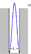
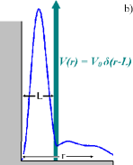
Figure 1: (Color online) Scheme of the Winter model. a) The initial state is the ground state of an infinite square well. b) One of the walls is replaced by a delta barrier $V=V_{0}\delta(r-L)$.

The initial state is an eigenstate of the infinite square well potential,

$$\langle r|\Psi_{0}\rangle=\left\{\begin{array}[]{cl}\sqrt{\frac{2}{L}}\sin\left(\frac{n\pi r}{L}\right)&r\leq L\\ 0&r\geq L\end{array}\right.,$$ (23)

and the $k$-normalized basis functions are

$$\langle r|w_{k}\rangle=e^{-i\delta(k)}\,\sqrt{\frac{2}{\pi}}\,\left\{\begin{array}[]{lr}\sin(kr)/f(k)&r\leq L\\ (i/2)[e^{-ikr}-S(k)e^{ikr}]&r\geq L\end{array}\right.,$$ (24)

where $S(k)=f(k)^{*}/f(k)$, and the Jost function for this model is

$$f(k)=1+\frac{\alpha}{2ik}(e^{2ikL}-1),$$ (25)

with $\alpha=2mV_{0}/\hbar^{2}$. $\rho(v)=|\langle w_{k}|\Psi_{0}\rangle|^{2}m/\hbar$ can be calculated exactly and takes the form

$$\rho(v) = \frac{Lm}{\pi\hbar}\frac{k^{2}}{k^{2}+\alpha k\sin(2kL)+\alpha^{2}\sin^{2}(kL)}$$ (26)

$$\qquad\times\quad\left[\frac{2n\pi\sin(kL)}{k^{2}L^{2}-n^{2}\pi^{2}}\right]^{2}.$$

From here the exact classical probability density is calculated numerically using Eq. (4), whereas the quantum density is given by the square modulus of Eq. (9). In the large-$t$ region the probability density has analytical expressions in both quantum and classical cases given by Eqs. (19) and (21) respectively. The coefficient $\beta$ is easy to find from Eq. (26) in the limit $v\to 0$,

$$\beta=\frac{4m^{3}L^{3}}{(1+\alpha L)^{2}n^{2}\pi^{3}\hbar^{3}}.$$ (27)

Also, Eq. (24) and $S(k)=e^{2i\delta(k)}$, give for the Winter model the explicit source shift

$$a_{0}=\frac{\alpha L^{2}}{1+\alpha L},$$ (28)

which, for $\alpha\geq 0$, lies between $0$ (for $\alpha L\to 0$, no barrier), and $L$ (for large $\alpha L$, strong confinement).

Finally, the quantum and classical probability densities both take (shifting the classical point source by $a_{0}$) the post-exponential form

$$P_{q,c}(r,t)\sim\frac{4}{n^{2}(1+\alpha L)^{2}}\left(\frac{Lm}{\pi\hbar}\right)^{3}\left(r-\frac{\alpha L^{2}}{1+\alpha L}\right)^{2}\frac{1}{t^{3}}.$$ (29)

The agreement is illustrated in Fig. 2, where the exact decay curves (numerically integrated) are plotted. The classical density (triangles) indeed reproduces the quantum behavior (solid line) if the source shift is taken into account. For comparison we also show a curve in which the shift is not applied, so that the classical source remains at $r=0$ (circles). Taking the same value for $\tau$, we see that the classical model also agrees with the quantum one in the pre-exponential and exponential zones ($0<t<5$ in the drawing). The classical model differs only in the absence of oscillations which occur at the onset of post-exponential behavior, due to quantum interference. The asymptotic behavior is indistinguishable on the scale of the figure from the analytical expression Eq. (29).

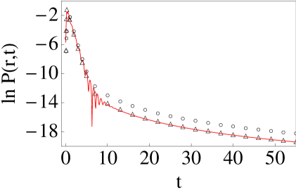
Figure 2: (Color online) The exact probability density obtained numerically versus $t$: quantum result solid (red) line; classical solution including the source shift, Eq. (28)(triangles); classical solution without applying the source shift (circles). Parameter values: $\hbar=1$, $m=1/2$, $L=1$, $\alpha=5$, $n=1$, $r=2$, $\tau=0.5$.

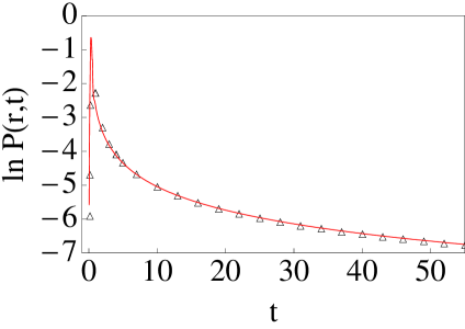
Figure 3: (Color online) Logarithm of the probability density versus $t$, for an attractive delta potential having a zero energy resonance: exact quantum numerical solution (solid red line); classical model solution (triangles). The long-time behaviour is indistinguishable from Eq. (30). $\alpha=-1$, $\tau=0.2$, and other parameters as in Fig. 2.

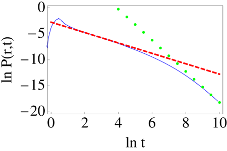
Figure 4: (Color online) Logarithm of the probability density versus $t$ for a delta potential slightly less attractive than required to produce a zero energy resonance: exact quantum numerical solution (solid blue line), and approximate power law decays proportional to $t^{-1}$ (Eq. (30), dashed red line) and $t^{-3}$ (Eq. (29), dotted green line). $\alpha=-0.98$, $r=10$, $\tau=0.2$, and other parameters as in Fig. 2.

The exceptional case of a zero energy resonance corresponds to an attractive delta with $\alpha=-1/L$. In this case from Eqs. (7,22) we get

$$P_{q,c}(x,t)\sim\frac{4Lm}{\hbar n^{2}\pi^{3}t}$$ (30)

for both the classical and quantum cases: see Fig. 3. If $\alpha$ is close to the critical value, say $\alpha=-1/L+\epsilon$, the decay follows a $t^{-1}$ decay law for some substantial period of time until the $t^{-3}$ decay eventually dominates, see Fig. 4. The smaller is $\epsilon$, the longer does the $t^{-1}$ behaviour persist.

IV Discussion

To summarize, the above results provide an intuitive physical picture and quantitative description of post-exponential decay of the probability density at points distant from the source. We have developed the classical model suggested by Newton so as to achieve an accurate match between classical and quantum decays. Purely exponential decay from a source leads naturally, because of dispersion associated with a velocity distribution of the emitted particles, to the same power law decay in quantum and classical scenarios. Quantum mechanics is required to provide the emission characteristics, but initial state reconstruction (ISR) plays no role in the classical, purely outgoing dynamics. We have checked with the methodology of ISR , that ISR-terms are negligible in the post-exponential range of times, in the quantum calculation of Fig. 2. This contrasts with their relevance to the survival probability ISR and indicates different mechanisms for the transition to post-exponential decay inside and outside the source. Indeed, the survival probability (calculated either as $|\langle\Psi(0)|\Psi(t)\rangle|^{2}$ or $|\langle r|\Psi(t)\rangle|^{2}$ with $r<L$ ) is still in its exponential regime when the transition shown in Fig. 2 (at $r=2$) takes place, i.e., the purely exponential decay hypothesis (1) for the classical source is justified, and the onset of the post-exponential regime of survival within the trap cannot causally affect the transition observed in the density outside the source.

Due to recent advances in lasers, semiconductors, nanoscience, and cold atoms, microscopic interactions are now relatively easy to manipulate, decay parameters have become controllable, and post-exponential decay more accessible to experimental scrutiny and/or applications TMMS . Under appropriate conditions it could become the dominant regime and be used to speed-up decay via an Anti-Zeno effect Lewenstein . Moreover, recent experiments on periodic waveguide arrays provide a classical, electric field analog of a quantum system with exponential decay Lon06a ; VLL07 , where the post-exponential region could be studied in a particularly direct way.

References

- (1) L. M. Krauss and J. Dent, Phys. Rev. Lett. 100, 171301 (2008).
- (2) R. G. Winter, Phys. Rev. 126, 1152 (1962).
- (3) C. A. Nicolaides and D. R. Beck, Phys. Rev. Lett. 38, 683, 1037 (1977).
- (4) C. A. Nicolaides, Phys. Rev. A 66, 022118 (2002).
- (5) E. B. Norman, B. Sur, K. T. Lesko, R. M. Larimer, D. J. DePaolo, and T. L. Owens, Phys. Lett. B 357, 521 (1995).
- (6) C. Rothe, S. I. Hintschich, and A. P. Monkman, Phys. Rev. Lett. 96, 163601 (2006).
- (7) J. Martorell, J. G. Muga, and D. W. L. Sprung, in Time in Quantum Mechanics, vol. 2, ed. by J. G. Muga, A. Ruschhaupt, and A. del Campo (Springer, Berlin, 2009).
- (8) E. Torrontegui, J. G. Muga, J. Martorell and D. W. L. Sprung, Phys. Rev. A 80, 012703 (2009).
- (9) R. G. Newton, Ann. Phys. (NY) 14, 333 (1961).
- (10) R. G. Newton, Scattering Theory of Waves and Particles, Second Ed. (Dover, Mineola, 2002).
- (11) L. A. Khalfin, Soviet Physics JETP 6, 1053 (1958).
- (12) J. Petzold, Z. Phys. 155, 422 (1959).
- (13) R. G. Winter, Phys. Rev. 123, 1503 (1961).
- (14) R. Landauer, private conversation with J. G. Muga.
- (15) E. J. Hellund, Phys. Rev. 89, 919 (1953).
- (16) R. Jacob R. G. Sachs, Phys. Rev. 121, 350 (1961).
- (17) C. B. Chiu, E. C. G. Sudarshan, B. Misra, Phys. Rev. D 17, 520 (1977).
- (18) H. M. Nussenzveig, Causality and Dispersion Relations (Academic Press, New York, 1972).
- (19) J. G. Muga, V. Delgado, R. F. Snider, Phys. Rev. B 52, 16381 (1995).
- (20) L. Ersak, Yad. Fiz. 9, 458 (1969); English translation: Sov. J. Nucl. Phys. 9, 263 (1969).
- (21) L. Fonda, G. C. Ghirardi, Il Nuovo Cimento 7A, 180 (1972)
- (22) J. Martorell, J. G. Muga, and D. W. L. Sprung, Phys. Rev. A 77, 042719 (2008).
- (23) J. R. Taylor, Scattering Theory (Wiley, New York, 1972).
- (24) E. T. Whittaker and G. N. Watson, A Course of Modern Analysis (Cambridge, fourth edn. 1927) p. 172.
- (25) J. G. Muga, F. Delgado, A. del Campo, and G. García-Calderón, Phys. Rev. A 73, 052112 (2006).
- (26) M. Lewenstein and K. Rzazewski, Phys. Rev. A 61, 022105 (2000).
- (27) S. Longhi, Phys. Rev. Lett. 97, 110402 (2006).
- (28) G. Della Valle, S. Longhi, P. Laporta, P. Biagioni, L. Dou, and M. Finazzi, Appl. Phys. Lett. 90, 261118 (2007).