Enhancing the spectral gap of networks by node removal

Abstract

Dynamics on networks are often characterized by the second smallest eigenvalue of the Laplacian matrix of the network, which is called the spectral gap. Examples include the threshold coupling strength for synchronization and the relaxation time of a random walk. A large spectral gap is usually associated with high network performance, such as facilitated synchronization and rapid convergence. In this study, we seek to enhance the spectral gap of undirected and unweighted networks by removing nodes because, practically, the removal of nodes often costs less than the addition of nodes, addition of links, and rewiring of links. In particular, we develop a perturbative method to achieve this goal. The proposed method realizes better performance than other heuristic methods on various model and real networks. The spectral gap increases as we remove up to half the nodes in most of these networks.

I Introduction

Various systems of interacting elements can be represented by networks that consist of a set of nodes and links that connect pairs of nodes. The structure of networks affects various dynamics occurring on the networks Pikovsky01book ; Boccaletti06PR ; Barrat08book .In particular, many dynamics on networks are controlled by a few extremal eigenvalues of the adjacency matrix and the Laplacian matrix of the network (see Sec. II for the definition of the Laplacian matrix). The values of these eigenvalues provide concise and useful information about the dynamics on the networks.

In this study, we focus on the second smallest eigenvalue of the Laplacian matrix; it is called the spectral gap and is denoted by $\lambda_{2}$ in this paper. We examine $\lambda_{2}$ because it characterizes a wide class of dynamics on networks as follows. First, a network with a large value of $\lambda_{2}$ decreases the threshold of coupling strength for synchronization for both linear dynamics and some nonlinear dynamics including coupled oscillators on networks Pikovsky01book ; Boccaletti06PR ; Barrat08book ; Almendral07new ; Arenas08pr ; Motter07new ; Donetti06jstatm . Such a family of nonlinear dynamics is called the class II Boccaletti06PR ; Almendral09pre or type II Arenas08pr dynamics. Note that the largest Laplacian eigenvalue as well as $\lambda_{2}$ is an important determinant of the synchronizability in the so-called class III Boccaletti06PR ; Almendral09pre or type I Arenas08pr dynamics. However, we are not concerned with class III or type I dynamics in this paper. Second, when $\lambda_{2}$ is large, synchronization in these dynamics Almendral07new and consensus dynamics Olfati07 occur rapidly in certain types of networks. Third, $\lambda_{2}$ characterizes the convergence speed of the Markov chain on the network to the stationary density Donetti06jstatm ; Cvetkovic10book . Fourth, the first-passage time of the random walk is characterized by $\lambda_{2}$ Donetti06jstatm . Fifth, the duality between the coalescing random walk and the voter model Liggett85book-Durrett88book implies that $\lambda_{2}$ also determines the consensus time of the stochastic voter dynamics. This is in agreement with the results obtained for the majority-vote spin dynamics on networks Almendral07new . In addition to these dynamical properties of networks, various graph-theoretical structural properties of networks are characterized by $\lambda_{2}$ Mohar91book ; Cvetkovic10book .

In these applications, a large value of $\lambda_{2}$ is usually preferred because it indicates, for example, enhanced synchronizability and fast convergence. Consequently, the enhancement of $\lambda_{2}$ has been explored in the framework of designing of networks Motter07new ; Nishikawa06PRE_PhyD and numerical optimization via the rewiring of links Donetti05prl ; Donetti06jstatm . In practice, however, rewiring links, constructing optimized networks from scratch, and adding nodes or links are likely to cost more than the removal of nodes or links of a given network. The effects of removal of nodes or links have been investigated in the context of the cascading failure Motter04prl and the influence on extreme eigenvalues of the adjacency matrix Restrepo06prl . With regard to Laplacian eigenvalues, the removal of links always decreases $\lambda_{2}$ and makes the network less likely to synchronize Milanese10pre ; Nishikawa2010PNAS . However, to the best of our knowledge, whether or not careful removal of nodes may increase $\lambda_{2}$ has not yet been examined. We treat this problem in the present paper.

Although removal of nodes generally decreases the magnitude of activities, stabilizing synchronization at the expense of the magnitude is valuable in some applications. The treatment of cardiac arrhythmia is one of the examples. The heart consists of a large number of cardiac cells that show nonlinear dynamics Guevara1981Science_Chialvo1987Nature . Synchronized dynamics of cardiac cells create physiological heart beats Bub1998PNAS_GuytonBook . Cardiac arrhythmia is considered to be caused by malfunction of synchronization. The catheter ablation aims at restoring synchrony of the entire heart by electrically deactivating some cardiac cells that prevent synchronization Glass01nat . As another example, proper operations of power plant networks also critically require that the frequency of voltage among power plants is synchronized Filatrella2008EPJ ; Fioriti2009CIIS . Loss of the synchronization may induce a blackout in the entire network. Therefore, it is likely that stable synchrony at the expense of some total power supply serves steady supplying of electricity to the entire network Filatrella2008EPJ .

We compare various strategies for maximizing $\lambda_{2}$ by sequential node removal on various model and real networks. In particular, we develop a perturbative strategy that is applicable to relatively large networks in terms of the computational cost. We show that the performance of the perturbative strategy is comparable to that of the computationally costly optimal sequential strategy and is generally better than that of heuristic strategies. In addition, in many examined examples, $\lambda_{2}$ continues to increase until we remove a fairly large fraction of nodes ($\approx$ 50%) sequentially according to the perturbative strategy.

II Strategies for sequential node removal

We consider undirected and unweighted connected networks with $N$ nodes. The Laplacian matrix $L$ is defined as follows. $L_{ij}$ ($1\leq i\neq j\leq N$) is equal to $-1$ if node $i$ and $j$ are connected and 0 otherwise; $L$ is a symmetric matrix. The diagonal is given by $L_{ii}=k_{i}$, where $k_{i}$ is the degree of node $i$. Note that $\sum_{j=1}^{N}L_{ij}=0$ for each $i$. $L$ has $N$ (real) nonnegative eigenvalues $0=\lambda_{1}<\lambda_{2}\leq\cdots\leq\lambda_{N}$. We seek to maximize $\lambda_{2}$ upon sequential removal of nodes. We compare the effectiveness of the following node removal strategies by applying them to model and real networks.

• Degree-based strategy: In each step, we remove the node with the smallest degree in the remaining network. The rationale behind this strategy is that the smallest degree controls $\lambda_{2}$, with a useful bound being $\lambda_{2}\leq k_{\min}N/(N-1)$, where $k_{\min}$ is the smallest degree in the network Arenas08pr ; Mohar91book ; Cvetkovic10book . If there exist multiple nodes having the same smallest degree, we select one of them with an equal probability.

  In intentional attacks on networks, where the aim is to fragment the network into disjoint components with a small number of removed nodes, removing nodes with the largest degree is an effective strategy Albert00nat-Callaway00prl-Cohen01prl . We implemented this strategy but obtained poor results for our purpose, and therefore we do not mention it in the following.

• Betweenness-based strategy: In each step, we remove the node with the smallest betweenness centrality. The betweenness centrality of node $i$ is defined as follows. Denote by $\sigma_{i_{1}i_{2}}$ the number of the shortest paths between nodes $i_{1}$ and $i_{2}$, and by $\sigma_{i_{1}i_{2}}(i)$ the number of the shortest paths between them that pass through node $i$. We set $\sigma_{i_{1}i_{2}}(i_{1})=\sigma_{i_{1}i_{2}}(i_{2})=0$. The betweenness centrality of node $i$ is proportional to $\sum_{i_{1}=1;i_{1}\neq i}^{N}\sum_{i_{2}=i_{1}+1;i_{2}\neq i}^{N}\sigma_{i_{1}i_{2}}(i)/\sigma_{i_{1}i_{2}}$ Freeman79 ; Boccaletti06PR ; Barrat08book . Sequentially removing nodes with the largest betweenness centrality yielded poor results, and therefore we do not mention it in the following.

• Optimal sequential strategy: We calculate the change in $\lambda_{2}$ induced by the removal of each node by direct numerical simulations. Then, we select the node whose removal increases $\lambda_{2}$ by the largest amount. Note that this strategy is computationally costly because it requires the calculation of $\lambda_{2}$ for $N$ different networks, each having $N-1$ nodes. Calculating $\lambda_{2}$ for a single network requires $\mathrm{O}(N^{3})$ time. Therefore, carrying out a single step of the optimal sequential strategy requires $\mathrm{O}(N^{4})$ time.

• Perturbative strategy: To avoid the computational cost of the optimal sequential strategy, we develop an approximate perturbative strategy defined as follows. Related perturbative calculations are treated in Restrepo06prl ; Masuda09njp ; Milanese10pre .

  Let us represent the eigen equation for $\lambda_{2}$ as $L\bm{u}=\lambda_{2}\bm{u}$, where $\bm{u}$ is the $N$-dimensional eigenvector of $L$ corresponding to $\lambda_{2}$. The eigenvector $\bm{u}$ is normalized such that $\sum_{i=1}^{N}u_{i}^{2}=1$, where $u_{i}$ is the $i$th element of $\bm{u}$. The eigen equation after the removal of node $i$ is given by

  $$(L+\Delta L)(\bm{u}+\Delta\bm{u})=(\lambda_{2}+\Delta\lambda_{2})(\bm{u}+\Delta\bm{u}),$$ (1)

  where the changes in $L$, $\lambda_{2}$, and $\bm{u}$ induced by the removal of node $i$ are denoted by $\Delta L$, $\Delta\lambda_{2}$, and $\Delta\bm{u}$, respectively. Because $L$ is symmetric, the displacement matrix $\Delta L$ is given by $(\Delta L)_{ii}=-L_{ii}=-k_{i}$, $(\Delta L)_{jj}=L_{ji}(j\neq i)$, and $(\Delta L)_{ji}=(\Delta L)_{ij}=-L_{ji}(j\neq i)$. Because the $i$th component of $\bm{u}+\Delta\bm{u}$ is equal to zero, we write $\Delta\bm{u}=\delta\bm{u}-u_{i}\hat{\bm{e}}_{i}$, where $\hat{e_{i}}$ is the unit vector for the $i$th component and $\delta\bm{u}$ is an $N$-dimensional vector. By multiplying the normalized left eigenvalue $\bm{u}^{\top}$ ($\top$ denotes the transpose) from the left of Eq. (1), we obtain

  $$\Delta\lambda_{2}=\frac{\bm{u}^{\top}\Delta L(\bm{u}-u_{i}\hat{\bm{e}}_{i}+\delta\bm{u})}{\bm{u}^{\top}(\bm{u}-u_{i}\hat{\bm{e}}_{i}+\delta\bm{u})}$$ (2)

  We assume that the absolute value of each element of $\delta\bm{u}$ is smaller than that of $\bm{u}-u_{i}\hat{\bm{e}}_{i}$. Then, by ignoring $\delta\bm{u}$ in Eq. (2) and substituting the expression for $\Delta L$ in Eq. (2), we obtain

  $$\Delta\lambda_{2}\approx\frac{\sum_{j\in{\mathcal{N}}_{i}}u_{j}(u_{i}-u_{j})}{1-u_{i}^{2}},$$ (3)

  where ${\mathcal{N}}_{i}$ indicates the neighborhood of node $i$.

  In the perturbative strategy, we remove node $i$ that maximizes $\Delta\lambda_{2}$ given by Eq. (3). Note that carrying out one step of the perturbative strategy requires solving the eigen equation just once. Therefore, the computation cost is $\mathrm{O}(N^{3})$, which is $N$ times smaller than that for the optimal sequential strategy. In the following numerical simulations, the networks are connected during sequential node removal for all the networks and strategies.

III Results

In this section, we apply the node-removal strategies introduced in Sec. II to various model and real networks.

III.1 Model networks

First, we apply different strategies to the following types of model networks.

• Erdős-Rényi (ER) random graph with mean degree $\left<k\right>=p(N-1)$, where $p$ is the probability that a link exists between a pair of nodes.

• Watts-Strogatz (WS) model Watts98nat , where each node is connected to $\left<k\right>/2$ closest nodes on each side along the ring and a fraction, 0.3, of links are rewired randomly.

• Barabási-Albert (BA) model Barabasi99sci , a representative growing scale-free network model. We start the growth of the network from the complete graph of $m$ nodes and add a node with $m$ links one-by-one according to the preferential attachment. We obtain $\left<k\right>\approx 2m$, degree distribution $p(k)\propto k^{-3}$, and low clustering.

• Holme-Kim (HK) model Holme02pre , a growing scale-free network model. The algorithm of the HK model is similar to that of the BA model. The difference is that, when a node is added, the preferential attachment is used with a certain probability, which we set as 0.5. With the remaining probability (i.e., 0.5), we use the so-called triad formulation rule to enhance clustering. We obtain $\left<k\right>\approx 2m$, degree distribution $p(k)\propto k^{-3}$, and high clustering.

• Goh model Goh01prl , a nongrowing scale-free network model. We assign the weight $w_{i}=i^{-0.5}$ to each node $i$. Then, we select a pair of nodes with the probability proportional to $w_{i}$ and connect them. We repeat this procedure until we obtain the desired mean degree $\left<k\right>$. We obtain $p(k)\propto k^{-3}$.

For each network model, we assume two values of $\left<k\right>$. For each case, we carry out sequential node removal according to different strategies. Because, in stepwise node removal, the optimal sequential strategy is usually an efficient way, we will mainly evaluate the effectiveness of the other strategies using the performance of the optimal sequential strategy as a baseline.

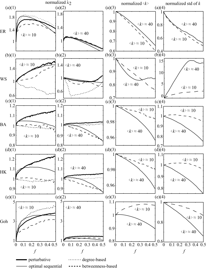
Figure 1: Numerical results for model networks with $N=250$ nodes. We set $\left<k\right>=10$ and $\left<k\right>=40$ for each network. (a) ER random graph, (b) WS model, (c) BA model, (d) HK model, and (e) Goh model. (a)(1), (a)(2), (b)(1), (b)(2), (c)(1), (c)(2), (d)(1), (d)(2), (e)(1), and (e)(2) show the change in $\lambda_{2}$ induced by each strategy. The mean degrees are shown in the panels. (a)(3), (b)(3), (c)(3), (d)(3), and (e)(3) show the change in the mean degree with node removal. (a)(4), (b)(4), (c)(4), (d)(4), and (e)(4) show the change in the standard deviation of the degree with node removal.

The numerical results obtained for the networks with $N=250$ averaged over 10 trials are shown in Fig. 1. Figures 1(a)(1) and 1(a)(2) show the values of $\lambda_{2}$ after removing a fraction of nodes for two ER random graphs with different values of $\left<k\right>$. The fraction of the removed nodes is denoted by $f$. For each strategy, $\lambda_{2}$ increases slightly in the early stages (i.e., $0<f<0.05$). Then, $\lambda_{2}$ starts to decrease even for the optimal sequential and perturbative strategies, which are designed to maximize $\lambda_{2}$. Surprisingly, in the network with larger $\left<k\right>$ (Fig. 1(a)(2)), the optimal sequential strategy is not as efficient as the other strategies as $f$ increases. This is possible because the optimal sequential strategy finds the stepwise best strategy and does not take into account the performance after multiple nodes are removed. The perturbative strategy remains more efficient or as efficient as the optimal sequential strategy when $f$ is large.

For the WS model with different mean degrees (Fig. 1(b)(1) and 1(b)(2)), the optimal sequential and perturbative strategies outperform the heuristic degree-based and betweenness-based strategies. As in the case of the ER random graph, the perturbative strategy is as efficient as the optimal sequential strategy.

The performances of the perturbative strategies are also good among the competitive strategies for different scale-free network models (Fig. 1(c)(1), 1(c)(2), 1(d)(1), and 1(d)(2)). In Goh model(Fig. 1(e)(1) and 1(e)(2)), thought it is not better than the degree-based strategy, the perturbative strategy is better than the optimal sequential strategy except for in the early stage (i.e. $0<f<0.3$) in the Goh model with the smaller degree (Fig. 1(e)(1)). Note that for the three scale-free network models, $\lambda_{2}$ continues to increase even until half the nodes are removed.

Changes in $\left<k\right>$ and the standard deviation of the degree with node removal according to the perturbative strategy are shown in Fig. 1(a)(3), 1(a)(4), 1(b)(3), 1(b)(4), 1(c)(3), 1(c)(4), 1(d)(3), 1(d)(4), 1(e)(3), and 1(e)(4). The direction of changes in $\left<k\right>$ and that of the standard deviation of the degree depend on the network model. For example, in the Goh model, nodes with small degree are preferentially removed in general, especially for small $f$ (Fig. 1(e)(3)). However, the removed nodes are not generally those with the smallest degrees; the degree-based strategy performs relatively poorly (Fig. 1(b)(1), 1(b)(2), 1(c)(1), 1(c)(2), 1(d)(1), 1(d)(2), 1(e)(1), and 1(e)(2)). In contrast, in the ER, WS, BA, and HK models, the perturbative strategy removes nodes with appropriately large degree (Fig. 1(a)(3), 1(b)(3), 1(c)(3), and 1(d)(3)). Similarly, the perturbative strategy increases $\lambda_{2}$ by increasing the heterogeneity of degree in the WS model (Fig. 1(b)(4)) and by decreasing the same heterogeneity in the other four network models (Fig. 1(a)(4), 1(c)(4), 1(d)(4), and 1(e)(4)). These show that the perturbative strategy adapts itself for each network.

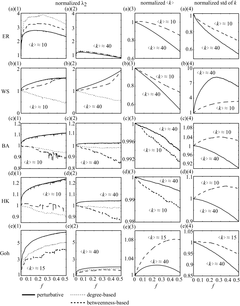
Figure 2: Numerical results for (a) ER model, (b) WS model, (c) BA model, (d) HK model, and (e) Goh model with $N=2000$. We set $\left<k\right>=10$ and $\left<k\right>=40$ for each network model with one exception. We use $\left<k\right>=15$ instead of $\left<k\right>=10$ for the Goh model because the Goh model with $N=2000$, $\left<k\right>=10$, and $w_{i}=i^{-0.5}$ ($1\leq i\leq N$) rarely yields a connected network.

Next, we compare the efficiency of different strategies on larger networks ($N=2000$). We exclude the optimal sequential strategy because the large $N$ hinders its implementation. In this set of numerical simulations, we are mainly concerned with the performance of the perturbative strategy. The numerical results obtained on the basis of 5 realizations of each network are shown in Fig. 2. These results are qualitatively the same as those obtained for the smaller networks shown in Fig. 1. The perturbative strategy enhances $\lambda_{2}$ more efficiently than the other heuristic strategies except in ER models. In addition, the behavior of the perturbative strategy cannot be simply captured by the changes in $\left<k\right>$ or the standard deviation of the degree, which is again qualitatively the same as the results shown in Fig. 1.

III.2 Real networks

We apply the proposed strategies to the largest connected component of the following real networks: the C. elegans neural network Chen06pnas ; wormatlas , E. coli metabolic network Jeong00nat , e-mail social network Guimera03pre , and macaque cortical network Felleman91cc-Young93pbs-SpornsZwi04ni . We ignore the direction of links in the C. elegans neural network and the macaque cortical network, both of which are originally directed networks. In the C. elegans neural network, two neurons are regarded to be connected when they are connected by at least one chemical synapse or gap junction.

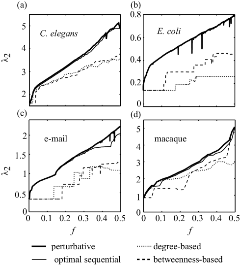
Figure 3: Numerical results for real networks. (a) C. elegans neural network with $N=279$ and $\left<k\right>=16.4$. (b) E. coli metabolic network with $N=2268$ and $\left<k\right>=4.96$. (c) E-mail social network with $N=1133$ and $\left<k\right>=9.62$. (d) Macaque cortical network with $N=71$ and $\left<k\right>=12.3$.

The efficiency of different strategies on these real networks is shown in Fig. 3. The perturbative strategy enhances $\lambda_{2}$ more efficiently in all the tested real networks than the degree-based and betweenness-based strategies. Except in the case of the E. coli metabolic network, which is too large for the optimal sequential strategy, the results for the optimal sequential strategy are shown as well (Fig. 3(a), 3(c), and 3(d)). The perturbative strategy performs roughly as well as the optimal sequential strategy in these networks.

III.3 Comparison to the rewiring strategy

One can alternatively enhance $\lambda_{2}$ by rewiring links Donetti05prl ; Donetti06jstatm . In the rewiring strategy, we sequentially rewire links to increase $\lambda_{2}$. In each step, we examine the increase in $\lambda_{2}$ for all the possible patterns of single-link rewiring and adopt the one that increases $\lambda_{2}$ by the largest amount. To compare the performance of the node removal and the rewiring, we carry out numerical simulations using the ER and BA models with $N=50$ and $\left<k\right>=4$. We simulate the rewiring process just once for each network because the rewiring strategy is computationally costly.

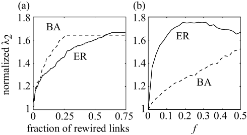
Figure 4: Numerical results for the ER and BA models with $N=50$. (a) Results for link rewiring. The normalized $\lambda_{2}$ is plotted against the number of rewired links. (b) Results for node removal. The normalized $\lambda_{2}$ averaged over 10 realizations is plotted against the number of removed nodes. We set $\left<k\right>=4$ in both networks.

The change in $\lambda_{2}$ relative to the initial value during the rewiring process is shown in Fig. 4(a). $\lambda_{2}$ is enhanced up to about 1.7 fold for both networks. The corresponding results for the sequential node removal according to the perturbative strategy are shown in Fig. 4(b). Roughly speaking, the performance of the perturbative strategy is comparable to that of the rewiring strategy. The perturbative strategy is superior to the rewiring strategy for the ER model and vice versa for the BA model. Because the rewiring strategy is computationally costly and may be too demanding to be implemented in some real applications, the node removal according to the perturbative strategy seems to be a feasible choice for enhancing $\lambda_{2}$.

III.4 Accuracy of the perturbative strategy

When deriving the perturbative strategy, we crucially assumed that $\delta\bm{u}$ is negligible as compared to $\bm{u}-u_{i}\hat{\bm{e}}_{i}$. We justify this assumption as follows. A node that is removed according to the perturbative strategy tends to have large $\Delta\lambda_{2}$ and a small degree. If the removed node has a small degree, the number of the nonzero entries of the corresponding $\Delta L$ is relatively small. Therefore, a relatively small number of the entries of $\bm{u}$ would be directly affected by the node removal, and we would obtain a small $\delta\bm{u}$.

To probe the validity of this assumption and quantify the error in estimating $\Delta\lambda_{2}$, we measure two kinds of relative estimation error during the course of sequential node removal according to the perturbative strategy. The first quantity is the average of $|(\delta\bm{u})_{j}/(\bm{u}-u_{i}\hat{\bm{e}}_{i})_{j}|$ over node $j$ ($1\leq j\leq N$, $j\neq i$), where $i$ is the index of the removed node. The second quantity is the difference between $\Delta\lambda_{2}$ obtained from the perturbative strategy and the actual $\Delta\lambda_{2}$, which is normalized by the actual $\Delta\lambda_{2}$. We take averages of these quantities over 200 generated networks having $N=250$.

For the five network models, $|(\delta\bm{u})_{j}/(\bm{u}-u_{i}\hat{\bm{e}}_{i})_{j}|$ for $\left<k\right>=10$ and $\left<k\right>=40$ is shown in Fig. 5(a) and 5(b), respectively. The magnitude of $\delta\bm{u}$ relative to that of $\bm{u}-u_{i}\hat{\bm{e}}_{i}$ is sufficiently small. The relative estimation error in $\Delta\lambda_{2}$ for the removed nodes is shown for $\left<k\right>=10$ and $\left<k\right>=40$ in Fig. 5(c) and 5(d), respectively. As expected, the relative estimation error in $\Delta\lambda_{2}$ is generally small. We conclude that, up to our numerical efforts, the perturbative strategy does not suffer from a crucially large error.

IV Conclusions

We explored efficient strategies to sequentially remove nodes of networks in order to increase or maintain a large value of the spectral gap (i.e., second smallest eigenvalue of the Laplacian matrix) of the undirected and unweighted network. We introduced a perturbative strategy among others. For a variety of networks, this strategy generally performed well as compared to heuristic strategies in which we sequentially remove the nodes with the smallest degree or the smallest betweenness centrality. In most of our numerical results, the spectral gap increased until the removal of a fairly large fraction of nodes ($\approx$ 50%). Occasionally, the perturbative strategy is even more efficient than the optimal sequential strategy, despite its decreased computational cost. Although we focused on unweighted networks, the extension of the perturbative strategy to the case of weighted networks is straightforward.

In chaotic dynamical systems on networks, synchronization is often facilitated by a small value of $R=\lambda_{N}/\lambda_{2}$, where $\lambda_{2}$ and $\lambda_{N}$ are the second smallest eigenvalue and the largest eigenvalue of the Laplacian matrix, respectively. Dynamics whose synchronizability is determined by $R$ belongs to the class III Boccaletti06PR ; Almendral09pre (also termed type I Arenas08pr ). In contrast, we have been concerned with the synchronization of the class II Boccaletti06PR ; Almendral09pre (also termed type II Arenas08pr ) dynamics in which synchronization is facilitated in networks with large $\lambda_{2}$. To address class III or type I synchronizability, we developed the perturbative strategy for minimizing $R$ upon the removal of nodes and assessed its efficiency on some model networks. However, the results were generally poor (results not shown). The perturbative strategy failed mainly because it does not accurately estimate the change in $\lambda_{N}$. The applicability of our results is limited to class II or type II dynamics.

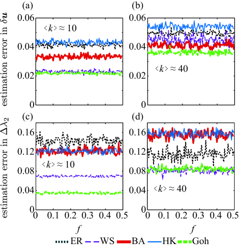
Figure 5: (Color online) Relative estimation error in (a, b) $\delta\bm{u}$ and (c, d) $\Delta\lambda_{2}$. See Sec. III.4 for the definitions of the relative estimation error. We set (a, c) $\left<k\right>=10$ and (b, d) $\left<k\right>=40$. We use $\left<k\right>=15$ instead of $\left<k\right>=10$ for the Goh model because the Goh model with $N=250$, $\left<k\right>=10$, and $w_{i}=i^{-0.5}$ ($1\leq i\leq N$) rarely yields a connected network.

- (1) A. Pikovsky, M. Rosenblum, and J. Kurths, Synchronization – A Universal Concept in Nonlinear Sciences (Cambridge University Press, Cambridge, UK, 2001).
- (2) S. Boccaletti, V. Latora, Y. Moreno, M. Chavez, and D.-U. Hwang. Phys Rep 424, 175(2006) .
- (3) A. Barrat, M. Barthélemy, and A. Vespignani, Dynamical Processes on Complex Networks, (Cambridge University Press, Cambridge, UK, 2008).
- (4) A. Arenas, A. Diaz-Guilera, J. Kurths, Y. Moreno, and C. Zhou, Phys. Rep. 469, 93 (2008).
- (5) J.A. Almendral and A. Diaz-Guilera, New J. Phys. 9, 187 (2007).
- (6) A. E. Motter, New J. Phys., 9, 182 (2007).
- (7) T. Nishikawa and A. E. Motter. Phys. Rev. E 73, 065106 (2006); T. Nishikawa and A. E. Motter. Physica D 224, 77 (2006).
- (8) L. Donetti, F. Neri, and M.A. Muñoz, J. Stat. Mech.: Theory Exp. (2006). P08007.
- (9) J. A. Almendral, I. Sendiña-Nadal, D. Yu, I. Leyva, and S. Boccaletti. Phys. Rev. E 80 066111 2009
- (10) R. Olfati-Saber, J.A. Fax, and R. M. Murray, Proc. IEEE 95, 215 (2007).
- (11) D. Cvetković, P. Rowlinson, and S. Simić, An Introduction to the Theory of Graph Spectra (Cambridge University Press, Cambridge, UK, 2010).
- (12) T.M. Liggett, Interacting Particle Systems (Springer, New York, 1985); D. Durrett, Lecture Notes on Particle Systems and Percolation (Wadsworth, Belmont, 1988).
- (13) B. Mohar, The Laplacian Spectrum of Graphs, in Y. Alavi, G. Chartrand, O. R. Oellermann, and A. J. Schwenk (Eds.). Graph Theory, Combinatorics, and Applications - Proceedings of the Sixth Quadrennial International Conference on the Theory and Applications of Graphs 2, 871-898 (John Wiley & Sons, Inc., New York, 1991).
- (14) L. Donetti, P.I. Hurtado, and M.A. Muñoz, Phys. Rev. Lett. 95, 188701 (2005).
- (15) A. E. Motter, Phys. Rev. Lett. 93, 098701 (2004).
- (16) J. G. Restrepo, E. Ott, and B. R. Hunt, Phys. Rev. Lett. 97, 094102 (2006).
- (17) A. Milanese, J. Sun, and T. Nishikawa, Phys. Rev. E 81 046112 (2010).
- (18) T. Nishikawa and A. E. Motter. Proc Natl Acad Sci USA 107, 10342 (2010).
- (19) M. R. Guevara, L. Glass, and A. Shrieret. Science 214 1350 (1981); D. R. Chialvo and J. Jalife Nature 330 749 (1987)
- (20) G. Bub, L. Glass, N. G. Publicover, and A. Shrier. Proc Natl Acad Sci USA 95, 10283 (1998); A. C. Guyton and J.E. Hall. Textbook of Medical Physiology (Elsevier Saunder, Philadelphia, 2006)
- (21) L. Glass, Nature 410, 277 (2001).
- (22) G. Filatrella, A. H Nielsen, and N. F. Pedersen Eur Phys J B 61, 485 (2008)
- (23) V. Fioriti, S. Ruzzante, E. Castorini, E. Marchei, and V. Rosato, Critical Information Infrastructure Security, edited by R. Setola and S. Gerestshuber (Springer, New York, 2009), pp. 14-23.
- (24) R. Albert, H. Jeong, and A.L. Barabási, Nature 406, 378 (2000); D.S. Callaway, M.E.J. Newman, S.H. Strogatz, and D.J. Watts, Phys. Rev. Lett. 85, 5468 (2000); R. Cohen, K. Erez, D. ben-Avraham, and S. Havlin, ibid. 85, 4626 (2000).
- (25) L.C. Freeman, Soc. Netw. 1, 215 (1979).
- (26) N. Masuda, New J. Phys. 11, 123018 (2009).
- (27) D.J. Watts and S.H. Strogatz, Nature 393, 440 (1998).
- (28) A.L. Barabási and R. Albert, Science 286, 5439 (1999).
- (29) P. Holme and B.J. Kim, Phys. Rev. E 65, 026107 (2002).
- (30) K.I. Goh, B. Kahng, and D. Kim, Phys. Rev. Lett. 87, 278701 (2001).
- (31) B.L. Chen, D.H. Hall, and D.B. Chklovskii, Proc. Natl. Acad. Sci. USA 103, 4723 (2006).
- (32) http://www.wormatlas.org
- (33) H. Jeong, B. Tombor, R. Albert, Z.N. Oltvai, and A.L. Barabási, Nature 407, 6804 (2000).
- (34) R. Guimerà, L. Danon, A. Diaz-Guilera, F. Giralt, and A. Arenas, Phys. Rev. E 68, 065103(R) (2003).
- (35) D.J. Felleman and D.C. Van Essen, Cereb. Cortex 1, 1 (1991); M.P. Young, Proc. Biol. Sci. London, Ser. B. 252, 13 (1993); O. Sporns and J.D. Zwi, Neuroinformatics 4, 145 (2004).