020002 2010 D. A. Stariolo 020002

A simple Lennard–Jones fluid confined in a slit nanopore with hard walls is studied on the basis of a multilayer structured model. Each layer is homogeneous and parallel to the walls of the pore. The Helmholtz energy of this system is constructed following van der Waals-like approximations, with the advantage that the model geometry permits to obtain analytical expressions for the integrals involved. Being the multilayer system in thermodynamic equilibrium, a system of non-linear equations is obtained for the densities and widths of the layers. A numerical solution of the equations gives the density profile and the longitudinal pressures. The results are compared with Monte Carlo simulations and with experimental data for Nitrogen, showing very good agreement.

Multilayer approximation for a confined fluid in a slit pore

99 inst1 IFLYSIB-Instituto de Física de Líquidos y Sistemas Biológicos (CONICET, UNLP, CICPBA), 59 No. 789, 1900 La Plata, Argentina. inst2 CICPBA-Comisión de Investigaciones Científicas de la Prov. de Buenos Aires.

1 Introduction

The effects on phase transition of confined fluids in a slit-like pore have been studied by simulation and different theories [1–11]. In a previous work, we constructed a generalized van der Waals equation for a fluid confined in a nanopore [12, 13]. The shift of the critical parameters was in good agreement with lattice model and numerical simulation results, and the predicted critical temperature remarkably reproduced the experiment. In that work, we concluded that the confined van der Waals fluid theory seemed to work better than the bulk one, maybe due to the fact that the higher virial contributions not considered in both theories were less important in the confined fluid than in the bulk. A similar treatment was used previously by Schoen and Diestler [14]. Following that line of reasoning, here we study a simple fluid confined between two infinite parallel hard walls (slit pore). The walls are at a distance $\mathit{L}$ apart. To study the confined fluid, we propose a multilayer model [15]: the fluid is distributed in n thin layers, one beside the other. Each layer has a uniform density, and can be observed as a non-autonomous phase. A particle in a given layer interacts with its neighbors inside the layer, and with every particle in the other layers. Defay and Prigogine and Murakami et al. have shown that, in a liquid gas interface, the deviation from the Gibbs’ adsorption equation becomes practically negligible in the case of a two layer model [16], and that as the number of transition layers grows, the multilayer model becomes perfectly consistent with the Gibbs’ equation [17]. The van der Waals-like approximations made in developing this multilayer model theory limit its validity to the low density regime.

2 Theory

The model system consists of a fluid of $\mathit{N}$ Lennard–Jones particles confined in a slit nanopore. The hard walls of the pore, separated at a distance $\mathit{L}$ (in the $\mathit{x}$ direction), have a surface area $\mathit{S}$ ($\mathit{S}\rightarrow\infty$). We divided the fluid into $\mathit{n}$ layers, each layer being parallel to the pore walls. The layer $\mathit{i}$  has $\mathit{N}_{\mathit{i}}$ particles ($\mathit{N}=\sum_{i=1}^{n}N_{i}$), a width $\mathit{L}_{\mathit{xi}}$ ($\mathit{L}$= $\sum_{i=1}^{n}L_{xi}$), and a volume $V_{i}=SL_{xi}$. Then the Helmholtz energy [18] can be written as

$$A=-kT\ln\left(\frac{Z_{N}\lambda^{-3N}}{\prod\limits_{i=1}^{n}N_{i}!}\right).$$ (1)

The configuration integral $\mathit{Z}_{\mathit{N}}$ for a pair potential $\mathit{v}_{\mathit{ij}}$ may be approximated as

$$Z_{N} = \int\prod\limits_{\begin{subarray}{c}i=1\\ i<j\end{subarray}}^{n}e^{-v_{ij}/kT}\mathrm{d}\mathbf{r}^{N}\approx\sum_{\begin{subarray}{c}i=1\\ i<j\end{subarray}}^{n}\int f_{ij}\mathrm{d}\mathbf{r}^{N}$$

$$+\prod\limits_{i=1}^{n}V_{i}^{N_{i}}$$

$$f_{ij} = e^{-v_{ij}/kT}-1,$$

and further expanded in function of two particle integrals

$${Z_{N}} {=} {\sum\limits_{i=1}^{n}\frac{N_{i}(N_{i}-1)}{2}V_{i}^{N_{i}-2}}$$

$${\prod\limits_{\begin{subarray}{c}k=1\\ k\neq i\end{subarray}}^{n}V_{k}^{N_{k}}\int\limits_{R_{i}}f_{12}\mathrm{d}}\mathbf{r}{{}_{\mathbf{1}}\mathrm{d}\mathbf{r}_{\mathbf{2}}}$$

$$+{\sum\limits_{i=1}^{n}\sum\limits_{\begin{subarray}{c}j=2\\ j>i\end{subarray}}^{n}N_{i}N_{j}V_{i}^{N_{i}-1}V_{j}^{N_{j}-1}}$$

$${\prod\limits_{\begin{subarray}{c}k=1\\ k\neq i,k\neq j\end{subarray}}^{n}V_{k}^{N_{k}}\int\limits_{R_{i}}\int\limits_{R_{j}}f_{12}\mathrm{d}}\mathbf{r}{{}_{\mathbf{1}}\mathrm{d}}\mathbf{r}{{}_{\mathbf{2}}+\prod\limits_{i=1}^{n}V_{i}^{N_{i}}}.$$

The first term in Eq. (2) stands for particles in the layer $\mathit{i}$. The second term comes from the interaction of one particle in layer $\mathit{i}$ with one particle in layer $\mathit{j}$. In a compact form, and assuming that a layer sees three nearest neighbor layers,

$$Z_{N} = (\sum\limits_{i=1}^{n}\frac{N_{i}^{2}}{2V_{i}^{2}}I_{i}$$

$$+\sum\limits_{i=1}^{n-1}\sum\limits_{\begin{subarray}{c}j=i+1\\ j\leq n\end{subarray}}^{i+3}\frac{N_{i}}{V_{i}}\frac{N_{j}}{V_{j}}I_{i\,j}+1\,)\prod\limits_{i=1}^{n}V_{i}{}^{N_{i}}.$$

The integrals $\mathit{I}_{\mathit{i}}$ and $\mathit{I}_{\mathit{ij}}$, for the slit pore geometry and after low density approximations, can be analytically solved to give

$$\begin{array}[]{l}{I_{i}=\iint\limits_{R_{i}}f_{12}\mathrm{d}\mathbf{r}_{1}\mathrm{d}\mathbf{r}_{2}\approx-\iint\limits_{\left|\mathbf{r}_{1}\mathrm{-}\mathbf{r}_{2}\right|<\sigma}\mathrm{d}\mathbf{r}_{1}\mathrm{d}\mathbf{r}_{2}}\\ {-\iint\limits_{\left|\mathbf{r}_{1}\mathrm{-}\mathbf{r}_{2}\right|\geq\sigma}\frac{v_{12}}{kT}\mathrm{d}\mathbf{r}_{1}\mathrm{d}\mathbf{r}_{2}=-2V_{i}\sigma^{3}(b-B_{i})-\frac{2V_{i}\sigma^{3}\varepsilon}{kT}A_{i}}\end{array}$$ (5)

$$\begin{array}[]{l}{I_{i,\,i+1}=\int\limits_{R_{i}}\int\limits_{R_{i+1}}f_{12}\mathrm{d}\mathbf{r}_{1}\mathrm{d}\mathbf{r}_{2}\approx-\iint\limits_{\left|\mathbf{r}_{1}\mathrm{-}\mathbf{r}_{2}\right|<\sigma}\mathrm{d}\mathbf{r}_{1}\mathrm{d}\mathbf{r}_{2}}\\ {-\iint\limits_{\left|\mathbf{r}_{1}\mathrm{-}\mathbf{r}_{2}\right|\geq\sigma}\frac{v_{12}}{kT}\mathrm{d}\mathbf{r}_{1}\mathrm{d}\mathbf{r}_{2}=-V_{i}\sigma^{3}B_{i}-\frac{V_{i}\sigma^{3}\varepsilon}{kT}A_{i,\,i+1}}\end{array}$$ (6)

$$\begin{array}[]{l}I_{i,\,i+2}=\int\limits_{R_{i}}\int\limits_{R_{i+2}}f_{12}\mathrm{d}\mathbf{r}_{1}\mathrm{d}\mathbf{r}_{2}\approx\\ -\iint\limits_{\left|\mathbf{r}_{1}\mathrm{-}\mathbf{r}_{2}\right|\geq\sigma}\frac{v_{12}}{kT}\mathrm{d}\mathbf{r}_{1}\mathrm{d}\mathbf{r}_{2}=-\frac{V_{i}\sigma^{3}\varepsilon}{kT}A_{i,\,i+2}\end{array}$$ (9)

$$I_{i,\,i+3}=-\frac{V_{i}\sigma^{3}\varepsilon}{kT}A_{i,\,i+3}$$ (10)

In the above expressions $\mathit{v}_{\mathit{ij}}$ was taken to be the Lennard–Jones pair interaction, being $\varepsilon$ and $\sigma$ the potential parameters. The integrals $I_{i,\,i+2}$ and $I_{i,\,i+3}$ do not contain the excluded volume term because we suppose that the layer widths are $\mathit{L}_{\mathit{xi}}\geq\sigma$. The expressions for $\mathit{A}$ and $\mathit{B}$ in the preceding equations, functions of $\mathit{L}_{\mathit{xi}}$, are given in the Appendix A.

The Helmholtz energy, Eq. (1) together with Eq. (4), has the final expression

$$\begin{array}[]{l}{A\approx-kT\left(\sum\limits_{i=1}^{n}\frac{N_{i}^{2}}{2V_{i}^{2}}I_{i}+\sum\limits_{i=1}^{n-1}\sum\limits_{\begin{subarray}{c}j=i+1\\ j\leq n\end{subarray}}^{i+3}\frac{N_{i}}{V_{i}}\frac{N_{j}}{V_{j}}I_{i,\,j}\right)}\\ {\mathrm{-}\sum\limits_{i=1}^{n}N_{i}kT\ln\frac{V_{i}}{N_{i}}+NkT(\ln\lambda^{3}-1)}\end{array}$$ (11)

The pressure tensor [12, 13] and chemical potentials are obtained from the following equations

$$p_{xx,i} = -\frac{1}{L_{yi}L_{zi}}\left(\frac{\partial A}{\partial L_{xi}}\right)_{T,N}$$

$$p_{yy,i} = p_{zz,i}=-\frac{1}{L_{xi}L_{yi}}\left(\frac{\partial A}{\partial L_{zi}}\right)_{T,N}$$ (12)

$$\mu_{i} = \left(\frac{\partial A}{\partial N_{i}}\right)_{T,V,N_{j\neq i}}$$

If the system is in mechanical and chemical equilibrium, the $\mathit{xx}$  components of the pressure tensor and the chemical potentials for each layer must be equal. From these equations, giving as input the wall separation $\mathit{L}$ and the mean density $\rho^{\ast}=\rho\sigma^{3}$, it is constructed a system of ($\mathit{n}-1$) non-linear equations with ($\mathit{n}-1$) unknowns (layer densities and widths) to be numerically solved. The low computational cost is taken for granted given that the code is easily written and the calculations are carried out on a Pentium 4 processor running at 2.66 GHz. At a temperature $\mathit{T}^{\ast}$=$\mathit{kT}$/$\varepsilon$=1, we have explored the cases with $\mathit{L}$=10$\sigma$ and $\mathit{L}$=15$\sigma$, at different mean densities. We have also compared the theoretical results with experimental data coming from studies of nitrogen adsorption in graphite slit pores at room temperature [19].

3 Monte Carlo simulation

For numerical simulations, $\mathit{N}$ Lennard–Jones particles are confined between hard walls separated at a distance $\mathit{L}$. The unit cell is build up taken the walls to be of size $\mathit{L}_{\mathit{y}}$ and $\mathit{L}_{\mathit{z}}$ in the $\mathit{y}$ and $\mathit{z}$ directions respectively, directions on which the periodical boundary conditions are applied. The density profiles and pressures were obtained taking average values in fluid slabs parallel to the walls. The pressure tensor was used in the simple virial form, as indicated in references [20, 21].

With $\mathit{T}^{\ast}$=1, and for both slit pore widths $\mathit{L}$=10$\sigma$ and $\mathit{L}$=15$\sigma$, the size of the unit cell was set to $\mathit{L}_{\mathit{y}}$=$\mathit{L}_{\mathit{z}}$=30$\sigma$, taking the number of particles $\mathit{N}$ to correspond with the mean density. The range of the Lennard–Jones interactions was considered with a cutoff radius of 5$\sigma$.

4 Results

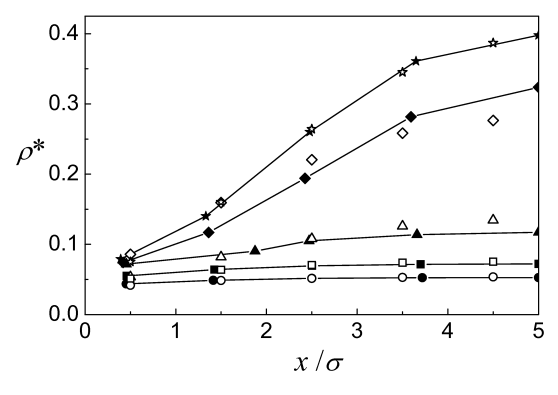
Figure 1: Density profiles for a $n$=9 layer model of a confined fluid in a slit pore (solid symbols). The temperature is $\mathit{T}^{\ast}$=1.0 and the wall separation is $\mathit{L}$=10$\sigma$, with mean densities $\rho^{\ast}$=1/20 (circles), 1/15 (squares), 1/10 (triangles), 1/5 (diamonds), and $\frac{1}{4}$ (stars). Open symbols represent the Monte Carlo simulations.

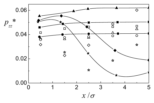
Figure 2: $\mathit{zz}$ pressure tensor component. Captions as in Fig. 1.

In Figs. 1 and 2, the density profiles and $\mathit{zz}$ components of the pressure tensor are shown for $\mathit{T}^{\ast}$=1 and $\mathit{L}$=10$\sigma$. The mean densities studied are $\rho^{\ast}$=1/20, 1/15, 1/10, 1/5, and 1/4. The agreement of the theoretical density profiles with the Monte Carlo simulations is very good. For the pressure there is a rather good correspondence for low densities, up to $\rho^{\ast}$=1/10. For the higher densities, differences appear, though the tendencies are similar. The discrepancies come first from the low density approximations done to get the Helmholtz energy. But, while in the simulation slab particles fluctuate and at higher densities some clusterization occurs, in the theory each layer is supposed to have a homogeneous density which makes it hard for the theoretical pressures to follow those obtained by simulation. For the density profiles, averaging the number of particles in each slab evidently compensates the clusterization, and the theory gives good results, at least for the rather low densities studied. The same picture applies to the behavior of the system for $\mathit{T}^{\ast}$=1 and $\mathit{L}$=15$\sigma$, at mean densities $\rho^{\ast}$= 1/10, and 1/5, represented in Figs. 3 and 4.

The results, as expected for hard repulsive walls, show a low density region next to the walls and an increasing density profile, with a maximum at the center of the slit pore. This behavior is also shown with density functional theory [1] and in other Monte Carlo simulations [2].

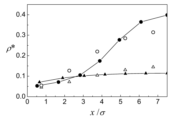
Figure 3: Density profiles for a $n$=13 layer model of a confined fluid in a slit pore (solid symbols). The temperature is $\mathit{T}^{\ast}$=1.0 and the wall separation is $\mathit{L}$=15$\sigma$, with mean densities $\rho^{\ast}$=1/10 (triangles), and 1/5 (circles). Open symbols represent the Monte Carlo simulations.

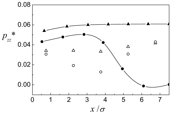
Figure 4: $\mathit{zz}$ pressure tensor component. Captions as in Fig. 3.

Finally, the good agreement of the theory with the experiment can be seen in the results shown in Fig. 5. In this figure, the excess number of molecules per unit area of pore surface $\Gamma$ is plotted in function of the external pressure,   at $T^{\ast}$=3.18 and $L$=4$\sigma$. These parameters approximate the experimental values [19] $T$=303 K and $L$=1.45 nm, if $\varepsilon/k=95.2$ K and $\sigma=3.75$ Å are used to characterize the nitrogen. In this case, due to the size of the sample, $n$=3 layers have been used for calculation. $\Gamma$ is defined as

$$\Gamma=\frac{N-N_{g}}{S}=(\rho^{\ast}-\rho_{g}^{\ast})\frac{L}{\sigma^{3}}$$ (13)

where $N_{g}$/$\rho_{g}^{\ast}$ is the number/density of particles which would occupy the slit pore in the absence of the adsorption forces. $\rho_{g}^{\ast}$ and the external pressure are determined equating the chemical potential inside the slit pore (Eq. 12) to the chemical potential coming from the bulk van der Waals equation at the same temperature. The theoretical results presented here are similar to the numerical simulation results obtained by the same authors who have done the experiment [19]. They assume that the differences at higher pressures could be a consequence of the uncertainty in the determination of the pore geometry.

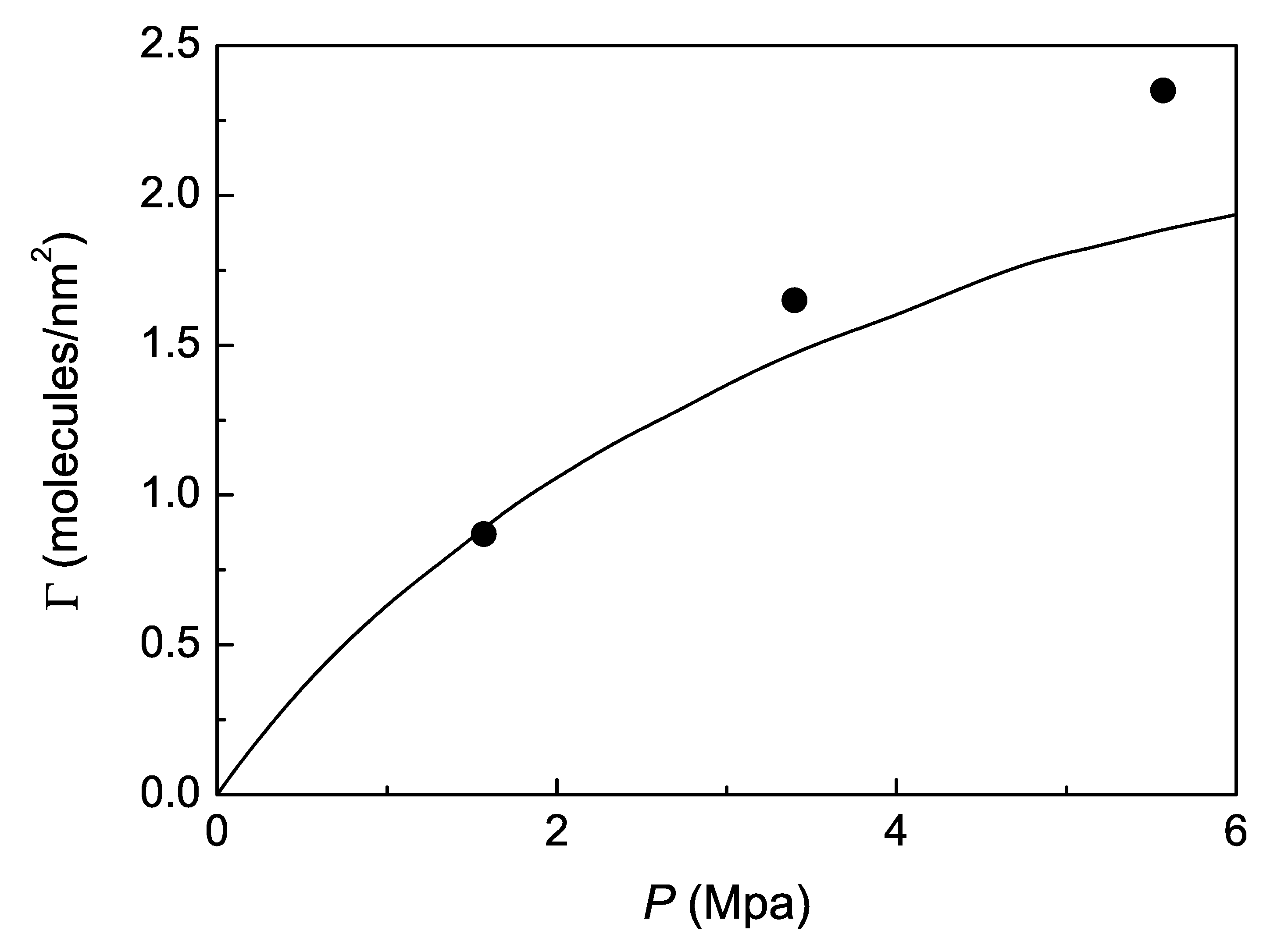
Figure 5: Excess number of molecules per unit area of pore surface $\Gamma$ as function of the external pressure. The full line represents the experiment (digitalized from Ref. [19]), and the dots are our theoretical results.

5 Conclusions

The application of a simple theory, with van der Waals-like approximations to the Helmholtz energy, to a particular model of spatial distribution makes it possible to obtain analytical expressions for the thermodynamic quantities. The study of a confined fluid in a slit pore geometry with a multilayer approximation produces good results when compared with Monte Carlo simulations at low densities. The agreement with a particular experiment on nitrogen confined in a graphite slit pore is remarkable, even though an excess quantity is in study. It may be concluded that the confinement reduces the importance that higher virial contributions have on the equation of the state of the confined fluid. Classical density functional theory [22] can also be applied to study the slit pore geometry, with very good agreement with experiments and simulations. Though the theoretical work developed in these pages is not a competitor of density functional theory, it has the advantages of having analytical expressions, and the possibility of easily introducing two immiscible components: for instance one or two layer lubricants wetting the walls and a gas or a liquid filling the rest of layers forming the capillary volume.

Appendix A

Expressions of quantities used in Eqs. 5–8:

$\begin{array}[]{l}{b=\frac{2}{3}\pi;B_{i}=\frac{\pi}{4}\frac{\sigma}{L_{xi}};A_{i}=a_{1}+\frac{a_{2}}{L_{xi}}+\frac{a_{3}}{L_{xi}^{3}}+\frac{a_{4}}{L_{xi}^{9}}}\\ \\ {a_{1}=-\frac{16}{9}\pi;a_{2}=\frac{3}{2}\pi;a_{3}=-\frac{1}{3}\pi;a_{4}=\frac{1}{90}\pi}\hskip 5.0pt(A1)\end{array}$

A correction has been made to get good critical parameters for the bulk ($\mathit{L\rightarrow\infty}$). For Argon $\mathit{a}_{1}$= -5.7538 and $\mathit{b}$=1.3538, and for nitrogen $\mathit{a}_{1}$= -1.5955 and b=1.0349.

$\begin{array}[]{l}{A_{i,\,i+1}=\frac{\pi}{90}\Bigl{[}-\frac{1}{L_{xi}^{9}}-\frac{1}{L_{xi}L_{xi+1}^{8}}+\frac{1}{L_{xi}(L_{xi}+L_{xi+1})^{8}}\Bigr{]}}\\ \hskip 30.00005pt-\frac{\pi}{3}\Bigl{[}-\frac{1}{L_{xi}^{3}}-\frac{1}{L_{xi}L_{xi+1}^{2}}+\frac{1}{L_{xi}(L_{xi}+L_{xi+1})^{2}}\Bigr{]}\\ \hskip 30.00005pt-\frac{3}{2}\frac{\pi}{L_{xi}}\hskip 130.0002pt(A2)\end{array}$

$\begin{array}[]{l}A_{i,\,i+2}=\frac{\pi}{90}\Bigl{[}\frac{1}{L_{xi+1}^{8}}-\frac{1}{(L_{xi}+L_{xi+1})^{8}}\\ \hskip 30.00005pt-\frac{1}{(L_{xi+1}+L_{xi+2})^{8}}+\frac{1}{(L_{xi}+L_{xi+1}+L_{xi+2})^{8}}\Bigr{]}\frac{1}{L_{xi}}\\ \hskip 30.00005pt-{\frac{\pi}{3}\Bigl{[}\frac{1}{L_{xi+1}^{2}}-\frac{1}{(L_{xi}+L_{xi+1})^{2}}-\frac{1}{(L_{xi+1}+L_{xi+2})^{2}}}\\ \hskip 30.00005pt{+\frac{1}{(L_{xi}+L_{xi+1}+L_{xi+2})^{2}}\Bigr{]}\,\frac{1}{L_{xi}}}\hskip 50.00008pt(A3)\end{array}$

$\begin{array}[]{l}{A_{i,\,i+3}=\frac{\pi}{90}\Bigl{[}\frac{1}{(L_{xi+1}+L_{xi+2})^{8}}}\\ \hskip 30.00005pt-\frac{1}{(L_{xi}+L_{xi+1}+L_{xi+2})^{8}}\\ \hskip 30.00005pt-\frac{1}{(L_{xi+1}+L_{xi+2}+L_{xi+3})^{8}}\\ \hskip 30.00005pt+{\frac{1}{(L_{xi}+L_{xi+1}+L_{xi+2}+L_{xi+3})^{8}}\Bigr{]}\frac{1}{L_{xi}}}\\ \hskip 30.00005pt-{\frac{\pi}{3}\Bigl{[}\frac{1}{(L_{xi+1}+L_{xi+2})^{2}}-\frac{1}{(L_{xi}+L_{xi+1}+L_{xi+2})^{2}}}\\ \hskip 30.00005pt{-\frac{1}{(L_{xi+1}+L_{xi+2}+L_{xi+3})^{2}}}\\ \hskip 30.00005pt+{\frac{1}{(L_{xi}+L_{xi+1}+L_{xi+2}+L_{xi+3})^{2}}\Bigr{]}\,\frac{1}{L_{xi}}}\hskip 20.00003pt(A4)\end{array}$

References

- [1] S A Sartarelli, L Szybisz, Correlation between asymmetric profiles in slits and standard prewetting lines, Pap. Phys. 1, 010001 (2009); L Szybisz, S A Sartarelli, Density profiles of Ar adsorbed in slits of CO2: Spontaneous symmetry breaking revisited, J. Chem. Phys. 128, 124702 (2008).
- [2] M Schoen, Computer Simulation of Condensed Phases in Complex Geometries (Lecture Notes in Physics), Springer, Berlin (1993).
- [3] M Schoen, Structure and phase behavior of confined soft condensed matter, In: Computational Methods in Surface and Colloid Science, Ed. M Borowko, Pag. 1, Marcel Dekker, New York (2000).
- [4] S Dietrich, Fluids in contact with structured substrates, In: New Approaches to Problems in Liquid State Theory, Eds. C Caccamo, J P Hansen, G Stell, Pag. 197, Kluwer, Dordrecht (1999).
- [5] J P R B Walton, N. Quirke, Capillary Condensation: A Molecular Simulation Study, Mol. Simul. 2, 361 (1989).
- [6] L D Gelb, K E Gubbins, R Radhakrishnan, M Sliwinska-Bartkowiak, Phase separation in confined systems, Rep. Prog. Phys. 62, 1573 (1999).
- [7] A Maciolek, A Ciach, R Evans, Critical depletion of fluids in pores: Competing bulk and surface fields, J. Chem. Phys. 108, 9765 (1998).
- [8] A Maciolek, R Evans, N B Wilding, Effects of weak surface fields on the density profiles and adsorption of a confined fluid near bulk criticality, J. Chem. Phys. 119, 8663 (2003).
- [9] P B Balbuena, K E Gubbins, Classification of adsorption behavior: simple fluids in pores of slit-shaped geometry, Fluid Phase Equilib. 76, 21 (1992).
- [10] P B Balbuena, K E Gubbins, Theoretical interpretation of adsorption behavior of simple fluids in slit pores, Langmuir 9, 1801 (1993).
- [11] O Pizio, A Patrykiejew, S Sokolowski, Phase Behavior of Lennard-Jones Fluids in Slit-like Pores with Walls Modified by Preadsorbed Molecules: A Density Functional Approach, J. Phys. Chem. C 111, 15743 (2007).
- [12] G J Zarragoicoechea, V A Kuz, van der Waals equation of state for a fluid in a nanopore, Physical Review E 65, 021110 (2002).
- [13] G J Zarragoicoechea,V A Kuz, Critical shift of a confined fluid in a nanopore, Fluid Phase Equilib. 220, 7 (2004).
- [14] M Schoen, D J Diestler, Liquid-vapor coexistence in a chemically heterogeneous slit-nanopore, Chem. Phys. Letters 270, 339 (1997).
- [15] R Defay, I Prigogine, Surface Tension and Adsorption, Longmans, London (1966).
- [16] R Defay, I Prigogine, Surface tension of regular solutions, Trans. Faraday Soc. 46, 199 (1950)).
- [17] T Murakami, S Ono, M Tamura, M Kurata, On the theory of surface tension of regular solution, J. Phys. Soc. Japan 6, 309 (1951).
- [18] L D Landau, E M Lifshitz, Física Estadística, Reverté, Barcelona (1969), pp. 269–273.
- [19] K Kaneko, R F Cracknell and D Nicholson, Nitrogen Adsorption in Slit Pores at Ambient Temperatures: Comparison of Simulation and Experiment, Langmuir 10, 4606 (1994).
- [20] M Schoen, D J Diestler, Analytical treatment of a simple fluid adsorbed in a slit-pore, J. Chem. Phys. 109, 5596 (1998).
- [21] M P Allen, D J Tildesley, Computer Simulation of Liquids, Oxford University Press, London (1987), Pag. 46–47.
- [22] J Wu, Density Functional Theory for chemical engineering: from capillarity to soft materials, AIChe J. 52, 1169 (2006).