Automatic unsupervised classification of all SDSS/DR7 galaxy spectra

Abstract

Using the k-means cluster analysis algorithm, we carry out an unsupervised classification of all galaxy spectra in the seventh and final Sloan Digital Sky Survey data release (SDSS/DR7). Except for the shift to restframe wavelengths, and the normalization to the $g$-band flux, no manipulation is applied to the original spectra. The algorithm guarantees that galaxies with similar spectra belong to the same class. We find that 99% of the galaxies can be assigned to only 17 major classes, with 11 additional minor classes including the remaining 1%. The classification is not unique since many galaxies appear in between classes, however, our rendering of the algorithm overcomes this weakness with a tool to identify borderline galaxies. Each class is characterized by a template spectrum, which is the average of all the spectra of the galaxies in the class. These low noise template spectra vary smoothly and continuously along a sequence labeled from 0 to 27, from the reddest class to the bluest class. Our Automatic Spectroscopic K-means-based (ASK) classification separates galaxies in colors, with classes characteristic of the red sequence, the blue cloud, as well as the green valley. When red sequence galaxies and green valley galaxies present emission lines, they are characteristic of AGN activity. Blue galaxy classes have emission lines corresponding to star formation regions. We find the expected correlation between spectroscopic class and Hubble type, but this relationship exhibits a high intrinsic scatter. Several potential uses of the ASK classification are identified and sketched, including fast determination of physical properties by interpolation, classes as templates in redshift determinations, and target selection in follow-up works (we find classes of Seyfert galaxies, green valley galaxies, as well as a significant number of outliers). The ASK classification is publicly accessible through various websites.

1. Introduction

The nebulae are so numerous that they cannot be studied individually. Therefore, it is necessary to know whether a fair sample can be assembled from the most conspicuous objects and, if so, the size of the sample required (Hubble 1936, Chapter II). Even though these arguments are from the outset of extragalactic astronomy, and they refer to the morphological classification of galaxies, the reasons put forward by Hubble remain valid today. The need to sort out and simplify justify all recent efforts to classify the spectra of galaxies (§ 1.1), including the present work. Such attempts are now more significant than ever since we have never had the large catalogs of galaxy spectra available today.

The seventh and final Sloan Digital Sky Survey data release (SDSS/DR7) provides spectra of some 930000 galaxies (Stoughton et al. 2002; Abazajian et al. 2009, and also the SDSS Web site). This uniform data set offers a unique opportunity to comprehensively classify the different spectra existing among nearby galaxies. Our paper presents the results of an unsupervised spectral classification of all the catalog. Unsupervised implies that the algorithm does not have to be trained. It is autonomous and self-contained, with minimal subjective influence. Thus, we deliberately avoid the use of physical constraints, or other a priori knowledge. We classify all galaxies simultaneously, requesting that galaxies with similar rest-frame spectra belong to the same class. This approach is in the vein of the rules for a good classification discussed by Sandage (2005), where he points out that physics must not drive a classification. Otherwise the arguments become circular when the classification is used to drive physics. The k-means algorithm that we implement is commonly employed in data mining, machine learning, and artificial intelligence (e.g., Everitt 1995; Bishop 2006), but it has been seldom applied in astronomy (see, however, Sánchez Almeida & Lites 2000). From the point of view of the algorithm, the galaxy spectra are vectors in a high-dimensional space, where they are distributed among a number of cluster centers. Each vector is assigned to the cluster whose center is nearest, and the center is the average of all the points in the cluster. It works iteratively. Starting from guess cluster centers, the spectra are assigned to their nearest centers, and then the centers are re-computed until convergence is reached. (Further details are given in § 2.) We choose it because of its extreme computational simplicity, as required to deal with large data sets (§ 2), and because it turned out to work very well in the first case we attempted. To our surprise, the algorithm managed to separate spectra of galaxies in the green valley within a collection of dwarf galaxies encompassing the full range of spectral types (Sánchez Almeida et al. 2009, § 3.1). Therefore, we found it natural to test the ability of k-means to distinguish among all kinds of galaxy spectra, and the success of this follow-up exercise is precisely the work reported here. In addition to the above virtues, the k-means method provides a prototypical high signal-to-noise spectrum for each class of galaxy, being the spectra of the galaxies in a class similar to the associated prototypical spectrum. These few representative spectra can be studied and characterized in detail as if they were individual galaxies, and then their properties can be attributed to all class members (§ 10). Other popular classification methods lack this powerful and convenient feature (see § 1.1).

The acronym ASK stands for Automatic Spectroscopic K-means-based, and it is used throughout the text to denote our classification. The paper is structured as follows. § 1.1 provides an overview of the main spectral classification methods employed so far. It also summarizes systematic trends resulting from the application of those methods. Our k-means classification algorithm is examined in § 2, where we test the class recovery upon known classes (§ 2.1), we analyze the repeatability of the classification (§ 2.2), and we assign probabilities to class membership (§ 2.3). The SDSS/DR7 dataset is briefly introduced in § 3. The actual classification of SDSS/DR7 is described in § 4. The ASK classification  is compared with Principal Component Analysis (PCA) classification in § 5 (see also § 1.1). The self-consistency of the ASK classification is discussed in various sections dealing with specific results; relationship between ASK class and Hubble type (§ 6), ASK class and color sequence (§ 7), ASK class and AGN activity (§ 8), and ASK class and redshift (§ 9). Further applications of the classification procedure are sketched in § 10. The ASK classification is publicly available as we explain in § 11. This section also outlines ongoing works based on ASK.

1.1. Spectral classification of galaxies

The first spectral classifications of galaxies are almost coeval with the discovery of the Hubble sequence. Hubble (1936) discusses how the spectral types and colors systematically vary within the morphological sequence, being ellipticals the reddest and open spirals the bluest (see also Humason 1931). One of the early attempts to set up an spectroscopic classification of galaxies is that by Morgan & Mayall (1957). They assign the blue part of the visible spectrum (3850 Å – 4100 Å) to stellar classes from A to K. They find a clear relationship between spectral class and shape, with the most concentrated galaxies (E, S0) belonging to class K, and the most diffuse galaxies (Sc, Irr) included in class A. The relationship applies to some 80% of the galaxies, a percentage probably larger for the targets of highest luminosity. Aaronson (1978) shows how the visible and IR colors of galaxies along the Hubble sequence can be understood as a one parameter family, in terms of the superposition of spectra of A0V dwarf stars and M0III gigant stars. Bershady (1995) points out that a simple model consisting of two stellar spectral types can reproduce the observed broad band colors, but only if the spectral types are allowed to vary. Five primary spectral types result from this modeling. Similar conclusions are also reached by Zaritsky et al. (1995) using stellar spectrum fitting.

Principal Component Analysis (PCA) is probably the most popular classification method employed so far. Each spectrum is decomposed as a linear superposition of a small number of eigenspectra, so that a few coefficients in this expansion (eigenvalues) fully describe the spectrum. It is fairly fast and robust, and a solid mathematical theory supports it (Everitt 1995). To the best of our knowledge, the first applications of PCA in this field have to do with stellar classification (e.g., Deeming 1964; Whitney 1983), then moved to quasar spectra (e.g., Mittaz et al. 1990; Francis et al. 1992), and finally arrived to the spectral classification of regular galaxies (e.g., Sodré & Cuevas 1994; Connolly et al. 1995). PCA is the method of reference, and we compare it in § 5 with our k-means. Two general results are common to all PCA analyses. Spectrumwise, galaxies can be characterized and distinguished by means of a single parameter that links the coefficients of the two or three first eigenspectra. Then different classes are obtained by splitting (somewhat artificially) this 1-dimensional family into pieces. The approach holds for 2dF galaxies (Folkes et al. 1999; Madgwick 2003), for galaxies in Kennicutt (1992) (Connolly et al. 1995; Sodre & Cuevas 1997), for Las Campanas Redshift Survey galaxies (Bromley et al. 1998), for DEEP2 galaxies (Madgwick et al. 2003), for IUE galaxies (Formiggini & Brosch 2004), and for SDSS (Yip et al. 2004). The second common result is the correspondence between spectral sequence and Hubble type. Even though ellipticals tend to be red and spirals tend to be blue, such relationship has a large intrinsic scatter (Connolly et al. 1995; Sodre & Cuevas 1997; Ferreras et al. 2006), which augments towards the UV (Formiggini & Brosch 2004). Sometimes elliptical galaxies with blue colors are found in the local universe (e.g., Kannappan et al. 2009), and this deviation from the trend is expected to grow even further with increasing redshift if, as Conselice (2006) argues, it is a coincidence that Hubble types correlate with colour in the nearby universe. At higher redshifts morphologically classified ellipticals are often blue in colour and actively forming stars (Conselice 2006; Huertas-Company et. al. 2009).

Despite the advantages mentioned above, PCA presents a clear drawback. It does not provide prototypical spectra to characterize the classes. The PCA eigenspectra do not resemble any member of the data to be classified and, in general, eigenspectra are of difficult physical interpretation (e.g., Chan et al. 2003; Formiggini & Brosch 2004; Yip et al. 2004). The advantage of having classes characterized by prototypical spectra is clear. These few spectra can be studied in detail using standard diagnostic techniques developed for individual galaxies through the years. Then the attributes of the prototypical spectra can be passed on to the class members, or they can be used as intermediate grid-points to interpolate the properties of the class members (see § 10). Moreover, the differences between a particular galaxy and its class prototype allow for precise relative measurements. In an attempt to complement PCA with this feature, Chan et al. (2003) developed an archetypal analysis algorithm. As the authors explain, it is like PCA but the eigenspectra are required to be members or mixtures of members of the input data set. However, by construction, the eigenspectra are extreme data points lying on the data set outskirts. Although physically meaningful, the eigenspectra are outliers, and it may be difficult to connect their physical properties with those of typical galaxy spectra. Other improvements on the basic PCA technique are local linear embedding (Vanderplas & Connolly 2009), and ensemble learning independent component analysis (Lu et al. 2006). These extensions are computationally expensive, and so far they have been introduced only as proof-of-concept works.

In addition to the superposition of stellar spectra and the PCA techniques described above, galaxies have been classified using neuronal networks (Folkes et al. 1996; Madgwick 2003), massive lostless data compression (Reichardt et al. 2001), information bottleneck (Slonim et al. 2001), and probably others. The algorithms have flourished in response to the availability of new large spectral databases. We are still in an expanding phase, which should lead to a final convergence of the various techniques. The different methods seem to roughly coincide in the global picture, but it is so far unclear whether they agree in the details.

2. The classification algorithm

In the context of classification algorithms, galaxy spectra are vectors in a high dimensional space, with as many dimensions as the number of wavelengths in use. The galaxy catalog to be classified is a set of vectors in this space, and so the (Euclidean) distance between any pair of them is well defined. Vectors (i.e., spectra) are assumed to be clustered around a number of cluster centers. The classification problem consists in (a) finding the number of clusters, (b) finding the cluster centers, and (c) assigning each galaxy in the catalog to one of these centers. We employ the k-means algorithm to carry out this classification (see, e.g., Chapter 5 in Everitt 1995; Bradley & Fayyad 1998; Sánchez Almeida et al. 2009). In the standard formulation, it begins by selecting at random from the full data set a number $k$ of template spectra. Each template spectrum is assumed to be the center of a cluster, and each spectrum of the data set is assigned to the closest cluster center (i.e., that of minimum distance or, equivalently, closest in a least squares sense). Once all spectra in the dataset have been classified, the cluster center is re-computed as the average of the spectra in the cluster. This procedure is iterated with the new cluster centers, and it finishes when no spectrum is re-classified in two consecutive steps. The number of clusters $k$ is arbitrarily chosen but, in practice, the results are insensitive to such selection since only a few clusters possess a significant number of members, so that the rest can be discarded. On exit, the algorithm provides a number of clusters, their corresponding cluster centers, as well as the classification of all the original spectra now assigned to one of the clusters.

The algorithm is simple and fast, as required to treat large data sets. It assures that galaxies with similar spectra end up in the same cluster, and provides cluster centers, i.e., prototypical spectra representative of all the galaxies in a cluster. In addition, it seems to work very well separating galaxy spectra, as inferred from the first test (see § 1), and from this work. Unfortunately, it has a major drawback. It yields different clusters with each random initialization. After pondering pros and cons, we decided to carry on with the algorithm, but not without evaluating the impact of the initialization on the classification. The impact is quantified and controlled through three complementary methods: (1) carrying out different random initializations and comparing their results, (2) assigning galaxies to several classes, each one with its own probability, and (3) trying alternative methods of initialization. The first point is dealt with in § 2.1 and § 4, leading to classifications whose classes share some 70% of the galaxies. It is not 100% because of spectra lying in between classes. This difficulty is to some extent cured by the second point, treated in § 2.3, which allows us to assign galaxies to several classes and, therefore, to identify galaxies in class borders. The third point is treated in the next paragraph, concluding that the scatter in the classification is not significantly modified by the mode of initialization. It does modify the timing, though.

We tried several initialization methods, including the standard one, that by Bradley & Fayyad (1998), and others (Peña et al. 1999). None of them seem to reduce the scatter due to the initial random seed (§ 2.1 and § 4). This behavior can be understood in terms of the existence of borderline galaxies, as argued in Appendix A. A proper initialization, however, reduces the iterations required to converge, and speeds up the procedure. We have adopted our own method, which is simple and fast, and it starts off with a reduced number of classes. It tries to select initial cluster centers according to the clusters that exist in the data set. If initial centers are purely chosen at random, then the clusters having the largest number of elements are overrepresented, and minor clusters may be even absent. The procedure works as follows: (Step 1) choose at random a small set of initial cluster centers (say, 10). (Step 2) Run one iteration of the standard k-means, and select as initial cluster center the cluster center with the largest number of elements. (Step 3) Remove from the set of galaxies to be classified those belonging to the selected cluster center. (Step 4) Go to step 1 if galaxies are still left; otherwise end. In addition to this particular initialization, we tuned the standard k-means described above with one extra ingredient. The iteration loop ends when the classifications in two successive steps are sufficiently close one another, i.e., when 99% of the assignations do not vary between two iterations. This simplification speeds up the convergence since the classification of the remaining 1% takes a long time, and does not help finding the main galaxy classes, already well characterized by 99% of the sample.

2.1. Testing the repeatability of the classification

Two classifications of the same data set are identical if they include the same galaxies in each class. With this criterion in mind, we compare two different classifications by pairing their two sets of classes according to the number of galaxies that they have in common. We compute the number of galaxies in common between each pair of classes formed by one class from one classification and the second class from the second classification. The two classes sharing the largest number of galaxies are assumed to be equivalent. The same criterion is repeated until all the classes of one of the classifications have been paired. Since the number of classes in the two classifications are not necessarily the same, some classes remain unpaired. This procedure tries to maximize the number of galaxies sharing the same class in the two classifications. We use the percentage of galaxies in equivalent classes as a measurement of the agreement between the two classification, dubbing it coincidence rate.

A first series of tests to check repeatability has been carried out using the 21493 quiescent blue compact dwarf galaxies (QBCD) selected by Sánchez Almeida et al. (2009) from SDSS/DR6. Here we employ the same wavelength windows used in Sánchez Almeida et al. (2009; they are labeled as QBCD in Table 1). Thirty independent classifications of this data set yield a coincidence rate of $71\pm 9$ %, with the error bar being the standard deviation. We think that the origin of these fluctuations in the number of common galaxies is due to the random initialization coupled with the large number of variables defining the spectra; see Appendix A. This 70% coincidence has two consequences. (1) A galaxy chosen at random from the sample has a 70% chance of appearing in equivalent classes in two different runs of the classification. (2) The cluster centers are very well defined since, independently of the initialization, they share 70% of the galaxies that define them. The coincidence of the final classification of SDSS/DR7 is similar (but a bit smaller), as it is discussed in detail in § 4.

2.2. Testing the class recovery upon known classes

We construct a set of mock observations to see whether the algorithm is able to recover clusters imposed on the data. To a data set of 21493 spectra (same number as in § 2.1), we add different amounts of pixel-to-pixel uncorrelated random noise. The 21493 spectra were randomly selected among three real spectra representative of galaxies along the color sequence in the blue cloud, the red sequence, and the green valley (see § 7). This 3-class mock observation encompasses the full range of spectra to be expected. When no noise is added, the algorithm returns 3 classes, with 100 % coincidence between the original and the classified spectra. As the noise increases, the number of recovered classes increases too. The fact that new classes have appeared does not mean that the algorithm is malfunctioning. Actually, the algorithm seems to be classifying the noise. When the signal-to-noise ratio per pixel is $\simeq\,$10, which is typical of SDSS spectra, one retrieves some 10 classes. However, the spectra of the different original classes are never mixed up, i.e., they end up in separate classes. The noise artificially increases the number of classes, but it does not wash them out. Moreover, it is easy to figure out which classes are faked by this kind of random noise because, being pixel-to-pixel uncorrelated, it does not modify global properties of the spectra such as colors. Different classes with different colors are not artifacts created by noise.

2.3. Assigning several classes to each galaxy

Given a collection of galaxy spectra, the k-means algorithm infers a small set of classes or clusters, and assigns each spectrum to one of them. A number of reasons advice addressing the inverse problem too, i.e., assigning classes to individual spectra once the classes are known. This alternative is required to classify spectra not used in the classification, which turns out to be a practical case of major interest (e.g., § 4, § 6). In addition, the classification does not provide unique sharp classes. The results in § 2.1 suggest that a significant number of galaxies are in between classes, and this fact could be easily acknowledged and quantified with a procedure to estimate the probability that a given galaxy belongs to each one of the known classes. Borderline galaxies must fit in several classes with similar probabilities. A general procedure to carry out such multiple assignation is worked out in this section.

The distance of spectrum ${\bf s}=(s_{1},s_{2},\dots)$ to class center ${\bf c}=(c_{1},c_{2},\dots)$ is defined as,

$$d({\bf s}-{\bf c})=|{\bf s}-{\bf c}|=\big{[}\sum_{i}w_{i}\,(s_{i}-c_{i})^{2}\big{]}^{1/2},$$ (1)

where $s_{i}$ and $c_{i}$ are the values of the spectrum and the cluster center in the $i-$th wavelength pixel. The weights $w_{i}$ allow one to select a subset among the pixels defining the spectra, i.e.,

$$w_{i}=\cases{0,&in discarded wavelengths,\cr m^{-1},&in used wavelengths,}$$ (2)

with $m$ the total number of pixels where $w_{i}\not=0$. k-means selects as class center the average of all the spectra belonging to the class. Each one of these spectra has its own distance to the cluster center, so that the full set defines a distribution of distances to the cluster center for the spectra in the class. Let us call $f_{\bf c}(d)$ the probability density function (PDF) of such distribution, i.e., $f_{\bf c}(d)\,\Delta d$ is the probability of finding a galaxy in cluster c with a distance to the cluster center between $d$ and $d+\Delta d$. The chances that galaxy s belongs to cluster c can be estimated as the probability of finding galaxies in the cluster with distances equal or larger than $d({\bf s}-{\bf c})$, i.e.,

$$P({\bf s},{\bf c})=\int_{d({\bf s-c})}^{\infty}f_{\bf c}(x)\,dx.$$ (3)

Unfortunately, sorting the classes according to their $P({\bf s},{\bf c})$ may be inconsistent with the assignation of classes made by k-means. Given a galaxy spectrum, k-means assigns to it the class of minimum distance, i.e., the class ${\bf c}_{k}$ where $d({\bf s}-{\bf c}_{k})\leq d({\bf s-c})\,\forall\,{\bf c}$. However, there is no guarantee that the class of minimum distance coincides with the class of maximum probability, i.e., in general ${\bf c}_{k}\not={\bf c}_{p}$ with ${\bf c}_{p}$ defined so that $P({\bf s},{\bf c}_{p})\geq P({\bf s},{\bf c})\,\forall\,{\bf c}$. Consequently, the sorting of classes according to their probabilities cannot be used to order classes in a way that agrees with k-means. We circumvent the problem defining a merit function, based on probabilities, that can be used to judge the membership of a given galaxy to the various classes. As a main constraint, the class of minimum distance must have the largest merit, so that the ordering provided by this merit function agrees with the assignation made by the k-means algorithm.

We call such merit function quality. For a spectrum s, assigned by k-means to class ${\bf c}_{k}$, the quality of class ${\bf c}$ is defined as,

$$Q({\bf c},{\bf s},{\bf c}_{k})=\int_{d({\bf s-c})}^{\infty}f_{{\bf c}_{k}}(x)\,dx.$$ (4)

Given a spectrum, its membership to various classes is judged according to $Q$, with the class of largest $Q$ the main affiliation, the one of second largest $Q$, the second main, and so on. The sorting according to quality is actually a sorting according to distance to the cluster centers since,

$$Q({\bf c_{1}},{\bf s},{\bf c}_{k})\geq Q({\bf c_{2}},{\bf s},{\bf c}_{k})\Leftrightarrow d({\bf s-c_{1}})\leq d({\bf s-c_{2}}).$$ (5)

This property guarantees that the class of minimum distance has the largest quality and, therefore, the main class attending to its quality agrees with the k-means assignation. Equation (5) follows from Eq. (4) because $f_{\bf c}$ is always positive, and so, $Q$ is a monotonic decreasing function of $d({\bf s-c})$. In addition to conforming to k-means, the quality $Q$ has a number of practical properties. Due to the normalization of the PDFs,

$$\int_{0}^{\infty}f_{\bf c}(x)\,dx=1,$$ (6)

the quality is always comprised between zero, for no match, and one, for perfect match,

$$Q({\bf c},{\bf s},{\bf c}_{k})\rightarrow\cases{1,&when $d({\bf c-s})\rightarrow 0$,\cr 0,&when $d({\bf c-s})\rightarrow\infty$.}$$ (7)

The best quality, i.e., that of the class of minimum distance, admits a simple interpretation. It is just the probability that the galaxy belongs to this class because,

$$Q({\bf c}_{k},{\bf s},{\bf c}_{k})=P({\bf s},{\bf c}_{k}).$$ (8)

If the best quality is large, then there are high chances that the galaxy is part of the class. If the best quality is similar to the second best quality, then the galaxy is in between classes. If the best quality is very small ($\ll 1$), then the galaxy is an outlier, meaning that it does not fit into any of the main classes.

Computing qualities as explained above requires estimating the PDF for the distribution of distances within a class. This can be derived from the histogram of distances to the cluster center among the galaxies that k-means has included within the class. After several trials, we found out that the observed cumulative distribution of distances can be very well approximated as,

$$\int_{d}^{\infty}f_{\bf c}(x)\,dx\simeq a_{1}+a_{2}\,d+a_{3}\,\exp\big{[}-[(d-a_{4})/a_{5}]^{2}\big{]},$$ (9)

where the five free coefficients $(a_{1},\dots,a_{5})$ are determined by a non-linear least-squares fit of the empirical cumulative histogram of observed distances. Figure 1 shows one of such fits.

Figure 1.— Example of cumulative distribution function of distances to the class center. The symbols show the observed values whereas the solid line corresponds to the analytical representation used in the work. Distances are relative to the standard deviation.

Real qualities are represented in Fig. 2, which includes the results in one of the test classifications in § 2.1. Figure 2, top, shows scatter plots of the 2nd-best quality versus the best quality (top left), and the 3rd-best quality versus the best quality (top right). A significant number of galaxies appear not far from the border where the best and 2nd-best qualities are equal and, therefore, many galaxies lie in between classes. Figure 2, bottom, shows the histograms of those qualities. Note how the best quality has a rather flat distribution peaking at, say, 0.6. Note also how the number of galaxies with very small best quality is also very small. These are outliers whose spectra differ significantly from the characteristic spectra of the main classes.

Figure 2.— Top: example of scatter plot of quality versus quality. Top-left: 2nd-best quality versus best quality. Points not far from the diagonal can be classified as either one of the two classes. Top-right: 3rd-best quality versus best quality. Bottom: histograms of qualities for the best quality class (the solid line), the 2nd-best class (the dotted line), and the 3rd best class (the dashed line). Note that even the best qualities are sometimes close to zero, implying that these galaxies are outliers of the classification.

3. The data set: SDSS/DR7 spectra

The SDSS/DR7 is the final major data realease of the SDSS project. Details about SDSS and the DR7 can be found in, e.g., Stoughton et al. (2002), Abazajian et al. (2009), and also in the thorough SDSS website. The spectroscopic part of the survey contains some 930000 galaxy spectra, and this full set is classified in our work. The basic properties of spectrograph and spectra will be summarized here, but we refer to the references given above for further details. The SDSS spectrograph has two independent arms, with a dichroic separating the blue beam and the red beam at 6150 Å. It simultaneously renders a spectral range from 3800 Å to 9250 Å, with a spectral resolution between 1800 and 2200. The sampling is linear in logarithmic wavelength, with a mean dispersion of 1.1 Å pix^-1 in the blue and 1.8 Å pix^-1 in the red. Repeated 15 min exposure spectra are integrated to yield a S/N per pixel $>4$ when the apparent magnitude in the $g$-band is 20.2. The spectrograph is fed by fibers which subtend about 3″on the sky. Most galaxies are larger than this size therefore the fibers tent to sample their central regions (e.g., 88% of the galaxies have effective radii larger than half the fiber diameter).

Two adjustments are made on the original spectra before classification. First, they are brought to restframe wavelengths using the redshifts provided by SDSS. This wavelength shift involves an interpolation, and we take advantage of this need to bring to a common wavelength scale all spectra, as required by the classification algorithm. The common scale has the same number of pixels as the original spectra (3850), and it is equispaced in logarithmic wavelength from 3800 Å to 9250 Å. Obviously, the IR part of the spectrum is missing as the redshift increases, and we extrapolate it with a constant. Note, however, that this missing part is not used for classification (see below and § 4). The second manipulation is a global scaling applied after the resframe correction. The spectra are normalized to the flux in the $g$ color filter (effective wavelength $\simeq$ 4825 Å), a normalization factor that we compute for each spectra using the transmission curve provided by SDSS. This re-scaling automatically corrects for the flux dimming associated with the redshift (e.g., Blanton & Roweis 2007), but the original motivation was allowing comparison between galaxies of different absolute magnitudes. If the global scaling is not removed, the flux of the galaxy completely dominates the classification, and galaxies are split in bins of equal luminosity, rather than in spectral classes.

No further correction has been applied to the data. We do not correct for extinction, seeing, galaxy size, aperture bias, etc. This apparent sloppiness actually results from a deliberate attitude towards classification, following the guidelines by Sandage (2005) mentioned in § 1. If these corrections are important and the classification is working properly, then the spectra of the same type of galaxy with and without an uncorrected bias should appear in separate bins. It is then a matter of a posteriori physical interpretation to infer what causes the different classes, and eventually join some of them when appropriate.

4. Final implementation: the classification of SDSS/DR7

The spectra to be classified by k-means must share the same wavelength scale, i.e., the same sampling interval and the same wavelength range. SDSS/DR7 has a significant number of galaxies up to redshift 0.5 (see Fig. 3). At this redshift the reddest restframe wavelength that SDSS provides is 6200 Å, therefore, in order to use the full data set for classification, one should restrict the range of wavelengths down to 6200 Å. Alternatively, one can restrict the range of redshifts of the galaxies. We have chosen the second possibility to avoid overlooking in the classification lines as important as H$\alpha$. The full set of spectra described in § 3 has been divided into a low redshift part (redshift $\leq 0.25$, with 788677 spectra) and a high redshift part (redshift $>0.25$, with 138649 spectra). The low redshift part is classified by means of the k-means algorithm, which provides the classes. Then the high redshift part is classified according to the classes derived from the low redshift part using the tools developed in § 2.3. The reason for choosing 0.25 as the dividing redshift is twofold. First, the distribution of redshifts in SDSS/DR7 seems to present a discontinuous behavior at roughly this redshift (see Fig. 3, and also the discussion in § 9). Second, and most important, 0.25 is the largest redshift that allows us to include for classification the near-IR TiO bands characteristic of M stars – the reddest restframe wavelength at this redshift is some 7500 Å.

Figure 3.— Scatter plots of apparent $g$ magnitude (left) and absolute $g$ magnitude (right) versus redshift for the galaxies in the SDSS/RD7. The plots include only a fraction of the galaxies chosen at random to avoid overcrowding.

In addition to removing the reddest part of the spectrum missed by the redshift of the galaxies, several reasons advice using only selected bandpasses to carry out the classification. Including too much continuum does not add information but dilutes the signals contained in the spectral lines. The number of wavelengths in the spectra sets the dimensions of the vectors to be classified. The larger the number of wavelengths the more computationally demanding the classification, which makes it advisable limiting the number of wavelengths. Keeping these caveats in mind, we use for classification only the bandpasses shown as dotted lines in the bottom of Fig. 4, which are also listed in Table 1. Except for a near-IR window between 8400 Å and 8800 Å, they include all the bandpasses employed by Sánchez Almeida et al. (2009, § 3) in the classification that triggered the present work (see § 1). These bandpasses contain the main emission lines that trace activity (star formation and AGN activity). Since they are distributed along the visible spectrum, they also provide sensitivity to the colors of the galaxies. In addition, we include all the bandpasses of the Lick indexes, which were selected because they depend on the age and metallicity of the stellar content of the galaxies(Worthey et al. 1994; Worthey & Ottaviani 1997). Finally, we include two windows at the location of TiO bands characteristic of M stars and early type galaxies (at 7150 Å and 7600 Å). These bandpasses are sensitive to the level of the near-IR continuum, and are tracers of old stellar populations.

Figure 4.— Template spectra representing the major classes in the ASK classification of the SDSS/DR7 galaxies. The different spectra have been artificially shifted upward according to their $u-g$ color. (Otherwise the plot becomes overcrowded.) The numbers next to the spectra (in the left hand side of the plot) correspond to the class number, which was assigned according to the $u-g$ color (ASK  0 for the reddest, ASK  1 for the second reddest, and so on up to ASK  22). Gaps in the numbering indicate the presence of minor classes of intermediate colors. The fluxes are in dimensionless units, i.e., they are normalized to the average flux in the $g$-filter bandpass. Wavelengths are given in $\mu$m. The dotted line differs from zero at the wavelengths used for classification.

Table 1Bandpasses used in the ASK classification of SDSS/DR7

From – To	Comment
4000 – 4420	QBCD blue, H$\delta_{A}$, H$\delta_{F}$, CN1, CN2,
	Ca4227, G4300, H$\gamma_{A}$, H$\gamma_{F}$, Fe4383
4452 – 4474	Ca4455
4514 – 4559	Fe4531
4634 – 4720	Fe4668
4800 – 5134	QBCD green, H$\beta$, Fe5015, Mg1
5154 – 5196	Mg2, Mgb
5245 – 5285	Fe5270
5312 – 5352	Fe5335
5387 – 5415	Fe5406
5696 – 5720	Fe5709
5776 – 5796	Fe5782
5876 – 5909	Na D
5936 – 5994	TiO1
6189 – 6272	TiO2
6500 – 6800	QBCD red
7000 – 7300	TiO band
7500 – 7700	TiO band

Note. — Wavelengths are in Å. The Comment contains the names of the Lick indexes in the bandpass, plus additional information used to identify the bands in the main text.

Initially, the computer resources needed to carry out the classification were unclear. The procedure is iterative (§ 2), and the timing is mostly set by the number of iterations, which scales in a unknown fashion with the number of spectra and wavelengths ($788677\times 1637$). An exploratory procedure was written in Interactive Data Language (IDL), and it turned out to be faster than expected since convergence occurs in, typically, less than 50 iterations. Using a 8-core Intel Xeon 2.66 GHz machine with 32 GB of RAM, 50 iterations last less than 300 minutes. (The access to sufficient RAM was critical, since the array with the spectra to be classified occupies some 11.6 GB.) Even if fast, the IDL code does not allow us to carry out the battery of classifications required to study the dependence of the classification on the random initialization (§ 2). Fortunately, the k-means algorithm can be parallelized, and we developed a second parallel version of the code using Fortran and the MPI (Message Passing Interface) library. The performance of the parallel version is good. The algorithm scales very well, so that adding more CPUs implies a near to linear reduction in the execution time. A hundred executions of the parallel code using a cluster of 48 Intel Xeon CPUs (2.4 GHz) takes of the order of 1 hour. This figure outperforms the IDL code by a factor of 500.

Aided with the parallel version of k-means, we carry out 150 independent classifications of the data set. Because of the random initialization, each one of these classifications differs (§ 2). Each run of the algorithm groups similar spectra in clusters so, in principle, all of them provide valid classifications. Then the problem arises as to which one of these classifications is best, i.e., which one should be chosen as the classification. Ideally, one would like to choose a classification (1) with a small number of classes, (2) being representative of all classifications, and (3) having small dispersion within the classes. Condition (1) is obvious and will not be discussed further. According to condition (2), we would like the classification to be as representative as possible of any other classification. Condition (3) demands that the spectra employed in deriving the classification are as close as possible to a class center spectrum. Figure 5 shows scatter plots of three numerical coefficients that we devised to quantify the three requirements above. Figure 5a and 5c include the average percentage of galaxies that a particular classification has in common with the other 149 classifications – it is just the percentage of galaxies in equivalent classes as defined in § 2.1, and it is labeled in the figures as coincidence. It spans between 62% and 71%. The coincidence is represented in Fig. 5a versus the average dispersion of the classification, which is just the mean of distance between galaxies and class centers defined in equation (1). The dispersion admits a simple interpretation: it is the typical difference per pixel between a spectrum in its class. (Because of the normalization, the spectra have their continuum at about one, therefore, dispersion 0.1 corresponds to differences of the order of 10%.) Note that there is no obvious correlation between the two parameters, but the classifications seem to cluster around two dispersions, the smallest being of the order of 0.16. Figure 5b shows the scatter plot between the number classes in a classification (classes altogether containing 99% of the galaxies) and the dispersion. Classifications having between 11 and 22 classes exist, with a typical value between 15 and 19. Again no obvious relationship between number of classes and dispersion is observed. Finally, Fig. 5c shows the scatter plot of coincidence versus number of classes. Attending to the three requirements above, we select those classifications having

1. less than 18 classes,

2. coincidence larger than 70%,

3. dispersion smaller than 0.17.

Figure 5.— Scatter plots with the three parameters characterizing the 150 different classifications from which we have drawn the final one in Fig. 4. (a) Percentage of galaxies common to all other classifications (coincidence) versus typical scatter of the spectra with respect to the class spectrum (dispersion). (b) Number of major classes versus dispersion. (c) Coincidence versus number of major classes. We select classifications having coincidence $>70\%$, dispersion $<0.17$, and 17 classes or less.

Four classifications fulfill these requirements. Lacking a better criterion, we choose one of them at random. The chosen classification turns out to have a coincidence of 70.8%, a dispersion of 0.16, and it has 28 classes, but 17 of them contain 99% of the galaxies. These 17 classes are denoted in the paper as major classes. The spectra of the major classes are shown in Fig. 4. They have been labeled according to the $u-g$ color, from the reddest, ASK  0, to the bluest, ASK  27. By using numbers to label the classes we are not implicitly assuming that the spectra represent a one dimensional family. The numbers are only tags to name the classes.

Figure 6a shows the colors characteristic of the ASK classes. The number of elements corresponding to each class is included in Fig. 6b. The horizontal dotted line in this figure indicates the threshold for major class, i.e., classes with a number of elements above this threshold contain 99% of the classified galaxies. Their spectra are those shown in Fig. 4. The main properties of all classes are summarized in Table 2.

Figure 6.— (a) Color versus ASK class number. Class numbers have been assigned according to the $u-g$ color of the template spectra, which explains the monotonous decrease of this color with class number. The larger the class number the bluer the galaxy. Colors $g-r$ and $r-i$ are also included as indicated by the inset. (b) Histogram of the number of galaxies existing in each class. The horizontal dotted line shows the threshold that separates major classes from the rest (i.e., classes having altogether 99% of the classified galaxies). The colors and number of members shown in these figures are listed in Table 2.

A blow up with the bluest part of Fig. 4 is included in Fig. 7, where some of the characteristic emission and absorption features are labeled. Note how the spectra vary gradually with the class number. Even the smallest ripples in these average spectra are real. Upon averaging, the signal-to-noise ratio is expected to increase as the square root of the number of class members. The major class with less members still has $\sim$ 5000 elements (Fig. 6b), which sets a lower limit to the S/N per pixel of $\sim 700$. The systematic change of global properties along the sequence is important to constrain the effects of noise on the number of classes (§ 2.1). Altough noise artificially increases the number of classes, it does not change in a systematic way global spectral properties such as colors. Except perhaps at the blue end of the classification, the colors of classes vary systematically along the sequence (Fig 6; see also § 7), which discard any significant influence of the random pixel-to-pixel uncorrelated noise on the number of classes.

Figure 7.— Zoom into the bluest wavelength range of Fig. 4. In addition to the lines and labels in the original figure, this plot also includes the most prominent spectral lines (vertical dashed lines with labels). For scaling, shifting, and further details, see the caption of Fig. 4.

Table 2Main properties of the ASK classes

ASK class	members	$u-g$	$g-r$	$r-i$	H$\beta$	[OIII]$\lambda 5007$	H$\alpha$	[NII]$\lambda$6583	% emission	Clustering
0∗	111447	1.59	0.91	0.44	-0.3	0.7	0.9	2.0	9	neutral
1∗	18032	1.57	1.05	0.53	0.3	1.1	2.9	3.2	29	neutral
2∗	213936	1.57	0.84	0.39	-0.4	0.4	0.1	1.3	2	good
3∗	80530	1.37	0.75	0.35	-0.7	0.6	0.7	1.6	8	neutral
4∗	20456	1.20	0.91	0.45	2.7	2.3	13.9	8.2	95	bad
5∗	68626	1.18	0.80	0.38	1.5	1.6	8.5	5.3	78	neutral
6∗	4669	1.17	0.77	0.34	3.5	29.6	14.2	10.9	98	good
7	1089	1.11	0.71	0.29	8.7	84.7	22.5	15.2	100	good
8	211	1.06	0.59	0.18	22.8	233.1	36.0	15.5	95	good
9∗	71671	1.00	0.68	0.32	2.4	1.6	12.0	5.8	89	neutral
10∗	32227	0.95	0.72	0.34	5.1	2.7	24.2	11.1	99	neutral
11∗	6369	0.91	0.78	0.33	9.7	5.4	42.2	19.8	100	good
12∗	51314	0.83	0.58	0.26	5.4	3.0	24.5	9.3	98	good
13∗	26705	0.81	0.50	0.24	2.6	3.0	11.2	3.9	81	bad
14∗	25026	0.72	0.52	0.21	10.2	6.1	45.7	16.1	99	good
15	68	0.70	-0.23	-0.57	176.4	743.5	715.3	14.1	25	good
16∗	26504	0.67	0.40	0.17	7.1	8.8	30.4	7.1	99	neutral
17	134	0.65	-0.15	-0.51	161.7	630.1	549.9	16.4	35	good
18∗	5687	0.61	0.48	0.13	19.5	18.5	83.9	24.9	100	good
19∗	12808	0.61	0.36	0.13	13.0	21.6	54.6	9.8	100	good
20	238	0.56	-0.03	-0.31	105.5	492.9	408.2	17.6	81	good
21	179	0.55	-0.03	-0.29	97.1	461.5	356.7	16.6	69	good
22∗	4781	0.55	0.28	0.08	19.8	48.3	82.5	9.7	100	good
23	2366	0.54	0.34	0.04	31.5	61.1	130.7	22.8	89	neutral
24	1910	0.51	0.22	0.00	34.5	106.6	148.5	12.9	98	good
25	488	0.51	0.08	-0.16	72.3	253.8	302.7	18.5	94	good
26	986	0.50	0.19	-0.07	51.7	159.9	219.3	19.6	100	good
27	199	0.48	0.13	-0.16	67.4	230.7	278.8	19.7	85	good

As we explained in the first paragraph of the section, the full set of galaxies was split into two parts. The low redshift part has been used to derive spectral classes, which automatically leads to its classification as explained above. Based on these classes, and using the procedure developed in § 2.3, we extended the classification to the high redshift subset. The use of the same classes is an assumption which, however, seems to be secure since the properties of the galaxies thus classified do not show any systematic difference with respect to the low redshift subset (see § 9). Moreover, the procedure in § 2.3 has been also applied to the low redshift part, already classified by k-means. It provides qualities for all classes, which permits identifying borderline galaxies and outliers, and it allows us deriving physical parameters by interpolation (§ 10).

The success of k-means does not imply the existence of well defined clusters in the 1637-dimensional classification space. As we discuss above, the separation between classes is not sharp. Galaxies are often close to the borders, which explains the variability between different realizations of the classification (§ 2.1). The presence of many borderline galaxies seems to imply a rather continuous distribution of points in the classification space, that k-means astutely partakes assuring the elements of each class to be similar. Generally speaking, classes should not be associated with true clusters in the classification space. However, some of the classes seem to represent genuine clusters as judged from the distribution of qualities. Qualities were introduced in § 2.3 to characterize the membership of each galaxy to the classes. Galaxies next to class borders have similar best quality and 2nd-best quality. Therefore, if the galaxies in a class are of this kind, then the class cannot portray a clear cluster. Conversely, classes corresponding to well defined clusters have their members separated from the other classes, i.e., their galaxies tend to have a best quality larger than the 2nd-best quality. This condition is met by some of the classes, indicating clustering. Thus we use the ratio between best and 2nd-best qualities to assign a degree of grouping to the different classes. Figure 8 shows histograms of the ratio between the best quality and the 2nd best quality for the major classes. Some of the histograms have a clear peak at a ratio significantly smaller than one, implying clustering (e.g., ASK 2). Other histograms present a flat distribution (e.g., ASK 0), whereas a minority of classes show most of their members having similar best and 2nd-best qualities (e.g., ASK 13). Attending to the shape of these histograms, the clustering of each class has been labeled as good, neutral or bad; see the last column of Table 2. Note that the clustering tends to be good or neutral rather than bad.

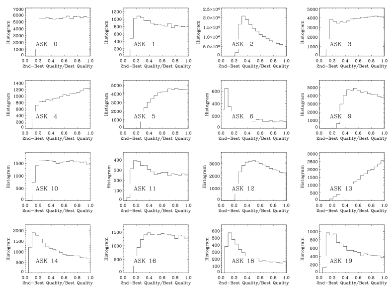
Figure 8.— Histograms of the ratio between the best and the 2nd-best qualities for the major classes. Those classes corresponding to proper clusters in the 1637-dimensional classification space should have a distribution of ratios peaking away from one (e.g., ASK 2). Only galaxies whose best quality is larger than 0.2 have been considered.

5. Relationship between ASK class and PCA classification

SDSS/DR7 already provides a spectral classification based on PCA, which is a linear expansion of each spectrum in terms of a small number of eigenspectra (§ 1). The eigenspectra for the SDSS expansion were derived from a subset of approximately 200000 galaxies, as explained by Yip et al. (2004). Following Connolly et al. (1995) and others, Yip et al. (2004) use a diagnostic plot to separate spectral classes based on the three first eigenvalues, $a_{1},a_{2}$ and $a_{3}$. Extreme emission galaxies, early type galaxies, and late type galaxies can be distinguished in the $\phi_{\rm KL}$ versus $\theta_{\rm KL}$ plane, where the two mixing angles are defined as

$$\phi_{\rm KL}= \arctan(a_{2}/a_{1}),$$ (10)

$$\theta_{\rm KL}= \arccos(a_{3}).$$ (12)

Figure  9 shows this diagnostic plot for all SDSS/DR7 galaxies, and for the major ASK classes separately.

Figure 9.— PCA diagnostic plot for 50000 randomly chosen galaxies in the SDSS/DR7. The full set is included in the top left panel, where we also mark the location of the early type (et), late type (lt) and extreme emission (ee) galaxies according to the separation in Yip et al. (2004). The other plots show the different major ASK classes individually (see the insets). Note how the ASK classes occupy well defined places in the PCA diagnostic plot. Given the ASK class of a galaxy, one can predict its location in the PCA plane. The opposite does not hold in general. All plots include the same contour indicating the boundaries of the full distribution. The two mixing angles $\theta_{\rm KL}$ and $\phi_{\rm KL}$ are given in degrees. Major classes 19 and 22 are not shown because they do not fit into the figure, but they follow the sequence.

We have used the PCA eigenvalues directly provided by SDSS/DR7. The ASK classes occupy well defined places in the PCA diagnostic plot, which implies that the PCA classification and the ASK classification are consistent. Given the ASK class of a galaxy, one can predict its location in the PCA plane. The opposite does not hold since some ASK classes overlap in the PCA diagnostic plot (cf. ASK 9 and ASK 10). The ASK classification is more refined; it simply includes more classes than PCA, therefore, the two classifications are consistent but not equivalent. The location of early type galaxies, late type galaxies, and extreme emission galaxies made by Yip et al. (2004) is also included in Fig. 9 (top left panel, symbols et, lt, and ee, respectively). One can see how this rough PCA based separation is also consistent with the ASK classes. There is a systematic trend to go from the location of the early types to the late types as the ASK class number increases. This behavior coincides with the trend to be derived from the morphological classification in § 6. The region of extreme emission galaxies deserves a separate comment. Note that the galaxies appearing in this region do not show up among the galaxies in the major classes included in Fig. 9. These extreme galaxies belong to the minor classes with high ASK class number (not shown), i.e., the bluest among the ASK classes. The points clearly outside the contour in Fig. 9 are partly included in the ASK classes next to them, and partly in additional minor classes (not shown). ASK 2 seems to be the only exception. It includes a few galaxies in the extreme emission region, and we have not been able to pin down the cause. However, the fact that ASK 2 shows more outliers then other classes is probably an artifact due to ASK 2 being the most common class (Table 2). If all classes include a similar fraction of outliers, they will be more conspicuous in scatter plots of ASK 2.

In short, although ASK is more refined, ASK and PCA seem to agree with small internal scattering. Moreover, the scatter between these two purely spectroscopic classifications is much smaller than the scatter in the ASK versus morphological classification analyzed in the next section.

6. Relationship between ASK class and Hubble type

The morphological type of a galaxy (Hubble type) is closely related to its spectrum, a relationship known for long (see § 1). The analysis of such relationship in the case of ASK is mandatory, and we will do it in a follow-up work where the morphology of a large number of galaxies is derived automatically (§ 11). However, in order to show the consistency of the ASK classification, we include here a preamble based on a limited number of galaxies which shows how early types are associated with small ASK numbers, and vice-versa.

We have ASK-classified the galaxies in the spectral atlas of Kennicutt (1992). He provides spatially integrated spectra (from 3650 Å to 7100 Å) of a set of 55 nearby galaxies with known Hubble types. The set contains all Hubble types, from gigant ellipticals (cD, NGC 1275) to dwarf irregulars (dI, Mkr 35). We assign each galaxy to the ASK class whose spectrum is closest to the galaxy spectrum as explained in § 2.3. The match between ASK template spectra and Kennicutt spectra is illustrated in Fig. 10, which contains representative spectra of an early type galaxy and a late type galaxy. These particular fits ignore the spectral regions with emission lines (see the weights shown as a dotted line in the figures).

Figure 10.— Two representative examples of the fits between ASK class spectra and galaxies in the atlas by Kennicutt (1992). Galaxy names, Hubble types, and ASK numbers are included in the insets. The dotted lines correspond to the weights used for fitting – wavelengths where the weight is zero have been ignored. Wavelengths are given in Å. Symbols and solid lines correspond to Kennicutt spectra and ASK class spectra, respectively.

The scatter plot of the assignation is shown in Fig. 11. It displays the Hubble type given by Kennicutt (1992) versus the ASK class for the galaxies in the atlas. (Actually, for 53 out of the 55 original galaxies, since Mrk 3 is not in the electronic catalog, and NGC 3303 has no clear Hubble type – it presents two nuclei undergoing a major merger.) Note the clear trend for the small ASK numbers to be associated with early types and vice-versa. The dividing line between early types (E,…S0) and late types (Sa, SBa,…I) seems to be about ASK  6, so that numbers smaller than this limit correspond to early types. The trend is even more clear if one ignores those galaxies classified as peculiar by Kennicutt (1992), which are shown in the figure as asterisks. However, one cannot ignore the large scatter in the figure – there is no one-to-one relationship between spectroscopic class and morphological class.

Figure 11.— Scatter plot of Hubble type versus ASK class for the galaxies in the atlas by Kennicutt (1992). The plot contains 53 out of the 55 galaxies in the atlas – Mrk 3 has no spectrum in the electronic catalog, and NGC 3303 belongs to an undefined class since it is undergoing a major merger. Note the clear trend for the small ASK class numbers to be associated with early types, and vice-versa. The trend is even more clear if one ignores those galaxies classified as peculiar by Kennicutt (1992) (the asterisks). However, one cannot ignore the scatter – there is no one-to-one relationship between spectroscopic class and morphological class. In order to avoid the overlapping of the galaxies with the same Hubble type and ASK class, we have added a small artificial random vertical shift to all points.

The conclusion that there is a general trend with large scatter is very much in the vein of all previous studies comparing spectroscopic and morphological classifications (e.g., Zaritsky et al. 1995; Conselice 2006, and § 1.1). Actually, the relationship between morphological and spectroscopic types gets fuzzier with increasing lookback time, and perhaps it disappears in the early Universe (Conselice 2006; Huertas-Company et. al. 2009).

We have repeated the above exercise using the eye-bold morphological classification presented by Fukugita et al. (2007). It is based on bright galaxies in a north equatorial stripe from SDSS/DR3, visually classified by three different observers based on $g$-band images. The catalog contains 2253 galaxies, but only 1866 targets have spectra and so overlap with our classification. We have also used this set to compare the morphological Hubble type and the ASK classification, with results similar to those for Kennicutt galaxies. There is a global trend with significant scatter. The size of the set allowed us to discard several observational bias that may cause the scatter. It is not due to misclassifications. The scatter is not reduced upon using only high quality ASK class determinations (quality $>0.8$; § 2.3), or when Im and peculiar galaxies are excluded from the sample. The scatter remains considering only small galaxies contained within the spectroscopic fiber ($<$ 1.5″ effective radius). The last test assures that the scatter is not produced by large spirals misclassified because the SDSS spectrum just samples their (red) bulge.

7. ASK classes and the bimodal color distribution

The colors of the galaxies follow a bimodal distribution (e.g., Strateva et al. 2001; Balogh et al. 2004; Baldry et al. 2004), with a red population (the red sequence), a blue population (the blue cloud), and the so-called green valley in between (e.g., Salim et al. 2007). The two main populations are believed to represent passively evolving red galaxies and blue star-forming galaxies, with galaxies in transition forming the green valley. As we explain in § 1, this work was partly triggered by the ability of k-means  to distinguish green valley spectra (Sánchez Almeida et al. 2009). Therefore, we found it necessary to discuss the location of the ASK classes in a plot where the red and the blue populations show up separately (e.g., Bershady et al. 2000; Strateva et al. 2001).

Figure 12 (top left panel) shows the distribution of all SDSS/DR7 galaxies in a $u-g$ versus $g-r$ plot. The image represents the 2-dimensional histogram of the distribution of colors. The concentrated spot at $g-r\simeq 0.8$ and $u-g\simeq 1.7$ corresponds to the red sequence. The blue cloud appears in this representation as an extended tail. The other panels in Fig. 12 show the different classes separately, and they all include the 2-dimensional histogram for reference. An inspection to Fig. 12 reveals a number of properties. First, the ASK classification separates galaxies into well located positions of the color-color plane. The red cloud is characterized by the most numerous class, ASK  2. ASK  0 and ASK  1 also belong to the red sequence, but to its outskirts. The blue cloud is split into several classes, starting with ASK  9 and continuing with higher ASK classes. In between these two groups, ASK  3, ASK  5 and ASK  6 populate the green valley – ASK  4 seems to be made of outliers of the main relationhip. As we originally presumed, the ASK classification separates galaxies in colors with a finesse to automatically pinpoint classes in the green valley. An in-depth analysis of the galaxies in these classes will be carried out in a follow-up work (see § 11).

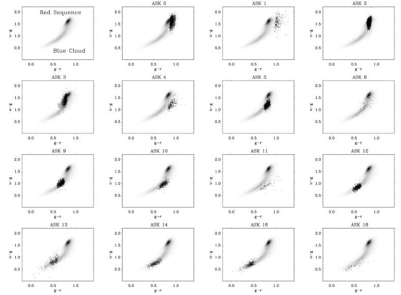
Figure 12.— Plots of $u-g$ versus $g-r$ for the galaxies belonging the major ASK classes. The top left panel contains an image with the 2-dimensional distribution of colors in the full SDSS/DR7. The remaining panels show the individual classes separately, as indicated in the labels, together with the 2-dimensional histogram for reference. Major classes 19 and 22 are not shown because they do not fit into the figure, but they follow the trend.

8. Relationship between ASK class and AGN activity

We have studied the position of our classes on the BPT diagram (named after Baldwin et al. 1981), which is commonly used to separate Active Galactic Nucleus (AGN) activity from normal star formation activity in galaxies with emission lines (e.g., Kauffmann et al. 2003). The diagnostic diagram consists of a scatter plot of the ratio of fluxes [OIII]$\lambda 5007/{\rm H}\beta$ versus [NII]$\lambda 6583/{\rm H}\alpha$. The two pairs of emission lines are so close in wavelength that the BPT diagram is almost insensitive to extinction and other systematic photometric miscalibrations.

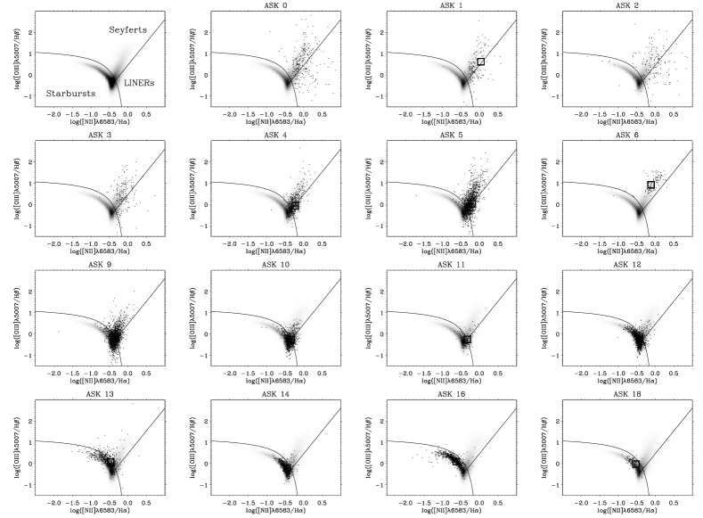
Figure 13.— BPT diagrams for the full set of galaxies with emission lines (top left panel), as well as for the galaxies belonging to the major ASK classes (remaining panels). The full set is shown as an image of the 2-dimensional histogram. This image is repeated in the rest of the panels for reference. We represent scatter plots for 10000 individual galaxies randomly drawn from the full SDSS/DR7 pool. The curved solid line separates star-forming galaxies (below the line) and AGNs (above the line). In addition, the straight solid line in the region of AGNs separates Seyfert galaxies and LINERs. The plots also include a box symbol for the class template spectrum when it contains the required emission lines. These boxes are often buried within the cloud of dots. Major classes 19 and 22 are not shown because they do not fit into the figure, but they follow the sequence.

Figure 13, top left panel, contains the BPT diagram for the full set of galaxies with emission lines. The fluxes of the lines have been directly taken from SDSS/DR7. The figure includes a curved solid line dividing star-forming galaxies (below the line) and AGNs (above the line). This separation was worked out by Kauffmann et al. (2003), where they also distinguish between different types of AGNs. The straight line separates the regions occupied by Seyfert galaxies, and LINERs, as indicated by the insets. The figure also shows BPT plots for the galaxies belonging to the individual ASK classes – see the class in the label on top of each plot. The panels for the classes include box symbols at the positions where class template spectra show up. They are barely visible because they always appear in the center of the cloud of points corresponding to the individual galaxies. (ASK 0, 2, and 3 do not have such boxes since they present H$\beta$ in absoption; see Table 2.)

Only a small fraction of red galaxies have emission lines that can be used to place them in the BPT diagram (2% for ASK  2; see Table 2), however, when they do, their emission corresponds to AGN activity (Fig. 13, ASK  0–2). This result is very much in agreement with the current views that host galaxies of AGNs are preferentially early type galaxies (Kauffmann et al. 2003, and references therein). Conversely, blue galaxies correspond to star-forming galaxies, with little sign (if any) of undergoing AGN activity (from ASK  9 on; see Fig. 13). The galaxies that seems to be in the green valley (ASK  3, ASK  5 and ASK  6; § 7), also appear in the BPT diagrams in the region of AGNs. This is again consistent with the current wisdom that AGN activity quenches star formation, and so it may be responsible for the transit of galaxies across the green valley (Schawinski et al. 2007, 2009) The case of ASK  6 deserves special attention. According to the position in the BPT diagram, there is little doubt that it is formed by Seyfert galaxies. This is consistent with the shape of H$\alpha$ in the class template spectrum, with very broad wings that extend up to 2000 km s^-1. Moreover the only galaxy in the catalog by Kennicutt (1992) classified as ASK  6 is a well known cD elliptical with a Seyfert nucleus (NGC 1275; see Fig. 11).

9. Relationship between ASK class and redshift

Cone diagrams (or pie plots) are polar plots where radius is redshift and azimuth is right ascension (e.g., Folkes et al. 1999). Figure 14 shows cone diagrams for four representative classes, i.e., a red galaxy class (ASK  2), an AGN class (ASK  6), and two blue galaxy classes (ASK  9 and ASK  16). The range of declinations is limited between $35^{\circ}$ and $45^{\circ}$.

Figure 14.— Cone diagrams of four representative classes: a red galaxy class (ASK  2), an AGN class (ASK  6), and two classes of blue galaxies (ASK  9 and ASK  16). Cone diagrams are polar plots where radius is redshift and azimuth is right ascension. In this case $35^{\circ}\leq$ declination $\leq 45^{\circ}$, and redshift $\leq 0.5$ (see the labels on the rings). We are representing only a small fraction of all galaxies to avoid cluttering.

From Fig. 14 and similar plots considering other classes, other range of redshifts, and other declinations, we draw the following conclusions. ASK 0, 1, 2, and 3 are observed at higher redshifts than the rest of the classes. This effect is partly due to the luminous red galaxy (LRG) extension of the main SDSS spectroscopic sample (Eisenstein et al. 2001). The LRG search has been designed to detect passively evolving red galaxies, and it includes galaxies fainter than the main flux-limited portion of the SDSS galaxy spectroscopic sample (down to $r\simeq$ 19.5, rather than the regular cutoff at $r\simeq$ 17.8). However, a part of the separation in redshift between blue galaxies and red galaxies is believed to be real. Dwarf galaxies cannot be observed at high redshift, but dwarf field galaxies tend to be starforming (e.g., Heavens et al. 2004), and so included among the bluest ASK classes. It is therefore understandable why blue ASK classes are biases towards lower redshifts. Proper motions induced by the large gravitational potential of galaxy clusters lead to the so-called fingers of god in the cone diagrams, i.e., elongated clumps with the major axis pointing toward the observer (e.g., Jackson 1972). We find them preferentially in ASK  2 cone diagrams, which we interpret as an inclination for the red galaxies to be in clusters. ASK  6 is formed by Seyfert galaxies, and it seems to be more spreadout than the other classes (see Fig. 14). Finally, we find not distinct or sharp change of properties at redshift 0.25, i.e., at the divide used to split the classification (see § 4). Galaxies at redshifts larger than this value were not used to derive the classes. The featureless transition at this special redshift indicates no obvious systematic difference between the galaxies that define the classes, and the rest.

10. Retrieving physical properties of individual galaxies by interpolation

One can foresee several applications of the classification, in particular, it can be used to derive non-trivial physical parameters of individual galaxies by interpolation of the properties of the classes. We want to measure the parameter $X$ for the galaxy ${\bf s}$. Assume that the parameter $X$ varies systematically along the ASK sequence, being $X_{i}$ in the $i$-th class. Then, one can approximate $X$ for galaxy s as,

$$X({\bf s})\simeq{\sum_{i=0}^{27}Q_{i}({\bf s})\,X_{i}}\Big{/}{\sum_{i=0}^{27}Q_{i}({\bf s})},$$ (13)

where $Q_{i}({\bf s})$ represent the qualities assigned to the galaxy as explained in § 2.3, except that we have shorten the notation so that,

$$Q_{i}({\bf s})=Q({\bf c_{i}},{\bf s},{\bf c_{k}}).$$ (14)

In practice, the series (13) can be truncated to consider only a few terms where the quality is large enough. Regardless of the complications to estimate a given parameter, by having the classification and the value of the physical parameter in the ASK classes, equation (13) trivially provides the parameter for all SDSS/DR7. We have used the Star Formation Rate (SFR) to illustrate the procedure (Fig. 15). The equivalent width of H$\alpha$ is a proxy for Specific SFR (or SSFR) (e.g. Kennicutt 1998), and it varies systematically along the ASK sequence (Table 2). Using the empirical relationship between H$\alpha$ flux and SFR as calibrated by Kennicutt (1998), Fig. 15 shows a scatter plot with the SFRs obtained directly and by interpolation based on equation (13). The figure considers only starforming galaxies, i.e., ASK  $\geq 7$ according to § 8. We truncate the series using only the three classes of highest qualities. Figure 15 shows that interpolated SFRs are correct within a factor of two for SFRs varying four orders of magnitude. Unfortunately, the interpolation does not work in all cases. We failed to estimate metallicities by interpolation. The oxygen metallicity has a large dispersion within each ASK class and, therefore, it does not meet the condition of varying systematically along the ASK sequence.

Figure 15.— Scatter plot of Star Formation Rates (SFRs) inferred by interpolation on the ASK classes (ordinates) versus SFR from the parameters of the individual galaxies (abscissas). The diagonal solid line indicates where abscissas and ordinates coincide. Only a subset of randomly selected starforming galaxies is represented (ASK  $\geq 7$).

The interpolation may be specially useful when dealing with high redshift objects for which only noisy spectra are available. Once each spectrum is assigned to a particular class, one can assign all the properties of the class to the spectrum. In this sense, one can use the spectra of the different classes as templates for redshift determinations (e.g., Le Fèvre et al. 2005; Lilly et al. 2007). They represent a unique set able to reproduce all kinds of local galaxies. Unfortunately, the available redshift range is limitted since the bluest wavelength of the templates is as red as 3800 Å, and galaxies with redshift $>2.5$ will not overlap in any wavelength with the templates. However, one could overcome this problem classifying galaxies at various redshift ranges in various steps, very much in the vein of the classification for galaxies with redshift $>0.25$ explained in § 4. After classification, the blue part of the average high redshift spectra can be used to provide blue parts for the templates. New templates with extended blue wavelengths would be available, which can be used to extend the range even further by repeating the previous step. One can also use the classification to carry out relative measurements. For example, even if we ignore the metallicity of a galaxy, one can infer whether it is metal rich or poor with respect to the class mates using simple tools like the ratio between the fluxes of [NII]$\lambda$6583 and H$\alpha$ (e.g., Pettini & Pagel 2004). All the systematic errors involved in such comparison would be greatly reduced within a class (e.g., Stasińska 2004; Sánchez Almeida et al. 2009). Moreover, if the absolute metallicity of the class template is known, these simple recipes for relative measurements yield absolute metallicities using the class spectrum for reference.

11. Discussion and conclusions

We present an automatic unsupervised classification of all the galaxies with spectra in the final SDSS data release (DR7). It uses the k-means algorithm, which separates the 930000 galaxies into 17 major classes containing 99% of the galaxies, plus another 11 minor classes with the rest. The algorithm guarantees that the galaxies in a class have similar spectra, independently of their luminosities. The algorithm does guarantees that the classes represent true clusters in the classification space, nor that all existing clusters are identified. Each ASK class is characterized by an extra-low noise spectrum resulting from averaging all the spectra in the class. These template spectra vary smoothly and systematically among the classes, labeled according to their $g-r$ color from ASK 0, the reddest, to ASK 27, the bluest (Fig. 4 and Table 2). The classes are well separated in the color sequence, with a class that collects most of the red sequence galaxies (ASK 2), a set of classes lying along the blue cloud (ASK 9 and larger), and a class that seems to be characteristic of the green valley (ASK 5); see § 7. Usually the classes of red galaxies do not present emission lines, however, when they do, their excitation is characteristic of AGN activity. In contrast, all the galaxies in the classes on the blue cloud seem to present emission lines, but they are typical of star formation regions. The classes in between (i.e., in the green valley) show AGN activity (see § 8). The ASK classification has been compared with the morphological Hubble type. Although the number of galaxies involved in this comparison is rather limited, it clearly shows how the red classes tend to have early morphological types, whereas the blue classes are morphologically late types (Fig. 11 and § 6). The relationship has a large intrinsic scatter, as previous studies also find (see § 1.1). We have confronted the ASK classes with the PCA-based spectroscopic classification also existing for SDSS/DR7 (§ 5). The two of them are consistent in the sense that ASK classes have well defined PCA eigenvalues. However, the ASK classes are finer. We note that the scatter between these two purely spectroscopic classifications is much smaller than the scatter in the relationship with Hubble type (§ 6). The distribution of classes with redshifts is studied in § 9, and it reveals that the bluer classes contain galaxies of lower redshift, indicating that they are made of galaxies less luminous (and so smaller) than the red classes. The same preliminary analysis also suggests a trend for the red classes to be more clustered than the blue classes.

All the above properties prove the consistency of the ASK classification. We have not found obvious contradictions between the physical properties of the classes, and the present understanding of galaxy properties. However, one should not forget the limitations of the analysis. The classification is not unique. We know that the borders between classes are not well defined, and that the actual number of classes is somewhat arbitrary (§ 4; § 2.1). The galaxy spectra seem to have a continuous distribution of properties, and we still ignore the reasons why k-means puts the borders between classes where it does. Moreover, the classification rely on a number of reasonable but otherwise subjective hypotheses (e.g., the spectral bandpasses entering into the classification, or the normalization to the g-band; see § 3 and Table 1). Alternative hypotheses would render classifications differing from ASK in a way difficult to foretell. All these caveats notwithstanding, the classes inferred by ASK have different spectra that reflect a systematic difference in the gas and stars present in the galaxies. Understanding the physical reasons causing the systematic differences between spectra would help understanding the classification itself. The study of the physical causes responsible for the observed diversity represents a major task that clearly goes beyond the scope of our introductory paper. However, a number of follow-up works dealing with the physical interpretation of classes are underway. As a result, some of the classes may need to be joined or split. For example, spectra of similar objects with different degrees of extinction may have ended up in different classes (remember that we do not correct for extinction to attain a purely empirical classification; § 3). Similarly, some of the classes may contain unidentified clusters. Sub-divisions can be achieved by applying k-means to selected spectral windows (e.g., the region around H$\alpha$ may help us separating emission line galaxies according to their metallicity; Pettini & Pagel 2004). Deriving the star formation history of the classes is fundamental to understand whether the differences between spectra are tracing different star formation histories, AGN activities, merging histories, or something else. (Is the ASK classification revealing some sort of evolutive sequence for galaxies?) Fortunately, inversion codes able to constrain the star formation history are available (e.g., Cid Fernandes et al. 2005; Tojeiro et al. 2009), and we plan to use them. We are also carrying out a comparison between morphological types and spectroscopic types in a way that completes the introductory exercise in § 6. We try to understand what causes the scatter in the relationship between morphology and spectroscopy. Is it the different characteristic time of evolution of morphological changes (on short timescales) and spectroscopic changes (on long timescales)? Is it the environment? The morphological classification will be based on the automatic procedure by Huertas-Company et al. (2008) using support vector machines, which will allow us to afford comparing morphology and spectral type for a sizeable fraction of the SDSS/DR7 spectroscopic catalog. Work to derive the luminosity function for the classes is pending, i.e., to characterize the number density of galaxies of each luminosity and class. It is needed to quantify the tendency for high ASK classes to contain dwarf galaxies, as suggested in § 9.

In addition to understanding the physical mechanisms responsible for the diversity among spectra, we foresee other applications of the ASK classification. It provides a crude but fast way of estimating some physical properties of a galaxy once its ASK ascription is known (§ 10). The classification is also useful as target selection. For example, ASK 6 is formed by Seyfert galaxies. This class provides an ideal homogeneous sample of some 5000 Seyferts with similar spectra for in-depth AGN studies (e.g., extending to low mass the relationship between supermassive black-hole mass and bulge mass; see Ferrarese 2006, and references therein). The classification supplies classes of galaxies in the green valley (ASK 5). These targets allow us addressing the question of what characterizes a green valley galaxy, and one can do it in a statistically significant way. Is the green valley a short period during the life of any galaxy, or does it represent a genuine class of galaxies separated from the rest? The qualities assigned to each galaxy provide a simple way to find unusual objects. Low quality galaxies are outliers of the classification and, therefore, abnormal objects that deserve specific follow-up work. The average spectra of the classes can be used as template for redshift determinations. They represent a unique set comprising all spectral types. This application of ASK requires extending the template spectra to the UV, but this upgrade can be done in successive steps as outlined in § 10.

In order to facilitate these and possibly other applications, we have made the ASK classification freely available though the ftpsite ftp://ask:galaxy@ftp.iac.es/. We explain how it can be directly employed in SQL queries that use the CasJob facility of SDSS/DR7. We also provide it as ASCII csv tables suitable for uses external to SDSS. In addition, the template spectra are included.

Acknowledgments. We are indebted to J. Betancort, I. G. de la Rosa, and M. Moles, that contributed with discusions on their area of expertise. Thanks to an anonymous referee we include the discussion on the degree of clustering of the classes at the end of § 4. The work has been partly funded by the Spanish Ministries of science, technology and innovation, projects AYA 2007-67965-03-1, AYA 2007-67752-C03-01, and CSD2006-00070. Funding for the Sloan Digital Sky Survey (SDSS) and SDSS-II has been provided by the Alfred P. Sloan Foundation, the Participating Institutions, the National Science Foundation, the U.S. Department of Energy, the National Aeronautics and Space Administration, the Japanese Monbukagakusho, and the Max Planck Society, and the Higher Education Funding Council for England. The SDSS is managed by the Astrophysical Research Consortium (ARC) for the Participating Institutions. The Participating Institutions are the American Museum of Natural History, Astrophysical Institute Potsdam, University of Basel, University of Cambridge, Case Western Reserve University, The University of Chicago, Drexel University, Fermilab, the Institute for Advanced Study, the Japan Participation Group, The Johns Hopkins University, the Joint Institute for Nuclear Astrophysics, the Kavli Institute for Particle Astrophysics and Cosmology, the Korean Scientist Group, the Chinese Academy of Sciences (LAMOST), Los Alamos National Laboratory, the Max-Planck-Institute for Astronomy (MPIA), the Max-Planck-Institute for Astrophysics (MPA), New Mexico State University, Ohio State University, University of Pittsburgh, University of Portsmouth, Princeton University, the United States Naval Observatory, and the University of Washington.

Appendix A Galaxies in a cluster as a function of the cluster center

The random initialization of k-means leads to small uncertainties in the properties of the clusters which, however, produce a significant variation on the actual galaxies assigned to each cluster (§ 2, § 4). This amplification can be understood by considering that clusters are defined by regions in a space of many dimensions. A small uncertainty in the center of the cluster produces large (relative) variations of the region of space that the cluster samples. Below we compute this boost factor under the simplifying assumption that the clusters are defined by hyper-spheres. Such simplification should not affect the conclusion we draw since the scaling relationship between volume and area is a general property of the space, rather then specific to a particular shape.

Assume that the galaxies belonging to a class are those within a sphere of radius $R$ centered in the class center. Assume that the galaxies are uniformly distributed around this center. Two different runs of the k-means clustering algorithm yield slightly different centers for the class, separated by a distance $\Delta R$. How many galaxies will be shared by the two classifications? Under the previous hypotheses, it is just the overlapping volume of two $n-$dimensional hyper-spheres of radius $R$ when their centers are separated $\Delta R$. When $\Delta R/R\ll 1$, such volume is the volume of one of the original hyper-spheres minus the volume of a cylinder of height $\Delta R$ and base the corresponding $n-$dimensional hyper-disk (i.e., an hyper-sphere in $n-1$ dimensions). Using the expression for the volume of a sphere in $n$ dimensions, the number of common galaxies, $N(\Delta R)$, normalized to the number of galaxies in the class, $N(0)$, turns out to be,

$${{N(\Delta R)}\over{N(0)}}\simeq 1-{{\Delta R}\over{R}}\sqrt{n/2\pi}.$$ (A1)

Equation (A1) shows how a small relative error in the position of the cluster center gets amplified as $\sqrt{n/2\pi}$ when affecting the drop in the number of common galaxies. Since $n\gg 1$, the drop is very large. For example, if $n=2000$, a minute $\Delta R/R\simeq 2$% produces $N(\Delta R)/N(0)\simeq$ 65%. Variations induced by cluster radius changes are even more dramatic. In this case the boost factor scales with $n$ rather than $\sqrt{n}$.

References

- Aaronson (1978) Aaronson, M. 1978, ApJ, 221, L103
- Abazajian et al. (2009) Abazajian, K. N., Adelman-McCarthy, J. K., Agüeros, M. A., et al. 2009, ApJS, 182, 543
- Baldry et al. (2004) Baldry, I. K., Glazebrook, K., Brinkmann, J., et al. 2004, ApJ, 600, 681
- Baldwin et al. (1981) Baldwin, J. A., Phillips, M. M., & Terlevich, R. 1981, PASP, 93, 5
- Balogh et al. (2004) Balogh, M. L., Baldry, I. K., Nichol, R., et al. 2004, ApJ, 615, L101
- Bershady (1995) Bershady, M. A. 1995, AJ, 109, 87
- Bershady et al. (2000) Bershady, M. A., Jangren, A., & Conselice, C. J. 2000, AJ, 119, 2645
- Bishop (2006) Bishop, C. M. 2006, Pattern Recognition and Machine Learning (NY: Springer)
- Blanton & Roweis (2007) Blanton, M. R. & Roweis, S. 2007, AJ, 133, 734
- Bradley & Fayyad (1998) Bradley, P. S. & Fayyad, U. M. 1998, Refining Initial Points for k-means Clustering, Tech. rep., Microsoft Research, MSR-TR-98-36
- Bromley et al. (1998) Bromley, B. C., Press, W. H., Lin, H., & Kirshner, R. P. 1998, ApJ, 505, 25
- Chan et al. (2003) Chan, B. H. P., Mitchell, D. A., & Cram, L. E. 2003, MNRAS, 338, 790
- Cid Fernandes et al. (2005) Cid Fernandes, R., Mateus, A., Sodré, L., Stasińska, G., & Gomes, J. M. 2005, MNRAS, 358, 363
- Connolly et al. (1995) Connolly, A. J., Szalay, A. S., Bershady, M. A., Kinney, A. L., & Calzetti, D. 1995, AJ, 110, 1071
- Conselice (2006) Conselice, C. J. 2006, MNRAS, 373, 1389
- Deeming (1964) Deeming, T. J. 1964, MNRAS, 127, 493
- Eisenstein et al. (2001) Eisenstein, D. J., Annis, J., Gunn, J. E., et al. 2001, AJ, 122, 2267
- Everitt (1995) Everitt, B. S. 1995, Cluster Analysis (London: Arnold)
- Ferrarese (2006) Ferrarese, L. 2006, in Joint Evolution of Black Holes and Galaxies, ed. M. Colpi, V. Gorini, F. Haardt, & U. Moschella (New York: Taylor & Francis), 1
- Ferreras et al. (2006) Ferreras, I., Pasquali, A., de Carvalho, R. R., de la Rosa, I. G., & Lahav, O. 2006, MNRAS, 370, 828
- Folkes et al. (1999) Folkes, S., Ronen, S., Price, I., et al. 1999, MNRAS, 308, 459
- Folkes et al. (1996) Folkes, S. R., Lahav, O., & Maddox, S. J. 1996, MNRAS, 283, 651
- Formiggini & Brosch (2004) Formiggini, L. & Brosch, N. 2004, MNRAS, 350, 1067
- Francis et al. (1992) Francis, P. J., Hewett, P. C., Foltz, C. B., & Chaffee, F. H. 1992, ApJ, 398, 476
- Fukugita et al. (2007) Fukugita, M., Nakamura, O., Okamura, S., et al. 2007, AJ, 134, 579
- Heavens et al. (2004) Heavens, A., Panter, B., Jimenez, R., & Dunlop, J. 2004, Nature, 428, 625
- Hubble (1936) Hubble, E. P. 1936, Realm of the Nebulae (New Haven: Yale University Press)
- Huertas-Company et al. (2008) Huertas-Company, M., Rouan, D., Tasca, L., Soucail, G., & Le Fèvre, O. 2008, A&A, 478, 971
- Huertas-Company et. al. (2009) Huertas-Company et. al., M. 2009, A&A, submitted
- Humason (1931) Humason, M. L. 1931, ApJ, 74, 35
- Jackson (1972) Jackson, J. C. 1972, MNRAS, 156, 1P
- Kannappan et al. (2009) Kannappan, S. J., Guie, J. M., & Baker, A. J. 2009, AJ, 138, 579
- Kauffmann et al. (2003) Kauffmann, G., Heckman, T. M., Tremonti, C., et al. 2003, MNRAS, 346, 1055
- Kennicutt (1998) Kennicutt, Jr., R. C. 1998, ARA&A, 36, 189
- Kennicutt (1992) Kennicutt, Jr., R. C. 1992, ApJS, 79, 255
- Le Fèvre et al. (2005) Le Fèvre, O., Vettolani, G., Garilli, B., et al. 2005, A&A, 439, 845
- Lilly et al. (2007) Lilly, S. J., Le Fèvre, O., Renzini, A., et al. 2007, ApJS, 172, 70
- Lu et al. (2006) Lu, H., Zhou, H., Wang, J., et al. 2006, AJ, 131, 790
- Madgwick (2003) Madgwick, D. S. 2003, MNRAS, 338, 197
- Madgwick et al. (2003) Madgwick, D. S., Coil, A. L., Conselice, C. J., et al. 2003, ApJ, 599, 997
- Mittaz et al. (1990) Mittaz, J. P. D., Penston, M. V., & Snijders, M. A. J. 1990, MNRAS, 242, 370
- Morgan & Mayall (1957) Morgan, W. W. & Mayall, N. U. 1957, PASP, 69, 291
- Peña et al. (1999) Peña, J. M., Lozano, J. A., & Larrañaga, P. 1999, Pattern Recognition Letters, 20, 1027
- Pettini & Pagel (2004) Pettini, M. & Pagel, B. E. J. 2004, MNRAS, 348, L59
- Reichardt et al. (2001) Reichardt, C., Jimenez, R., & Heavens, A. F. 2001, MNRAS, 327, 849
- Salim et al. (2007) Salim, S., Rich, R. M., Charlot, S., et al. 2007, ApJS, 173, 267
- Sánchez Almeida et al. (2009) Sánchez Almeida, J., Aguerri, J. A., Muñoz-Tuñón, C., & Vazdekis, A. 2009, ApJ, 698, 1497
- Sánchez Almeida & Lites (2000) Sánchez Almeida, J. & Lites, B. W. 2000, ApJ, 532, 1215
- Sandage (2005) Sandage, A. 2005, ARA&A, 43, 581
- Schawinski et al. (2009) Schawinski, K., Lintott, C. J., Thomas, D., et al. 2009, ApJ, 690, 1672
- Schawinski et al. (2007) Schawinski, K., Thomas, D., Sarzi, M., et al. 2007, MNRAS, 382, 1415
- Slonim et al. (2001) Slonim, N., Somerville, R., Tishby, N., & Lahav, O. 2001, MNRAS, 323, 270
- Sodre & Cuevas (1997) Sodre, L. & Cuevas, H. 1997, MNRAS, 287, 137
- Sodré & Cuevas (1994) Sodré, Jr., L. & Cuevas, H. 1994, Vistas in Astronomy, 38, 287
- Stasińska (2004) Stasińska, G. 2004, in Cosmochemistry. The melting pot of the elements, ed. C. Esteban, R. García López, A. Herrero, & F. Sánchez (Cambridge: CUP), 115
- Stoughton et al. (2002) Stoughton, C., Lupton, R. H., Bernardi, M., et al. 2002, AJ, 123, 485
- Strateva et al. (2001) Strateva, I., Ivezić, Ž., Knapp, G. R., et al. 2001, AJ, 122, 1861
- Tojeiro et al. (2009) Tojeiro, R., Wilkins, S., Heavens, A. F., Panter, B., & Jimenez, R. 2009, ApJS, 185, 1
- Vanderplas & Connolly (2009) Vanderplas, J. & Connolly, A. 2009, AJ, 138, 1365
- Whitney (1983) Whitney, C. A. 1983, A&AS, 51, 443
- Worthey et al. (1994) Worthey, G., Faber, S. M., Gonzalez, J. J., & Burstein, D. 1994, ApJS, 94, 687
- Worthey & Ottaviani (1997) Worthey, G. & Ottaviani, D. L. 1997, ApJS, 111, 377
- Yip et al. (2004) Yip, C. W., Connolly, A. J., Szalay, A. S., et al. 2004, AJ, 128, 585
- Zaritsky et al. (1995) Zaritsky, D., Zabludoff, A. I., & Willick, J. A. 1995, AJ, 110, 1602