Spectral function of the Anderson impurity model at finite temperatures

Abstract

Using the functional renormalization group (FRG) and the numerical renormalization group (NRG), we calculate the spectral function of the Anderson impurity model at zero and finite temperatures. In our FRG scheme spin fluctuations are treated non-perturbatively via a suitable Hubbard-Stratonovich field, but vertex corrections are neglected. A comparison with our highly accurate NRG results shows that this FRG scheme gives a quantitatively good description of the spectral line-shape at zero and finite temperatures both in the weak and strong coupling regimes, although at zero temperature the FRG is not able to reproduce the known exponential narrowing of the Kondo resonance at strong coupling.

I Introduction

In the past decade, the experimental realization of man-made nanostructures such as quantum dots coupled to a metallic environmentGoldhaber98 ; Cronenwett98 has brought renewed attention to the theoretical handling of the Anderson impurity model (AIM). Moreover, the solution of the AIM represents one of the fundamental steps in the so-called dynamical mean-field theory, Georges96 describing the quantum dynamics of the Hubbard model in the limit of infinite spatial dimensions, Metzner89 where the effects of the dynamical Weiss field can be described in terms of an effective local impurity model subject to a self-consistency condition. Because the thermodynamics of the AIM can be obtained exactly by means of the Bethe Ansatz Tsvelick83 ; Hewson93 and, on the other hand, Wilson’s numerical renormalization group Wilson75 (NRG) gives a numerically controlled method of calculating spectral properties, Costi94 ; Hofstetter00 ; Peters06 ; Weichselbaum07 ; Bulla08 the AIM can also be used as a benchmark model for testing various non-perturbative many-body methods. It is therefore important to develop reliable methods for solving the AIM especially at intermediate and strong coupling which require low computational effort, in the perspective of tackling the more complex impurity problems arising from both dynamical mean-field theory applications and experimental realizations of nanostructure devices.

Motivated by the above considerations, several authors have tried to reproduce at least some aspects of the known properties of the AIM using functional renormalization group (FRG) methods. Hedden04 ; Karrasch08 ; Bartosch09 ; Jakobs09 Although the FRG gives a formally exact hierarchy of integro-differential equations for all irreducible vertices, Berges02 ; Pawlowski07 ; Kopietz10 ; Rosten10 in practice this hierarchy has to be truncated in order to extract physical information from it. Unfortunately, at this point no truncation of this hierarchy has been found which correctly reproduces all the known strong-coupling properties of the AIM, such as the correct interaction dependence of the Kondo scale, which is known to be exponentially small in the interaction strength. In fact, the proper construction of unbiased truncations of the formally exact FRG flow equations which do not break down in the strong coupling limit is a largely unsolved problem in the field.

Quite generally, some progress in solving the FRG flow equations can be made if the dominant fluctuation channel is known a priori. For example, for the description of superfluidity in the attractive Fermi gas the particle-particle channel is known to play a special role. In such a situation it is natural to decouple the interaction in the particle-particle channel using a Hubbard-Stratonovich transformation and consider the FRG flow of the coupled mixed fermion-boson model. Kopietz10 ; Bartosch09b ; Schuetz05 ; Floerchinger08b ; Strack08 ; Diehl09

In Ref. [Bartosch09, ] a similar strategy has been applied to the AIM, although in this case the proper choice of the Hubbard-Stratonovich decoupling is not so obvious. For simplicity, we shall focus in this work on the local moment regime of the symmetric AIM at intermediate to strong coupling; in this case the physics is dominated by spin fluctuations, so that one should decouple the on-site interaction in the spin-fluctuation channels. Still, the decoupling is ambiguous because of the freedom of distributing the interaction between transverse and longitudinal spin channels. In the simplest case, the decoupling is then performed such that only transverse spin-fluctuations are explicitly introduced. The resulting FRG flow equations have already been derived in Ref. [Bartosch09, ], but further approximations have been made to reduce the resulting integro-differential equation to an ordinary differential equation for the wave-function renormalization factor $Z$. Unfortunately, in this approximation only the low-energy features of the spectral function can be described. In this work we shall not rely on such a low-energy approximation, but present a fully self-consistent solution of the integro-differential equation for the self-energy of the AIM. This enables us to calculate the full spectral line-shape of the AIM at all energy scales. In order to test the accuracy of our FRG approach, we shall also calculate the spectral function at zero and finite temperatures using the highly reliable NRG approach. By comparing the results obtained with the two methods, we then show that our rather simple truncation of the FRG flow equations gives a quantitatively accurate description of the spectral function of the AIM at all energies.

II FRG with partial bosonization in the spin singlet channel

The AIM describes a single localized electron level which is coupled to a band of non-interacting conduction electrons. The latter degrees of freedom can be integrated out so that the partition function can be written as a fermionic functional integral involving only Grassmann fields $d_{\sigma}(\tau)$ and $\bar{d}_{\sigma}(\tau)$ associated with the localized electrons. Here $\sigma=\uparrow,\downarrow$ labels the spin projection, and $\tau$ is the imaginary time. Following Ref. [Bartosch09, ] we decouple the local on-site interaction by means of a complex bosonic Hubbard-Stratonovich field $\chi$ in the spin-singlet particle-hole channel. The partition function $\cal{Z}$ divided by the corresponding partition function $\cal{Z}_{\rm HF}$ in Hartree-Fock approximation can then be written as

$$\frac{\cal{Z}}{{\cal{Z}}_{\rm HF}}=\frac{\int{\cal{D}}[\bar{d},d,\bar{\chi},\chi]e^{-S_{0}[\bar{d},d,\bar{\chi},\chi]-S_{1}[\bar{d},d,\bar{\chi},\chi]}}{\int{\cal{D}}[\bar{d},d,\bar{\chi},\chi]e^{-S_{0}[\bar{d},d,\bar{\chi},\chi]}}.$$ (1)

The Gaussian part of the bare action is

$$S_{0}[\bar{d},d,\bar{\chi},\chi] = -\int_{\omega}\sum_{\sigma}{G}_{0}^{-1}(i\omega)\bar{d}_{\omega\sigma}{d}_{\omega\sigma}$$ (2)

$$+\int_{\bar{\omega}}U^{-1}\bar{\chi}_{\bar{\omega}}\chi_{\bar{\omega}},$$

while the interaction part can be written as

$$S_{1}[\bar{d},d,\bar{\chi},\chi]=\int_{\bar{\omega}}\int_{\omega}\left[\bar{d}_{\omega+\bar{\omega}\uparrow}d_{\omega\downarrow}{\chi}_{\bar{\omega}}+\bar{d}_{\omega\downarrow}d_{\omega+\bar{\omega}\uparrow}\bar{\chi}_{\bar{\omega}}\right],$$ (3)

where $\int_{\omega}=\beta^{-1}\sum_{\omega}$ denotes summation over fermionic Matsubara frequencies $i\omega$, with $\beta=1/T$ being the inverse temperature, whereas $\int_{\bar{\omega}}=\beta^{-1}\sum_{\bar{\omega}}$ denotes summation over bosonic Matsubara frequencies $i\bar{\omega}$ (in the zero temperature limit the sums are replaced by integrals). For simplicity we consider only the symmetric AIM in the wide band limit, where the Hartree-Fock propagator is given by

$$G_{0}(i\omega)=\frac{1}{i\omega+i\Delta{\,\rm sign\,}\omega}.$$ (4)

In the above expression the energy scale $\Delta$ arises from the hybridization between the localized $d$-electrons, represented by the Grassmann variables $d_{\sigma}$ and $\bar{d}_{\sigma}$, and the conduction electrons. The exact $d$-electron propagator, on the other hand, is of the form

$$G(i\omega)=\frac{1}{i\omega+i\Delta{\,\rm sign\,}\omega-\Sigma(i\omega)}.$$ (5)

Our aim is to calculate the irreducible self-energy $\Sigma(i\omega)$ using the FRG and then analytically continue it to the real frequency axis.

We use here the frequency transfer cutoff scheme proposed in Ref. [Bartosch09, ], where an infrared cutoff is introduced only into the bosonic part of the Gaussian action (2). Specifically, we introduce the cutoff via the following substitution in the second line of Eq. (2),

$$U^{-1}\rightarrow U^{-1}+R_{\Lambda}(i\bar{\omega}),$$ (6)

where

$$R_{\Lambda}(i\bar{\omega})=\frac{\Lambda}{\pi\Delta^{2}}R(|\bar{\omega}|/\Lambda),$$ (7)

and the function $R(x)$ is defined byLitim01

$$R(x)=(1-x)\Theta(1-x).$$ (8)

Our implementation of the FRG method is therefore different from previous purely fermionic FRG studies of the AIM, Hedden04 ; Karrasch08 where no Hubbard-Stratonovich fields were introduced. The advantages of our scheme are that the resulting FRG flow equations can be analyzed with moderate numerical effort and yield a quantitatively accurate description of both the low-energy and high-energy features (such as the broadened Hubbard peaks) of the spectral function. Neglecting vertex corrections, the FRG flow of the cutoff-dependent self-energy reads

$$\partial_{\Lambda}\Sigma_{\Lambda}(i\omega) = \int_{\bar{\omega}}\dot{F}_{\Lambda}(i\bar{\omega})G_{\Lambda}(i\omega-i\bar{\omega}),$$ (9)

where the flowing fermionic propagator $G_{\Lambda}(i\omega)$ depends again on the flowing self-energy,

$$G_{\Lambda}(i\omega)=\frac{1}{i\omega+i\Delta{\,\rm sign\,}\omega-\Sigma_{\Lambda}(i\omega)},$$ (10)

and the bosonic single-scale propagator is given by

$$\dot{F}_{\Lambda}(i\bar{\omega})=[-\partial_{\Lambda}R_{\Lambda}(i\bar{\omega})][F_{\Lambda}(i\bar{\omega})]^{2},$$ (11)

with the bosonic propagator given by

$$F_{\Lambda}(i\bar{\omega}) = \frac{1}{U^{-1}+R_{\Lambda}(i\bar{\omega})-\Pi_{\Lambda}(i\bar{\omega})}.$$ (12)

Here, $\Pi_{\Lambda}(i\bar{\omega})$ represents the flowing irreducible spin susceptibility, which can be related to the fermionic Green function, in the absence of vertex corrections, by means of the following (skeleton) equation, Bartosch09

$$\Pi_{\Lambda}(i\bar{\omega}) = -\int_{\omega}G_{\Lambda}(i\omega)G_{\Lambda}(i\omega-i\bar{\omega})\;.$$ (13)

Substituting Eqs. (10)–(13) into Eq. (9) we obtain a closed integro-differential equation for the flowing self-energy $\Sigma_{\Lambda}(i\omega)$, which must be integrated from the initial scale $\Lambda_{0}\to\infty$, with initial condition $\Sigma_{\Lambda_{0}}(i\omega)\equiv 0$, down to $\Lambda=0$. The physical self-energy is then given by the limit $\Sigma(i\omega)=\lim_{\Lambda\to 0}\Sigma_{\Lambda}(i\omega)$.

Before discussing the details of our numerical approach to Eq. (9), it is worthwhile to remark that in Ref. [Bartosch09, ] the corresponding flow equation for $\Sigma_{\Lambda}(i\omega)$ was treated in a very crude approximation, namely by expanding all quantities appearing in Eq. (9) to linear order in frequency. As a consequence, only the low-energy properties of the spectrum, characterized by the $\omega=0$ quasiparticle peak, were accessible. Moreover, the results were obtained only in the zero-temperature limit. Here, on the other hand, we do not rely on any low-energy expansion, so that we can calculate the spectral function at all energy scales and describe the transfer of spectral weight, in the strong-coupling regime, from the Kondo peak to the high-energy Hubbard bands.

III Numerical solution of the FRG equation for the self-energy

III.1 Zero temperature

In the zero temperature limit all the sums over Matsubara frequencies are replaced by integrals, $\beta^{-1}\sum_{\omega}\to\int\frac{d\omega}{2\pi}$. The flow equation for $\Sigma_{\Lambda}(i\omega)$ reduces therefore to an integro-differential equation, which requires an artificial discretization of the imaginary axis in order to be solved numerically. More precisely, our numerical approach to Eq. (9) consists in replacing the flowing self-energy $\Sigma_{\Lambda}(i\omega)$, defined as a function of the continuous parameter $\omega$, by a finite set of flowing couplings $\Sigma_{\Lambda}(i\omega_{n})$ defined on a discrete mesh of frequencies $\omega_{n}$.

The choice of a specific parametrization of the Matsubara axis, at zero temperature, is in principle arbitrary; however, one has to carefully verify that the numerical results are actually independent of such a parametrization. In other words, the results should be numerically stable with respect to the choice of the discretization procedure. To achieve this goal we consider the following geometric meshKarrasch08 of frequencies,

$$\omega_{n}=\omega_{\rm min}\frac{a^{n}-1}{a-1},\qquad n=1,\ldots,N,$$ (14)

where the free parameters $a>1$ and $\omega_{\rm min}>0$ define the spacing of the frequencies, while $N$ is the total number of frequencies to be used (note that in the particle-hole symmetric case we have $\Sigma_{\Lambda}(i\omega)=-\Sigma_{\Lambda}(-i\omega)$, so that we do not need independent couplings for the negative frequencies). As thoroughly discussed in Ref. [Karrasch08, ], the unequal spacing of such a mesh allows indeed to resolve with great accuracy the low-energy regime of the spectrum, which is known to exhibit the sharp Kondo resonance at $\omega=0$, while covering, at the same time, a sufficiently wide range of frequencies in order to rule out the spurious effects of a finite frequency cutoff $\omega_{\rm max}=\omega_{N}$. More specifically, one has to simultaneously satisfy, for all the values of $U$ under consideration, the following conditions,

$$\omega_{\rm min} \ll Z(U)\Delta,$$ (15)

$$\omega_{\rm max} \gg \max(\Delta,U),$$ (16)

where

$$Z(U)=\left(1-\left.\frac{\partial\Sigma(i\omega)}{\partial(i\omega)}\right|_{\omega=0}\right)^{-1}$$ (17)

is the quasiparticle residue (proportional to the width of the Kondo peak), and afterwards verify that the results are numerically stable upon a further increase in both the spanned frequency range $[\omega_{\rm min},\omega_{\rm max}]$ and the number $N$ of sampling frequencies. A typical choice of the discretization parameters is, e.g.,

$$\omega_{\rm min}=10^{-6}\Delta,\quad a=1.06,\quad N=400,$$ (18)

which allows to solve the flow equations with a relatively small computational effort up to the strong-coupling regime $U\lesssim 8\pi\Delta$.

The resulting system of $N$ coupled differential equations for the flowing couplings $\Sigma_{\Lambda}(i\omega_{n})$ is solved by means of refined Runge-Kutta routines, using a linear interpolation procedure in order to evaluate the Green function in Eqs. (9) and (13) at frequencies that do not belong to the geometric mesh (i.e., when $\omega_{\ell}-\bar{\omega}_{\ell^{\prime}}\notin\{\omega_{n}\}$).

III.2 Finite temperatures

At finite temperatures the Matsubara space is intrinsically discrete, with fermionic and bosonic frequencies given by

$$\omega_{n}=(2n+1)\pi/\beta,\qquad\bar{\omega}_{n}=2n\pi/\beta,$$ (19)

so that the flowing self-energy itself is already defined as a countable set of couplings $\Sigma_{\Lambda}(i\omega_{n})$. Eq. (9) is therefore no longer a proper integro-differential equation, as in the zero temperature limit, but consists rather of an infinite set of coupled ordinary differential equations, which can be solved numerically by keeping only the first $N$ Matsubara frequencies.

In contrast to the zero temperature case, it is crucial to observe that now the spacing between consecutive points of the mesh is constant, its value $\delta\omega=2\pi T$ being dictated by the actual value of the temperature $T$. This fact simplifies the implementation of the numerical routines, since there is no need for any interpolating procedure; on the other hand, however, it limits the possibility of studying arbitrarily small temperatures. In fact, in order to obtain numerically stable results using the natural Matsubara discretization defined in Eq. (19), one typically needs $N\gtrsim 10^{3}$ for temperatures $T/\Delta\lesssim 0.1$, which already corresponds to a remarkable computational effort. In other words, although smaller values of $T/\Delta$ are still accessible from the numerical point of view, the computational time required becomes comparable to that of fully numerical methods (e.g. the NRG), making the present method numerically unworthy.

III.3 Analytical continuation

The solution of our flow equation gives, by construction, the physical self-energy along the imaginary axis, $\Sigma(i\omega)=\Sigma_{\Lambda=0}(i\omega)$. In order to access real frequency properties, such as the spectral function

$$A(\omega)=-\frac{1}{\pi}{\rm Im\,}G(i\omega\to\omega+i0),$$ (20)

we need to analytically continue our results for either $G(i\omega)$ or $\Sigma(i\omega)$ onto the real frequency axis. Since our numerical solutions are not affected by statistical errors, we perform the analytical continuation using the Padé approximation, Pade77 which we found to give more stable results if directly applied to the self-energy. In other words, we first evaluate the real frequency self-energy, $\Sigma(\omega)=\Sigma(i\omega\to\omega+i0)$, and afterwards calculate the corresponding Green function using the Dyson equation. The frequency dependence of the self-energy is indeed much more sensitive to the interaction-induced features of the model than the Green function itself, whose non-trivial behavior is masked by the asymptotic form of the non-interacting propagator.

IV Numerical Renormalization Group at Finite Temperatures

The numerical renormalization group method Wilson75 was first applied to the Anderson impurity model Krishna-murthy80 shortly after its introduction in 1975. Originally designed to calculate thermodynamic quantities at very low temperatures, the NRG has been extended over the last two decades to calculate more complex observables, such as the single particle spectral function investigated here (for a recent review covering many extensions and applications of the NRG, see Ref. [Bulla08, ]). We briefly mention several crucial developments which lead to improving the accuracy of dynamical correlation functions calculated by NRG: the $z$-trick averaging Yoshida90 which improves the resolution at frequencies close to the conduction-band edge; the introduction of the reduced density matrix Hofstetter00 in order to account for the correct low-temperature state when calculating the spectrum at higher frequencies; and finally, a recently developed smart choice of the basis for the full NRG Fock space, Anders05 which was designed to calculate the real-time evolution after a quantum quench, and successively has been applied to improve the accuracy of spectral functions for the single impurity Anderson model Peters06 by avoiding overcounting of spectral transitions within the NRG.

The NRG data presented here were obtained by the full density matrix approach, Weichselbaum07 which gives access to reliable finite-temperature spectra for frequencies as low as $\omega\approx T/5$. In combination with the self-energy trick Bulla98 and an average over $N_{z}=32$ slightly different discretizations of the conduction band Yoshida90 we obtain high-quality NRG spectra, which serve as a benchmark for the newly developed FRG scheme discussed above. A detailed description of the NRG method is beyond the scope of this publication; for details we refer the interested reader to Ref. [Weichselbaum07, ] and references therein.

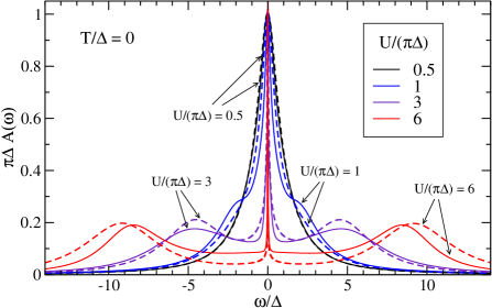
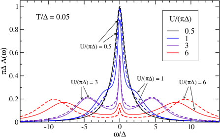
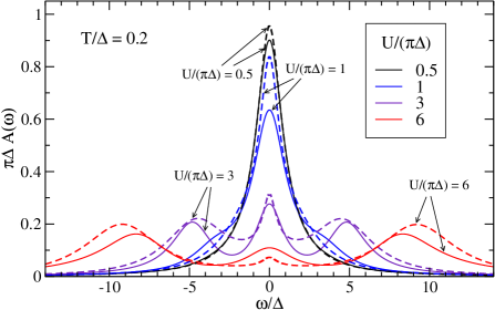
Figure 1: (Color online) Spectral function of the symmetric AIM evaluated with the FRG (solid lines) and the NRG (dashed lines) for different interactions and temperatures. From top to bottom the temperature increases from $T/\Delta=0$ to $T/\Delta=0.2$, as indicated.

V Results

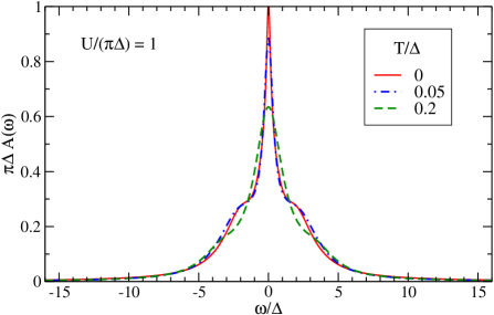
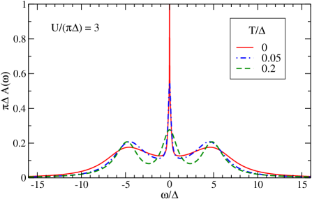
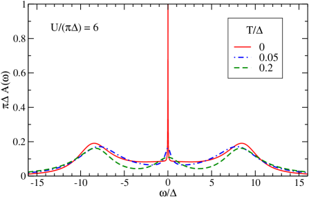
Figure 2: (Color online) FRG spectral function for different interactions and temperatures. From top to bottom the interaction increases from $U/(\pi\Delta)=1$ to $U/(\pi\Delta)=6$, as indicated.

Our results for the spectral function at temperatures $T/\Delta=0$, 0.05 and 0.2 are plotted in Fig. 1, where in each panel we have considered several values of the interaction strength, ranging from the weak to the strong coupling regime. The zero temperature line-shapes are in good agreement with the NRG data in the weak and strong coupling regimes, while in the intermediate coupling range $U/(\pi\Delta)\approx 1$ our method somewhat overestimates the role of the interaction, enhancing the transfer of spectral weight from the Kondo resonance to the Hubbard bands. It is worthwhile to observe that for large values of the interaction the peaks of the Hubbard bands are located approximately at $\pm U/2$ and their width is of order $2\Delta$, in good agreement with the known strong-coupling limit results. Hewson93 As the temperature increases, the Kondo resonance peak becomes more and more broadened, as expected when the temperature approaches the Kondo scale $T_{K}$. However, we notice that at small and intermediate couplings this effect is more enhanced in the FRG approach, in comparison to the NRG data. On the other hand, the position and the shape of the Hubbard bands remain essentially unchanged, being related to an energy scale much larger than the temperatures under consideration. This behavior is more clearly shown in Fig. 2, where the FRG results are now plotted, in each panel, for a fixed value of the interaction and increasing temperatures.

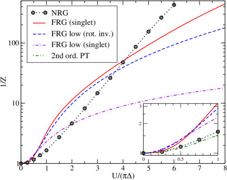
Figure 3: (Color online) Inverse quasiparticle weight $Z^{-1}$ at zero temperature on a logarithmic scale, as a function of $U/(\pi\Delta)$. The inset shows the weak-coupling behavior in the regime $0<U/(\pi\Delta)<1$ on a larger scale. The present FRG method corresponds to the solid curve, the dashed and dot-dashed curves are the FRG results of Ref. [Bartosch09, ], the black circles represent the NRG data and the dot-dot-dashed curve in the inset is the second order perturbation theory.

Finally, in Fig. 3 we show the inverse quasiparticle weight at $T=0$ as a function of the interaction. Unfortunately, in contrast to the NRG results, at strong coupling our FRG method is not able to reproduce the exponential narrowing of the quasiparticle peak predicted by the Bethe Ansatz. Tsvelick83 However, the numerical estimate of $1/Z$ for large values of $U/(\pi\Delta)$ is improved compared to the previous FRG results presented in Ref. [Bartosch09, ]. Fig. 3 shows also clearly the above mentioned overestimation of the interaction in the intermediate coupling regime, characterized by a stronger renormalization of the quasiparticle peak.

VI Conclusions

In the present work we have calculated the spectral function of the symmetric Anderson impurity model at zero and finite temperatures using functional and numerical renormalization group methods. In particular, we took advantage of our high quality NRG data in order to test the validity of the FRG truncation scheme proposed in Ref. [Bartosch09, ], where the on-site interaction is decoupled in the spin-singlet particle-hole channel by means of a bosonic Hubbard-Stratonovich field and an infrared cutoff is explicitly introduced only into the bosonic propagator. Following Ref. [Bartosch09, ], we neglected the FRG flow of vertex functions in order to truncate the infinite hierarchy of FRG flow equations and obtain a closed integro-differential equation for the flowing self-energy $\Sigma_{\Lambda}(i\omega)$. In contrast to Ref. [Bartosch09, ], however, where only the low-energy expansion of the self-energy was taken into account, we solved numerically the integro-differential equation for $\Sigma_{\Lambda}(i\omega)$ keeping the complete frequency structure. This has allowed us to calculate the spectral function at all energy scales, including the high-energy Hubbard bands.

Comparing the FRG results to the NRG data, we found that our truncation scheme gives quantitatively good results for the spectral line-shape in the weak and strong coupling regimes, both at zero and finite temperatures, although it somewhat overestimates the effects of the interaction at intermediate couplings $U/(\pi\Delta)\approx 1$. Most important, in contrast to purely fermionic FRG approaches Hedden04 ; Karrasch08 where no Hubbard-Stratonovich fields are introduced, our method gives an accurate description of both the low-energy and high-energy features of the spectral function, including the correct position and width of the high-energy Hubbard bands in the strong coupling regime.

Unfortunately, our FRG truncation scheme is still not able to correctly reproduce, at zero temperature, the exponential narrowing of the Kondo peak in the strong coupling regime. Most likely, such a non-perturbative effect requires exact symmetry relations, e.g. Ward identities, Kopietz10b to be enforced throughout the integration of the FRG flow.

References

- (1) D. Goldhaber-Gordon, H. Shtrikman, D. Mahalu, D. Abusch-Magder, U. Meirav, and M. A. Kastner, Nature 391, 156 (1998).
- (2) S. M. Cronenwett, T. H. Oosterkamp, and L. P. Kouwenhoven, Science 281, 540 (1998).
- (3) A. Georges, G. Kotliar, W. Krauth, and M. Rozenberg, Rev. Mod. Phys. 68, 13 (1996).
- (4) W. Metzner and D. Vollhardt, Phys. Rev. Lett. 62, 324 (1989).
- (5) A. C. Hewson, The Kondo Problem to Heavy Fermions, (Cambridge University Press, Cambridge, 1993).
- (6) A. M. Tsvelik and P. B. Wiegmann, Adv. Phys. 32, 453 (1983).
- (7) K. G. Wilson, Rev. Mod. Phys. 47, 773 (1975).
- (8) T. A. Costi, A. C. Hewson, and V. Zlatic, J. Phys.: Cond. Mat. 6, 2519 (1994).
- (9) W. Hofstetter, Phys. Rev. Lett. 85, 1508 (2000).
- (10) R. Peters, T. Pruschke, and F. B. Anders, Phys. Rev. B. 74, 245114 (2006).
- (11) A. Weichselbaum and J. von Delft, Phys. Rev. Lett. 99, 076402 (2007).
- (12) R. Bulla, T. Costi, and T. Pruschke, Rev. Mod. Phys. 80, 395 (2008).
- (13) R. Hedden, V. Meden, T. Pruschke, and K. Schönhammer, J. Phys.: Cond. Mat. 16, 5279 (2004).
- (14) C. Karrasch, R. Hedden, R. Peters, T. Pruschke, K. Schönhammer, and V. Meden, J. Phys.: Cond. Mat. 20, 345205 (2008).
- (15) L. Bartosch, H. Freire, J. J. R. Cardenas, and P. Kopietz, J. Phys.: Cond. Mat. 21, 305602 (2009).
- (16) S. G. Jakobs, M. Pletyukhov, and H. Schoeller, arXiv:0911.5502v1 [cond-mat.str-el] (2009).
- (17) J. Berges, N. Tetradis, and C. Wetterich, Phys. Rep. 363, 223 (2002).
- (18) J. M. Pawlowski, Ann. Phys. 322, 2831 (2007).
- (19) P. Kopietz, L. Bartosch, and F. Schütz, Introduction to the Functional Renormalization Group, (Springer, Heidelberg, 2010).
- (20) O. J. Rosten, arXiv:1003.1366v1 [hep-th] (2010).
- (21) L. Bartosch, P. Kopietz and A. Ferraz, Phys. Rev. B 80 , 104514 (2009).
- (22) F. Schütz, L. Bartosch, and P. Kopietz, Phys. Rev. B 72, 035107 (2005).
- (23) S. Floerchinger and C. Wetterich, Phys. Rev. A 77, 053603 (2008).
- (24) P. Strack, R. Gersch, and W. Metzner, Phys. Rev. B 78, 014522 (2008).
- (25) S. Diehl, S. Floerchinger, H. Gies, J. M. Pawlowski, and C. Wetterich, arXiv:0907.2193v1 [cond-mat.quant-gas] (2009).
- (26) D. Litim, Phys. Rev. D 64, 105007 (2001).
- (27) H. J. Vidberg and J. W. Serene, J. Low Temp. Phys. 29, 179 (1977).
- (28) H. R. Krishna-murthy, J. W. Wilkins, and K. G. Wilson, Phys. Rev. B. 21, 1003 (1980); ibid. 21, 1044 (1980).
- (29) M. Yoshida, M. A. Whitaker, and L. N. Oliveira, Phys. Rev. B. 41, 9403 (1990).
- (30) F. B. Anders and A. Schiller, Phys. Rev. Lett. 95, 196801 (2005); Phys. Rev. B. 74, 245113 (2006).
- (31) R. Bulla, A. C. Hewson, and T. Pruschke, J. Phys.: Cond. Mat. 10, 8365 (1998).
- (32) P. Kopietz, L. Bartosch, L. Costa, A. Isidori, and A. Ferraz, arXiv:1003.1867v1 [cond-mat.str-el] (2010).