Spin dynamics in electron-doped pnictide superconductors

Abstract

The doping dependence of spin excitations in Ba(Fe_1-xCo_x)₂As₂ is studied based on a two-orbital model under RPA approximation. The interplay between the spin-density-wave (SDW) and superconductivity (SC) is considered in our calculation. Our results for the spin susceptibility are in good agreement with neutron scattering (NS) experiments in various doping ranges at temperatures (T) above and below the superconducting transition temperature T_c. For the overdoped sample where one of the two hole pockets around $\Gamma$ point disappears according to ARPES, we show that the imaginary part of the spin susceptibility in both SC and normal phases exhibits a gap-like behavior. This feature is consistent with the “pseudogap” as observed by recent NMR and NS experiments.

The recent discovery of the iron arsenide superconductors I1 , whose parent compounds exhibit long-range antiferromagnetic (AF) or spin-density-wave (SDW) order similar to the cuprates I2 , provides another promising group of materials for studying the interplay between magnetism and superconductivity (SC). Especially, the electron-doped pnictide superconductors like Ba(Fe_1-xCo_x)₂As₂ I3 has emerged as one of the most important systems due to the availability of large homogeneous single crystals. The phase diagram I4 ; I5 ; I6-1 for these materials indicates that the parent compound upon cooling through T${}_{N}\sim$ 140K I7 develops a static SDW order. Increasing the doping of Co, the SDW order is suppressed and the SC order emerges as the temperature (T) falls below T_c. The SDW and SC orders coexist in the underdoped samples I4 ; I5 ; I6-1 ; I10 . By further increasing the Co concentration to the optimally doped regime, the SDW order disappears. These experimental results provide compelling evidences for strong competition between the SDW and SC orders.

Recently, several neutron scattering (NS) experiments have been carried out to probe the spin dynamics in these materials I4 ; I6-1 ; I10 ; I12 ; I13 ; I14 ; I15 ; I16 ; I17 ; I18 , and the spin excitation spectrum was fitted by using a $J_{1},J_{2}$ Heisenberg model based on localized spins I12 ; I10 ; I18 . However, while the parent compounds of the cuprates are Mott insulators with large in-plane exchange interactions I19 , the parent iron arsenides are bad metals and remain itinerant at all doping levels. Magnetism in these materials are most likely to originate from itinerant electrons and the AF order is a result of SDW instability due to Fermi-surface nesting I20 . Theoretically, at present, the variation of the spin susceptibility with doping remains less explored. The spin susceptibilities were mostly studied in the optimally doped compounds without SDW I21 or in the parent compound without SC I21-1 . In this work, we adopt Fermi-liquid mean field (MF) theory to study the static SDW and SC, and employ the random-phase approximation (RPA) to investigate the spin dynamics in Ba(Fe_1-xCo_x)₂As₂ from the imaginary part of the dynamic spin susceptibility. It is expected that the present approach is much more justified than the localized model for examining the spin fluctuations in the iron arsenides, as suggested by both experiments I13 ; I16 and theories I21 ; I21-1 . We show that the calculated spin susceptibilities are in qualitative agreement with several NS and NMR experiments in various doping ranges.

We start with a two-orbital model by taking into account two Fe ions per unit cell M1 . The reason we adopt this model is its ability M4 to qualitatively account for the doping evolution of the Fermi surface and the asymmetry in the SC coherent peaks as observed by the angle resolved photo-emission spectroscopy (ARPES) M2 and the scanning tunneling microscopy (STM) M3 experiments on Ba(Fe_1-xCo_x)₂As₂. The Hamiltonian of our system can be expressed as M4 $H=H_{0}+H_{\Delta}+H_{int}$. $H_{0}$ is the tight-binding Hamiltonian and can be written as $H_{0}=\sum_{\mathbf{k}\sigma}\psi_{\mathbf{k}\sigma}^{{\dagger}}M_{\mathbf{k}}\psi_{\mathbf{k}\sigma}$ M1 ; M4 , where $\psi_{\mathbf{k}\sigma}^{{\dagger}}=(c_{A0,\mathbf{k}\sigma}^{{\dagger}},c_{A1,\mathbf{k}\sigma}^{{\dagger}},c_{B0,\mathbf{k}\sigma}^{{\dagger}},c_{B1,\mathbf{k}\sigma}^{{\dagger}})$ is the creation operator with spin $\sigma=-1$ ($\downarrow$) or $1$ ($\uparrow$), in the orbitals $(0,1)=(d_{xz},d_{yz})$ at the sublattice $A$ ($B$), and

$$M_{\mathbf{k}}=\begin{pmatrix}\varepsilon_{A,\mathbf{k}}-\mu&\varepsilon_{xy,\mathbf{k}}&\varepsilon_{T,\mathbf{k}}&0\\ \varepsilon_{xy,\mathbf{k}}&\varepsilon_{A,\mathbf{k}}-\mu&0&\varepsilon_{T,\mathbf{k}}\\ \varepsilon_{T,\mathbf{k}}&0&\varepsilon_{B,\mathbf{k}}-\mu&\varepsilon_{xy,\mathbf{k}}\\ 0&\varepsilon_{T,\mathbf{k}}&\varepsilon_{xy,\mathbf{k}}&\varepsilon_{B,\mathbf{k}}-\mu\end{pmatrix},$$ (1)

where $\varepsilon_{A,\mathbf{k}}=-2(t_{2}\cos k_{x}+t_{3}\cos k_{y})$, $\varepsilon_{B,\mathbf{k}}=-2(t_{2}\cos k_{y}+t_{3}\cos k_{x})$, $\varepsilon_{xy,\mathbf{k}}=-2t_{4}(\cos k_{x}+\cos k_{x})$, and $\varepsilon_{T,\mathbf{k}}=-4t_{1}\cos\frac{k_{x}}{2}\cos\frac{k_{y}}{2}$. $t_{1-4}$ are the hopping parameters and $\mu$ is the chemical potential. Throughout the paper, the momentum $\mathbf{k}$ is defined in the tetragonal notation.

The pairing term is $H_{\Delta}=\sum_{\mathbf{k}s\alpha}(\Delta_{\mathbf{k}}c_{s\alpha,\mathbf{k}\uparrow}^{{\dagger}}c_{s\alpha,-\mathbf{k}\downarrow}^{{\dagger}}+h.c.)$. Here, we assume there exits only next-nearest-neighbor intraorbital pairing with extended $s-$wave pairing symmetry, and the SC order parameter is $\Delta_{\mathbf{k}}=\frac{\Delta_{0}}{2}(\cos k_{x}+\cos k_{y})$ similar to that obtained by spin fluctuations I20 , where

$$\Delta_{0}=\frac{2V_{nnn}}{N}\sum_{\mathbf{k}}(\cos k_{x}+\cos k_{y})\langle c_{s\alpha,-\mathbf{k}\downarrow}c_{s\alpha,\mathbf{k}\uparrow}\rangle,$$ (2)

with $V_{nnn}$ being the attractive pairing interaction.

$H_{int}$ is the on-site interaction term which includes the Coulombic interaction and Hund coupling $J_{H}$, following Refs. M4 ; M5 ; I21 , it can be expressed as

$$H_{int}= U \sum_{ijs\alpha}n_{s\alpha,ij\uparrow}n_{s\alpha,ij\downarrow}+(U^{{}^{\prime}}-\frac{J_{H}}{2})\sum_{ijs}n_{s0,ij}n_{s1,ij}$$ (3)

$$+ J_{H}\sum_{ijs}(c_{s0,ij\uparrow}^{{\dagger}}c_{s0,ij\downarrow}^{{\dagger}}c_{s1,ij\downarrow}c_{s1,ij\uparrow}+h.c.)$$

$$- 2J_{H}\sum_{ijs}\mathbf{S}_{s0,ij}\cdot\mathbf{S}_{s1,ij},$$

where $\{i,j\}$ denotes the unit cell, $s=0$ ($A$) or $1$ ($B$) is the sublattice index, and $\alpha=0$ ($d_{xz}$) or $1$ ($d_{yz}$) represents the orbital. $n_{s\alpha,ij\sigma}$ and $\mathbf{S}_{s\alpha,ij}$ are the density and spin operators in the orbital $\alpha$ at the sublattice $s$ of the unit cell $\{i,j\}$, respectively. According to symmetry, we have $U^{{}^{\prime}}=U-2J_{H}$ M5 . In the MF approach, we linearize $H_{int}$ in momentum space as M4 ; M6

$$H_{int}^{MF} = \frac{n}{4}(3U-5J_{H})\sum_{\mathbf{k}s\alpha\sigma}n_{s\alpha,\mathbf{k}\sigma}$$ (4)

$$- \frac{m}{2}(U+J_{H})\sum_{\mathbf{k}s\alpha\sigma}\sigma c_{s\alpha,\mathbf{k}+\mathbf{Q}\sigma}^{{\dagger}}c_{s\alpha,\mathbf{k}\sigma},$$

where $n=2+x$ is the number of electrons per lattice site and $\mathbf{Q}=(\pi,\pi)$. The SDW order parameter is $m=\frac{1}{N}\sum_{\mathbf{k}\sigma}\sigma\langle c_{s\alpha,\mathbf{k}+\mathbf{Q}\sigma}^{{\dagger}}c_{s\alpha,\mathbf{k}\sigma}\rangle$, with $N$ being the number of unit cells.

The effective MF Hamiltonian is then given by

$$H^{MF} = \sum_{\mathbf{k}}\hskip 0.56905pt^{\prime}\varphi_{\mathbf{k}}^{{\dagger}}W_{\mathbf{k}}\varphi_{\mathbf{k}},$$

$$W_{\mathbf{k}} = \begin{pmatrix}M_{\mathbf{k}}^{{}^{\prime}}&R&\Delta_{\mathbf{k}}I&0\\ R&M_{\mathbf{k}+\mathbf{Q}}^{{}^{\prime}}&0&-\Delta_{\mathbf{k}}I\\ \Delta_{\mathbf{k}}I&0&-M_{\mathbf{k}}^{{}^{\prime}}&R\\ 0&-\Delta_{\mathbf{k}}I&R&-M_{\mathbf{k}+\mathbf{Q}}^{{}^{\prime}}\end{pmatrix},$$ (5)

where $\varphi_{\mathbf{k}}^{{\dagger}}=(\psi_{\mathbf{k}\uparrow}^{{\dagger}},\psi_{\mathbf{k}+\mathbf{Q}\uparrow}^{{\dagger}},\psi_{-\mathbf{k}\downarrow},\psi_{-(\mathbf{k}+\mathbf{Q})\downarrow})$, $M_{\mathbf{k}}^{{}^{\prime}}=M_{\mathbf{k}}+\frac{n}{4}(3U-5J_{H})I$, and $R=-\frac{m}{2}(U+J_{H})I$. $I$ is a $4\times 4$ unit matrix and $\sum_{\mathbf{k}}^{{}^{\prime}}$ means the summation extends over the magnetic Brillouin zone (MBZ): $-\pi<k_{x}\pm k_{y}\leqslant\pi$. The MF Green’s function matrix can be written as $g(\mathbf{k},\tau)=-\langle T_{\tau}\varphi_{\mathbf{k}}(\tau)\varphi_{\mathbf{k}}^{{\dagger}}(0)\rangle$ and $g(\mathbf{k},ip_{n})=A_{\mathbf{k}}W_{\mathbf{k}}^{{}^{\prime}}A_{\mathbf{k}}^{{\dagger}}$, where $W_{\mathbf{k}ij}^{{}^{\prime}}=\delta_{ij}(ip_{n}-\lambda_{\mathbf{k}i})^{-1}$ and $A_{\mathbf{k}}$ is a unitary matrix that satisfies $(A_{\mathbf{k}}^{{\dagger}}W_{\mathbf{k}}A_{\mathbf{k}})_{ij}=\delta_{ij}\lambda_{\mathbf{k}i}$.

First, we solve the MF equations self-consistently to obtain $m$, $\Delta_{0}$ and $\mu$ at different doping levels $x$ and temperatures $T$. The magnitudes of the parameters are chosen as $t_{1-4}=1,0.4,-2,0.04$ M1 , $U=3.4$, $J_{H}=1.3$, $V_{nnn}=-1.2$ M4 , and the number of unit cells is $257\times 257$. Throughout the paper, the energies are measured in units of $|t_{1}|$. The calculated phase diagram as shown in the inset of Fig. 1(a) reproduces the result based on Bogoliubov-de Gennes (BdG) equations M4 and is also consistent with the experiments on Ba(Fe_1-xCo_x)₂As₂ I4 ; I5 ; I6-1 . Here the SDW and SC are competing with each other. If there is no SDW, SC would show up even in the parent compound. The presence of SC also suppresses SDW. For example, in the underdoped ($x=0.06$) compound with $T_{N}\approx 0.16$ and $T_{c}\approx 0.05$, the calculated magnitude of $m^{2}$ (proportional to the magnetic Bragg peak intensity) at $T=0$ is reduced by $\sim 4\%$ relative to that of the maximum intensity at $T_{c}$ [see Fig. 1(a)], and this result is consistent with the neutron diffraction experiments I4 ; I10 .

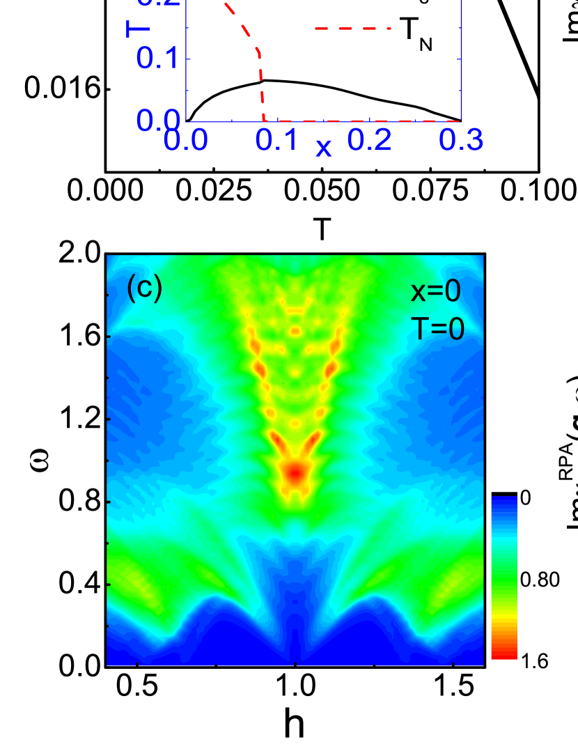
Figure 1: (Color online) (a) $m^{2}$ as a function of $T$ close to $T_{c}$ at $x=0.06$. Inset shows the calculated phase diagram. (b) $Im\chi^{RPA}(\mathbf{q},\omega)$ at $\mathbf{q}=(\pi,\pi)$ as a function of $\omega$ by changing $i\omega_{n}$ to $\omega+i\eta$, at $x=0$ and different temperatures $T$. (c) $Im\chi^{RPA}(\mathbf{q},\omega)$ as a function of energy transfer $\omega$ and momentum $\mathbf{q}$, at $x=0$ and $T=0$. The momentum is scanned along $(q_{x}/\pi,q_{y}/\pi)=(h,h)$. (d) Constant-energy scans along the $(q_{x}/\pi,q_{y}/\pi)=(h,h)$ direction at $x=0$ and $T=0$. Successive cuts are displaced vertically for clarity. The energy transfer is $\omega=0.09$ (black solid), $0.4$ (red dash), $0.93$ (green dot), $1.2$ (blue dash dot), and $2$ (cyan short dash). The damping rate $\eta=0.04$.

Then, we investigate the spin dynamics in Ba(Fe_1-xCo_x)₂As₂ for $x=0$, $0.06$, $0.1$, and $0.2$, corresponding to the undoped, underdoped, optimally doped and overdoped compounds, respectively. The MF spin susceptibility is $\chi^{r\alpha,s\beta(0)}_{t\gamma,u\delta}(\mathbf{q},\mathbf{q}^{{}^{\prime}},i\omega_{n})=\frac{\delta_{\mathbf{q}^{{}^{\prime}},\mathbf{q}}}{2}\sum_{(i,j)=(p,o)}^{(o+8,p+8)}[P_{im,nj}(q)+P_{i+4m,nj+4}(q)]$, here, $r,s,t,u$ label the sublattice indices, $\alpha,\beta,\gamma,\delta$ represent the orbitals, $m=2r+\alpha+1,n=2s+\beta+1,o=2t+\gamma+1,p=2u+\delta+1$, and $P_{im,nj}(q)=-\frac{1}{\beta N}\sum_{\mathbf{k},p_{n}}g_{im}(k)g_{nj}(k+q)$. Here we used $k=(\mathbf{k},ip_{n})$ and $q=(\mathbf{q},i\omega_{n})$.

We then use RPA to take into account the residual fluctuation of $H_{int}$ beyond MF. The RPA spin susceptibility is determined by the matrix equation $\chi^{RPA}(q)=\sum_{rt\alpha\gamma}\{\chi^{0}(q)[I-\Gamma\chi^{0}(q)]^{-1}\}^{r\alpha,r\alpha}_{t\gamma,t\gamma}$, where $I$ is a $16\times 16$ unit matrix and the nonzero elements of the interaction vertex are: for $\alpha=\beta=\gamma=\delta$, $\Gamma^{r\alpha,r\beta}_{r\gamma,r\delta}=2U$; for $\alpha=\beta\neq\gamma=\delta$ or $\alpha=\gamma\neq\beta=\delta$, $\Gamma^{r\alpha,r\beta}_{r\gamma,r\delta}=2J_{H}$.

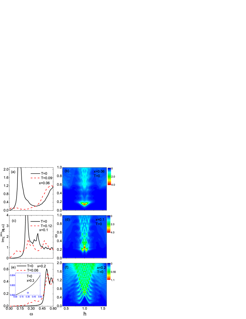
Figure 2: (Color online) (a) $Im\chi^{RPA}(\mathbf{q},\omega)$ at $\mathbf{q}=(\pi,\pi)$ as a function of $\omega$, at $x=0.06$ and different temperatures $T$. (b) $Im\chi^{RPA}(\mathbf{q},\omega)$ as a function of energy transfer $\omega$ and momentum $\mathbf{q}$, at $x=0.06$ and $T=0$. The momentum is scanned along $(q_{x}/\pi,q_{y}/\pi)=(h,h)$. (c) and (d) ((e) and (f)) are similar to (a) and (b), respectively, but at $x=0.1$ ($x=0.2$). Inset in (e) shows the $x=0.3$ case.

In the parent ($x=0$) compound, the RPA spin susceptibility [see Fig. 1(b)] in the paramagnetic state at $T=0.27$ ($T_{N}\approx 0.25$) shows a linear energy dependence for $\omega<0.1$, suggesting gapless excitations I13 ; I17 . On the other hand, in the SDW state at $T=0$, the spin excitation intensity is close to zero below $\omega\approx 0.13$, similar to a spin gap I13 ; I12 . However, the gap is not sharp since a sharp gap would produce a stepwise increase in intensity at the gap energy which is unlike the more gradual increase seen here. Figures 1(c) and 1(d) show $Im\chi^{RPA}(\mathbf{q},\omega)$ as a function of energy transfer $\omega$ and momentum $\mathbf{q}$ along $(q_{x}/\pi,q_{y}/\pi)=(h,h)$ direction at $T=0$. As we can see, there is almost no detectable intensity below $\omega\approx 0.13$, again illustrating the opening of the spin gap. The excitations are peaked at $\mathbf{Q}=(\pi,\pi)$ and $\omega\approx 0.93$, at higher energies, the response is seen to split and broaden due to the dispersion of the spin waves. By tracking the peak positions in Fig. 1(c), the spin-wave dispersion relation can be fitted as $\omega_{q}=\sqrt{\Delta^{2}+v^{2}q^{2}}$ I11 ; I13 ; I18 , where $\Delta\approx 0.93$ is an energy gap, $v\approx 9.02$ is the spin-wave velocity, and $q$ is the reduced wave vector away from $(1,1)$ along the $(h,h)$ direction, consistent with the experimental observations I12 ; I13 . The origin of the spin gap can be understood in terms of the Fermi surface at $x=0$ as shown in Fig. 2(a) in Ref. M4 . In the paramagnetic state, large parts of the two hole pockets around $\Gamma=(0,0)$ and two electron pockets around $M=(\pi,\pi)$ are nested by momentum $(\pi,\pi)$, thus giving rise to the gapless excitations at $T=0.27$. But at $T=0$, the SDW order will gap most parts of the original Fermi surface, leaving only tiny ungapped Fermi surface pockets connected by $(\pi,\pi)$ along the $\Gamma-M$ line, so in this case, for small energies, the imaginary part of the MF spin susceptibility is close to zero, while its real part does not fulfill the resonance condition, leading to a spin gap opening in the RPA spin susceptibility.

The RPA spin susceptibility [Fig. 2(a)] at $x=0.06$ suggests that the excitations above $T_{c}$ are gapless, although the intensity is very small at low energy. This may be the reason why above $T_{c}$, Ref. I4 claims the excitations are gapless while Ref. I10 concludes they are gapped. Below $T_{c}$, the intensities below $\omega\approx 0.06$ and above $\omega\approx 0.36$ are suppressed and the weight is transferred to form a resonance at $\omega_{res}\approx 0.14$. Since $m(T=0.09)\approx 0.129$ and $m(T=0)\approx 0.131$, our results seem to agree with Ref. I4 , which claims the resonance is produced by suppressing low energy spectral weight, rather than Ref. I10 , where the spectral weight is considered to be transferred from the ordered magnetic moments. In addition, figure 2(b) shows that below $\omega_{res}$, commensurate spin excitation prevails, in agreement with experimental observation I10 , and it becomes incommensurate when the energy is above $\omega_{res}$, notably between $\omega\approx 0.15$ and $\omega\approx 0.18$, which we predict to be measurable by NS experiment. The spin excitations can extend beyond $\omega=1$, with smeared out and broadened features for $\omega\gtrsim 0.2$.

At $x=0.1$, the SDW order is completely suppressed, and SC emerges for $T<T_{c}\approx 0.06$. The excitation spectrum [Fig. 2(c)] shows that in the superconducting state at $T=0$, a gap below $\omega\approx 0.08$ develops and there is a resonance above the gap energy peaking at $\omega_{res}\approx 0.24$, in agreement with the NS experiments on the optimally doped Ba(Fe_1-xCo_x)₂As₂ I15 ; I16 ; I14 ; I17 . Furthermore, figure 2(d) shows that the spin excitation is incommensurate at low energy ($0.18\lesssim\omega\lesssim\omega_{res}$) which still need to be verified by experiments, then it switches to a commensurate behavior between $\omega\approx\omega_{res}$ and $\omega\approx 0.3$, and becomes broad at higher energy, consistent with Refs. I18 ; I15 ; I16 . In the normal state at $T=0.12$, the spectrum is replaced by broad gapless excitations with a linear energy dependence for $\omega<0.1$ I16 ; I17 . We notice a marked similarity between the spin excitations in the normal state of the optimally doped compound and those in the paramagnetic state of the parent compound as observed in Ref. I17 , suggesting a common origin of spin fluctuations in both of them.

In contrast, the spin excitations in the overdoped ($x=0.2$) compound [Fig. 2(e)] show gap-like behavior in both the normal and superconducting states. The origin of the gap may be due to one of the two hole pockets around $\Gamma$ vanishes and the other one shrinks dramatically in the overdoped region according to ARPES experiments M2 and theories M1 ; M4 . Under such a case, due to the lack of interband scattering between the hole and electron pockets, the imaginary part of the spin susceptibility is strongly suppressed and gives rise to the pseudogap behavior R1 which has been observed in NMR R2 and NS I17 experiments in the electron overdoped Ba(Fe_1-xCo_x)₂As₂. But in Ref. R1 , the pseudogap is associated with the vanishing of one of three hole pockets around $\Gamma$, where experimentally there is only one hole pocket at this doping level as observed by ARPES M2 . The spin excitations in the superconducting state at $T=0$ [Fig. 2(f)] are broader and weaker than those in the underdoped and optimally doped compounds, suggesting the importance of the hole pocket in enhancing the spin fluctuations.

At $x=0.3$, both the two hole pockets around $\Gamma$ disappear M1 ; M4 , our calculations show that SC is completely suppressed and the spin fluctuations are extremely small [The inset of Fig. 2(e)]. This further indicates the correlation between the electronic band structure and magnetism, and supports the scenario that the spin fluctuations in the underdoped regime, which serve as a precursor to SC, originate from quasiparticle scattering across the electron and hole pockets.

In summary, we have systematically investigated the doping dependence of spin excitations in Ba(Fe_1-xCo_x)₂As₂, ranging from the parent to overdoped regime. In the parent compound, the spin excitations are gapless in the paramagnetic state and become strongly suppressed at low energy in the SDW state due to the opening of gaps on most parts of the original Fermi surface. For underdoped and optimally doped samples, the spin gaps and resonances at $(\pi,\pi)$ only occur in the SC state. On the other hand, the spin excitations in the overdoped compound show gap-like behavior in both the normal and SC states due to the vanishing of one hole pocket around $\Gamma$, leading to a “pseudogap” behavior at this doping level. All the obtained results are in qualitative agreement with experiments. The changes in the spin dynamics at different doping levels may reflect changes in the electronic band structure and suggest a strong correlation between SC and magnetism.

Acknowledgments We thank D. G. Zhang, C. H. Li, J. P. Hu and J. X. Zhu for helpful discussions. This work was supported by the Texas Center for Superconductivity and the Robert A. Welch Foundation under grant numbers E-1070 (Yi Gao and W.P. Su) and E-1146 (Tao Zhou and C. S. Ting).

References

- (1) Y. Kamihara, T. Watanabe, M. Hirano, and H. Hosono, J. Am. Chem. Soc. 130, 3296 (2008).
- (2) P. A. Lee, N. Nagaosa, and X. -G. Wen, Rev. Mod. Phys. 78, 17 (2006), and references therein.
- (3) A. S. Sefat et al., Phys. Rev. Lett. 101, 117004 (2008).
- (4) D. K. Pratt et al., Phys. Rev. Lett. 103, 087001 (2009).
- (5) J. H. Chu et al., Phys. Rev. B 79, 014506 (2009); F. Ning et al., J. Phys. Soc. Jpn. 78, 013711 (2009).
- (6) C. Lester et al., Phys. Rev. B 79, 144523 (2009).
- (7) M. Rotter, M. Tegel, and D. Johrendt, Phys. Rev. Lett. 101, 107006 (2008); G. Wu et al., Europhys. Lett. 84, 27010 (2008); M. Rotter, M. Tegel, and D. Johrendt, Phys. Rev. B 78, 020503(R) (2008).
- (8) A. D. Christianson et al., Phys. Rev. Lett. 103, 087002 (2009).
- (9) R. A. Ewings et al., Phys. Rev. B 78, 220501(R) (2008).
- (10) K. Matan et al., Phys. Rev. B 79, 054526 (2009).
- (11) D. Parshall et al., Phys. Rev. B 80, 012502 (2009).
- (12) M. D. Lumsden et al., Phys. Rev. Lett. 102, 107005 (2009).
- (13) D. S. Inosov et al., Nature Physics 6, 178 (2010).
- (14) K. Matan et al., arXiv:0912.4945 (2009).
- (15) C. Lester et al., Phys. Rev. B 81, 064505 (2010).
- (16) M. A. Kastner et al., Rev. Mod. Phys. 70, 897 (1998).
- (17) I. I. Mazin et al., Phys. Rev. Lett. 101, 057003 (2008).
- (18) M. M. Korshunov and I. Eremin, Phys. Rev. B 78, 104509 (2008); T. A. Maier and D. J. Scalapino, Phys. Rev. B 78, 020514(R) (2008).
- (19) J. Knolle, I. Eremin, A.V. Chubukov, and R. Moessner, arXiv:1002.1668 (2010).
- (20) Degang Zhang, Phys. Rev. Lett. 103, 186402 (2009).
- (21) T. Zhou, Degang Zhang, and C. S. Ting, Phys. Rev. B 81, 052506 (2010).
- (22) K. Terashima et al., Proc. Natl. Acad. Sci. U.S.A. 106, 7330 (2009); Y. Sekiba et al., New J. Phys. 11, 025020 (2009).
- (23) S. H. Pan et al., private communication.
- (24) A. M. Oles et al., Phys. Rev. B 72, 214431 (2005).
- (25) Z. Y. Weng, T. K. Lee, and C. S. Ting, Phys. Rev. B 38, 6561 (1988); J. R. Schridffer, X. G. Wen, and S. C. Zhang, Phys. Rev. B 39, 11663 (1989).
- (26) R. J. McQueeney et al., Phys. Rev. Lett. 101, 227205 (2008); S. O. Diallo et al., Phys. Rev. Lett. 102, 187206 (2009).
- (27) H. Ikeda, R. Arita, and J. Kuneš, arXiv:1002.4471 (2010), Phys. Rev. B 81, 054502 (2010).
- (28) F. L. Ning et al., Phys. Rev. Lett. 104, 037001 (2010).