Morphological instability, evolution, and scaling in strained epitaxial films: An amplitude equation analysis of the phase field crystal model

Abstract

Morphological properties of strained epitaxial films are examined through a mesoscopic approach developed to incorporate both the film crystalline structure and standard continuum theory. Film surface profiles and properties, such as surface energy, liquid-solid miscibility gap and interface thickness, are determined as a function of misfit strains and film elastic modulus. We analyze the stress-driven instability of film surface morphology that leads to the formation of strained islands. We find a universal scaling relationship between the island size and misfit strain which shows a crossover from the well-known continuum elasticity result at the weak strain to a behavior governed by a “perfect” lattice relaxation condition. The strain at which the crossover occurs is shown to be a function of liquid-solid interfacial thickness, and an asymmetry between tensile and compressive strains is observed. The film instability is found to be accompanied by mode coupling of the complex amplitudes of the surface morphological profile, a factor associated with the crystalline nature of the strained film but absent in conventional continuum theory.

I Introduction

The most recent area of focus in thin film epitaxy has been on exploiting the growth and control of strained solid films to develop specific nanostructure features that can be used in optoelectronic device applications. These structures include junctions, quantum wells, and multilayers/superlattices for which planar interfaces are highly desired. On the other hand, epitaxially grown films are usually strained due to the lattice mismatch with the substrate, leading to a variety of stress-induced effects and structures either on the film surface or across the interfaces, such as islands (quantum dots) or nanowires. Stangl et al. (2004); Shchukin and Bimberg (1999); Teichert (2002); Berbezier and Ronda (2009) A wide range of device applications results from such heterostructures, including LEDs, diode lasers, detectors, FETs, etc., Humphreys (2008); Stangl et al. (2004) with the major technical concerns being the requirement of long-range ordering, size regularity, placement and defect control.

Much progress has been made in understanding film growth above the surface roughening temperature, particularly the formation and evolution of coherent nanostructures. The evolution sequence often involves many physical processes, including an initial morphological instability of the Asaro-Tiller-Grinfeld (ATG) type Asaro and Tiller (1972); Grinfeld (1986); Srolovitz (1989); Spencer et al. (1991, 1993) that results in surface ripples and undulations, Sutter and Lagally (2000); Tromp et al. (2000) the formation of islands and the evolution from pre-pyramid to faceted shape (e.g., $\{105\}$-faceted pyramids for SiGe Tersoff et al. (2002)), subsequent islands coarsening, Ross et al. (1998); Floro et al. (2000); Rastelli et al. (2005) further shape transitions from pyramids to domes Ross et al. (1998) or to unfaceted prepyramids Rastelli et al. (2005) and the nucleation of misfit dislocations for very large islands. Jesson et al. (1995); Albrecht et al. (1995)

To understand these complex processes of nanostructure self-assembly, most of current theoretical efforts are based on either continuum diffusion and elasticity theories or atomistic simulation methods that focus on a certain single scale of description. In standard continuum theory, the film morphology is described by a coarse-grained, continuum surface profile Srolovitz (1989); Spencer et al. (1991) or phase fields, Müller and Grant (1999); Kassner et al. (2001); Wise et al. (2005) with evolution governed by the relaxation of continuum elastic and surface free energies. Quantitative results have been obtained to reveal fundamental mechanisms of film nanostructure formation observed in a variety of experimental systems. Recent work has focused on morphological instabilities of strained films Srolovitz (1989); Spencer et al. (1991, 1993) or superlattices, Shilkrot et al. (2000); Huang and Desai (2003); Huang et al. (2003) the coupling to alloy film composition inhomogeneity, Guyer and Voorhees (1995); Léonard and Desai (1998); Spencer et al. (2001); Huang and Desai (2002a, b) island evolution, Spencer and Blanariu (2005); Tu and Tersoff (2007) ordering and coarsening Müller and Grant (1999); Kassner et al. (2001); Wise et al. (2005); Liu et al. (2001); Levine et al. (2007); Huang et al. (2007) as well as island growth on nanomembranes/nanoribbons. Huang et al. (2009); Kim-Lee et al. (2009) Such continuum approaches give a long-wavelength description of the system, which has a large computational advantage over microscopic approaches but naturally neglects many microscopic crystalline details that can have a significant impact on film structural evolution and defect dynamics. This can be remedied via atomistic simulations such as kinetic Monte Carlo (MC) methods. Recent progress includes identifying detailed properties of strained islands such as morphology, density and size distribution Nandipati and Amar (2006); Zhu et al. (2007) and the evolution of complex surface structures including dots, pits and grooves as a function of growth conditions in both two Lam et al. (2002) and three Lung et al. (2005) dimensions. However to simulate strained film growth, novel approaches (e.g., Green’s function method Lam et al. (2002); Zhu et al. (2007) or local approximation technique Schulze and Smereka (2009)) are required to incorporate strain energy via long-range elastic interactions, which usually limit atomistic studies to small length and time scales.

Recently an approach coined Phase Field Crystal (PFC) modeling has been developed to incorporate atomic-level crystalline structures into standard continuum theory for pure and binary systems. Elder et al. (2002); Elder and Grant (2004); Elder et al. (2004, 2007) This model can be related to other continuum field theories such as classical density functional theory Ramakrishnan and Yussouff (1979); Singh (1991); van Teeffelen et al. (2009); Kahl and Lowen (2009) and the atomic density function theory. Jin and Khachaturyan (2006) The PFC model describes the diffusive, large-time-scale dynamics of the atomic number density field $\rho$, which is spatially periodic on atomic length scales. By including atomic scale variations, the physics associated with elasticity, plasticity, multiple crystal orientations and anisotropic properties (of, e.g., surface energy and elastic constants) is naturally incorporated. This approach has been applied to a wide variety of phenomena including glass formation, Berry et al. (2008) climb and glide dynamics of dislocations, Berry et al. (2006) epitaxial growth, Elder et al. (2002); Elder and Grant (2004); Elder et al. (2007); Huang and Elder (2008); Wu and Voorhees (2009); Yu et al. (2009) pre-melting at grain boundaries, Berry et al. (2008b); Mellenthin et al. (2008) commensurate/incommensurate transitions, Achim et al. (2006); Ramos et al. (2008) sliding friction phenomena Achim et al. (2009) and the yield strength of polycrystals. Elder et al. (2002); Elder and Grant (2004); Hirouchi et al. (2009); Stefanovic et al. (2009) For strained film epitaxy, the basic sequence of film evolution observed in experiments, i.e., morphological instability $\rightarrow$ nanostructure/island formation $\rightarrow$ dislocation nucleation and climb, has been successfully reproduced in PFC simulations. Elder and Grant (2004); Elder et al. (2007); Huang and Elder (2008); Wu and Voorhees (2009) Unfortunately computational simulations of the original PFC model are limited by the need to resolve atomic length scales. This limitation can be overcome by deriving the corresponding amplitude equation formalism as developed by Goldenfeld et al. Goldenfeld et al. (2005); Athreya et al. (2006) to effectively describe the system via the “slow”-scale amplitude and phase of the atomic density $\rho$, while at the same time retaining the key characters (e.g., elasticity, plasticity and multiple crystal orientations) of the modeling. Very recently such a mesoscopic approach has been extended by Yeon et al. Yeon et al. (2010) to incorporate a slowly-varying average density field which is essential to account for the liquid-solid coexistence and a miscibility gap, and also by Elder et al. Elder et al. (2010) to describe the binary alloy systems for both two-dimensional (2D) hexagonal and three-dimensional (3D) bcc and fcc structures. Application of this extended expansion to strained film growth and island formation has yielded promising results, particularly the determination of a universal size scaling of surface nanostructures (strained islands). Huang and Elder (2008) However, in these PFC studies some key factors for understanding the basic mechanisms of strained film evolution are still missing and yet to be addressed, including film surface properties (such as strain-dependent surface tension and width) and the effect of the sign of film/substrate misfit strain, as will be clarified in this work.

In this paper we provide a complete formulation for such multiple-scale analysis of single-component, strained film epitaxy. Compared to our previous work Huang and Elder (2008) which is also based on the amplitude equation formalism established for two-dimensional high temperature growth, here we provide a new and more systematic study of various strained film properties including surface energy, film surface (or liquid-film interface) thickness, and liquid-film miscibility gap that are identified for different misfit strains (both tensile and compressive). Furthermore, morphological instabilities of the strained films and the corresponding behavior of island formation are systematically investigated, showing the important effects of misfit strains (both magnitude and sign) and film surface properties that are absent in previous work. A main feature of our multi-scale (mesoscopic/microscopic) approach is that it can maintain the efficiency advantage of the continuum theory through coarse-grained amplitudes, without losing significant effects due to the discrete nature of the crystalline film structure.

II Amplitude Equation Formalism for Strained Film Epitaxy

In the PFC model, Elder et al. (2002); Elder and Grant (2004); Elder et al. (2007) the free energy functional $F$ can be derived from the classical density functional theory of freezing Elder et al. (2007) and be expressed in terms of a dimensionless atomic number density $n=(\rho-\bar{\rho})/\bar{\rho}$, i.e.,

$$F/\bar{\rho}k_{B}T=\int d{\bm{r}}\left\{\frac{n}{2}\left[B^{\ell}+B^{x}\left(2R^{2}\nabla^{2}+R^{4}\nabla^{4}\right)\right]n-\frac{\tau}{3}n^{3}+\frac{v}{4}n^{4}\right\},$$ (1)

where $\bar{\rho}$ is the average density, $T$ is the temperature, $R$ represents the lattice spacing, $B^{\ell}$ is related to the isothermal compressibility of the liquid phase, $B^{x}$ is proportional to the bulk modulus of the crystalline state, and $\tau$ and $v$ are phenomenological parameters (chosen as $\tau=1/2$, $v=1/3$ in the following calculations for simplicity). The liquid-solid transition is controlled by a parameter $\epsilon=(B^{x}-B^{\ell})/B^{x}$ which is related to temperature difference from the melting point. The solid phase exists at $\epsilon>0$, with hexagonal/triangular crystalline symmetry in 2D and bcc in 3D. Based on the assumption of conserved system dynamics, i.e., $\partial n/\partial t=\Gamma\nabla^{2}\delta F/\delta n$ with $\Gamma$ the mobility, the PFC dynamic equation is given by

$$\partial n/\partial t=\Gamma\nabla^{2}\left[B^{\ell}n+B^{x}(R^{4}\nabla^{4}+2R^{2}\nabla^{2})n-\tau n^{2}+vn^{3}\right].$$ (2)

Defining a length scale $l_{0}=R$, a time scale $\tau_{0}=R^{2}/\Gamma B^{x}$, and $n\rightarrow\sqrt{v/B^{x}}~{}n$, we obtain the rescaled equation

$$\partial n/\partial t=\nabla^{2}\left[-\epsilon\,n+(\nabla^{2}+q_{0}^{2})^{2}n-gn^{2}+n^{3}\right],$$ (3)

where $g=\tau/\sqrt{vB^{x}}$, $q_{0}=1$ and the symbol $q_{0}$ is retained for the clarity of presentation.

For the epitaxial system of interest, we consider a system configuration composed of a semi-infinite strained crystalline film and a coexisting homogeneous liquid state, which are separated by a time-evolving interface (i.e., film surface). To access the “slow” time and length scales of the film surface profile we introduce a standard multiple scale expansion of the PFC equation (3) and derive the associated amplitude equations, with detailed procedures given in Refs. Goldenfeld et al., 2005; Athreya et al., 2006; Yeon et al., 2010. For a 2D system with the film surface normal to the $y$ direction, the atomic density field $n$ is expanded in both liquid and solid regions as the superposition of a spatially/temporally-varying average local density $n_{0}$ (for the zero wavenumber mode) and three hexagonal base modes, i.e.,

$$n=n_{0}(X,Y,T)+\sum\limits_{j=1}^{3}A_{j}(X,Y,T)e^{i{\bm{q}}_{j}^{0}\cdot{\bm{r}}}+{\rm c.c.},$$ (4)

where both $n_{0}$ and complex amplitudes $A_{j}$ are slowly varying variables (with $A_{j}=0$ in the liquid region), and ${\bm{q}}_{j}^{0}$ represent the three hexagonal basic wave vectors

$${\bm{q}_{1}^{0}}=q_{0}\left(-\frac{\sqrt{3}}{2}\hat{x}-\frac{1}{2}\hat{y}\right),\quad{\bm{q}_{2}^{0}}=q_{0}\hat{y},\quad{\bm{q}_{3}^{0}}=q_{0}\left(\frac{\sqrt{3}}{2}\hat{x}-\frac{1}{2}\hat{y}\right).$$ (5)

This expansion (4) implies the separation of “slow” scales $X=\epsilon^{1/2}x$, $Y=\epsilon^{1/2}y$, $T=\epsilon t$ for $n_{0}$ and $A_{j}$ (and hence the film surface profile) from the underlying crystalline structure, at the limit of small $\epsilon$ or high temperature growth. The corresponding amplitude equations are given by (in the form of Model C Hohenberg and Halperin (1977))

$$\partial A_{j}/\partial t=-q_{0}^{2}\delta{\cal F}/\delta A_{j}^{*},$$ (6)

$$\partial n_{0}/\partial t=\nabla^{2}\delta{\cal F}/\delta n_{0},$$ (7)

where the effective potential ${\cal F}$ (a Lyapunov functional) is written as

$${\cal F}= \int d{\bm{r}}\left\{(-\epsilon+3n_{0}^{2}-2gn_{0})\sum_{j=1}^{3}|A_{j}|^{2}+\sum_{j=1}^{3}\left|\left(\nabla^{2}+2i{\bm{q}}_{j}^{0}\cdot{\bm{\nabla}}\right)A_{j}\right|^{2}+\frac{3}{2}\sum_{j=1}^{3}|A_{j}|^{4}\right.$$ (8)

$$+(6n_{0}-2g)(A_{1}A_{2}A_{3}+A_{1}^{*}A_{2}^{*}A_{3}^{*})+6\left(|A_{1}|^{2}|A_{2}|^{2}+|A_{1}|^{2}|A_{3}|^{2}+|A_{2}|^{2}|A_{3}|^{2}\right)$$

$$\left.-\frac{1}{2}\epsilon n_{0}^{2}+\frac{1}{2}\left[\left(\nabla^{2}+q_{0}^{2}\right)n_{0}\right]^{2}-\frac{1}{3}gn_{0}^{3}+\frac{1}{4}n_{0}^{4}\right\}.$$

Note that the operator $(\nabla^{2}+2i{\bm{q}}_{j}^{0}\cdot{\bm{\nabla}})$ preserves the rotational covariance of these amplitude equations. Gunaratne et al. (1994) This effective free energy describes a first order phase transition from a liquid ($A_{j}=0$) to a solid state ($A_{j}\neq 0$) and incorporates elasticity though the operator $(\nabla^{2}+2i{\bm{q}}_{j}^{0}\cdot{\bm{\nabla}})$, as discussed in Ref. Elder et al., 2010. In addition the terms containing $n_{0}$ incorporate a miscibility gap for the density at liquid-solid coexistence.

For a hexagonal lattice, the equilibrium wave numbers along $x$ and $y$ directions are $q_{x_{0}}=\sqrt{3}q_{0}/2$ and $q_{y_{0}}=q_{0}$ for the undistorted, zero-misfit bulk lattice. For strained films during epitaxy (with distorted hexagons/triangles), the misfit $\varepsilon_{m}$ is determined by

$$\varepsilon_{m}=\frac{a_{0}-a}{a}=\frac{q_{x}}{q_{x_{0}}}-1,$$ (9)

where $a_{0}=2\pi/q_{x_{0}}$ is the stress-free bulk film lattice constant and $a=2\pi/q_{x}$ is the lattice constant of the strained film. The complex amplitudes $A_{j}$ should then be expressed by

$$A_{1}=A_{1}^{\prime}e^{-i(\delta_{x}x+\delta_{y}y/2)},\quad A_{2}=A_{2}^{\prime}e^{i\delta_{y}y},\quad A_{3}=A_{3}^{\prime}e^{i(\delta_{x}x-\delta_{y}y/2)},$$ (10)

where amplitudes $A_{j}^{\prime}$ are complex, $\delta_{x}=q_{x_{0}}\varepsilon_{m}=\sqrt{3}q_{0}\varepsilon_{m}/2$, and the value of $\delta_{y}$ ($\neq\delta_{x}$) is determined by the lattice relaxation along the film growth direction $y$ (corresponding to the Poisson relaxation in continuum elasticity theory). Since both $A_{j}$ and $A_{j}^{\prime}$ are slowly varying quantities, $\delta_{x}$, $\delta_{y}$ and the misfit strain ($\varepsilon_{m}$) should also be sufficiently small. Substituting Eq. (10) into Eqs. (6)–(8), the amplitude equations for strained films are then

$$\partial_{t}A_{1}^{\prime}= -q_{0}^{2}\left\{\left[-\epsilon+3n_{0}^{2}-2gn_{0}+\left(\partial_{x}^{2}+\partial_{y}^{2}-i(\sqrt{3}q_{0}+2\delta_{x})\partial_{x}-i(q_{0}+\delta_{y})\partial_{y}\right.\right.\right.$$ (14)

$$\left.\left.-\sqrt{3}q_{0}\delta_{x}-\delta_{x}^{2}-q_{0}\delta_{y}/2-\delta_{y}^{2}/4\right)^{2}\right]A_{1}^{\prime}+(6n_{0}-2g)A_{2}^{\prime*}A_{3}^{\prime*}$$

$$\left.+3A_{1}^{\prime}\left(|A_{1}^{\prime}|^{2}+2|A_{2}^{\prime}|^{2}+2|A_{3}^{\prime}|^{2}\right)\right\},$$

$$\partial_{t}A_{2}^{\prime}= -q_{0}^{2}\left\{\left[-\epsilon+3n_{0}^{2}-2gn_{0}+\left(\partial_{x}^{2}+\partial_{y}^{2}+2i(q_{0}+\delta_{y})\partial_{y}-2q_{0}\delta_{y}-\delta_{y}^{2}\right)^{2}\right]A_{2}^{\prime}\right.$$

$$\left.+(6n_{0}-2g)A_{1}^{\prime*}A_{3}^{\prime*}+3A_{2}^{\prime}\left(|A_{2}^{\prime}|^{2}+2|A_{1}^{\prime}|^{2}+2|A_{3}^{\prime}|^{2}\right)\right\},$$

$$\partial_{t}A_{3}^{\prime}= -q_{0}^{2}\left\{\left[-\epsilon+3n_{0}^{2}-2gn_{0}+\left(\partial_{x}^{2}+\partial_{y}^{2}+i(\sqrt{3}q_{0}+2\delta_{x})\partial_{x}-i(q_{0}+\delta_{y})\partial_{y}\right.\right.\right.$$

$$\left.\left.-\sqrt{3}q_{0}\delta_{x}-\delta_{x}^{2}-q_{0}\delta_{y}/2-\delta_{y}^{2}/4\right)^{2}\right]A_{3}^{\prime}+(6n_{0}-2g)A_{1}^{\prime*}A_{2}^{\prime*}$$

$$\left.+3A_{3}^{\prime}\left(|A_{3}^{\prime}|^{2}+2|A_{1}^{\prime}|^{2}+2|A_{2}^{\prime}|^{2}\right)\right\},$$

$$\partial_{t}n_{0}= \nabla^{2}\left\{\left[-\epsilon+\left(\nabla^{2}+q_{0}^{2}\right)^{2}\right]n_{0}-gn_{0}^{2}+n_{0}^{3}+(6n_{0}-2g)\left(|A_{1}^{\prime}|^{2}+|A_{2}^{\prime}|^{2}+|A_{3}^{\prime}|^{2}\right)\right.$$

$$\left.+6(A_{1}^{\prime}A_{2}^{\prime}A_{3}^{\prime}+A_{1}^{\prime*}A_{2}^{\prime*}A_{3}^{\prime*})\right\}.$$

These amplitude equations describe a strained system and will be used to study morphological instabilities of a liquid-crystal surface under strain. In the next section, steady state or base solutions will be obtained for a planar liquid-crystal interface under strain. In Sec. IV the stability of these planar solutions to small perturbations at the surface will be examined.

III Base State Solution: Film Surface Properties

We first construct a base state involving a planar film surface (i.e., a coexisting liquid-crystal interface). The corresponding amplitudes $A_{j}^{0}$ and density $n_{0}^{0}$ are then only a function of the normal direction $y$, and hence the amplitude equations (14)–(14) can be simplified as

$$\partial A_{j}^{0}/\partial t=-q_{0}^{2}\delta{\cal F}^{0}/\delta{A_{j}^{0}}^{*},\qquad\partial n_{0}^{0}/\partial t=\partial_{y}^{2}\delta{\cal F}^{0}/\delta n_{0}^{0},$$ (15)

where

$${\cal F}^{0}= \int d{\bm{r}}\left\{(-\epsilon+3{n_{0}^{0}}^{2}-2gn_{0}^{0})\sum_{j=1}^{3}|A_{j}^{0}|^{2}+\frac{3}{2}\sum_{j=1}^{3}|A_{j}^{0}|^{4}\right.$$ (16)

$$+\left|\left[\partial_{y}^{2}-i(q_{0}+\delta_{y})\partial_{y}-\sqrt{3}q_{0}\delta_{x}-\delta_{x}^{2}-q_{0}\delta_{y}/2-\delta_{y}^{2}/4\right]A_{1}^{0}\right|^{2}$$

$$+\left|\left[\partial_{y}^{2}+2i(q_{0}+\delta_{y})\partial_{y}-2q_{0}\delta_{y}-\delta_{y}^{2}\right]A_{2}^{0}\right|^{2}$$

$$+\left|\left[\partial_{y}^{2}-i(q_{0}+\delta_{y})\partial_{y}-\sqrt{3}q_{0}\delta_{x}-\delta_{x}^{2}-q_{0}\delta_{y}/2-\delta_{y}^{2}/4\right]A_{3}^{0}\right|^{2}$$

$$+(6n_{0}^{0}-2g)(A_{1}^{0}A_{2}^{0}A_{3}^{0}+{A_{1}^{0}}^{*}{A_{2}^{0}}^{*}{A_{3}^{0}}^{*})+6\left(|A_{1}^{0}|^{2}|A_{2}^{0}|^{2}+|A_{1}^{0}|^{2}|A_{3}^{0}|^{2}+|A_{2}^{0}|^{2}|A_{3}^{0}|^{2}\right)$$

$$\left.-\frac{1}{2}\epsilon{n_{0}^{0}}^{2}+\frac{1}{2}\left[\left(\partial_{y}^{2}+q_{0}^{2}\right)n_{0}^{0}\right]^{2}-\frac{1}{3}g{n_{0}^{0}}^{3}+\frac{1}{4}{n_{0}^{0}}^{4}\right\}.$$

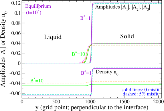
Figure 1: The equilibrium (solid/liquid coexistence) profile of the base state, for $\epsilon=0.02$, $B^{x}=1$ and $10$, and misfit $\varepsilon_{m}=0$ (solid lines) and $5\%$ (dashed lines).

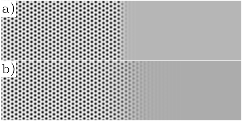
Figure 2: Sample equilibrium profiles of the complete density field $n$ as reconstructed from $n_{0}^{0}$ and $A_{j}^{0}$ for $\epsilon=0.02$, a misfit of $3\%$, and $B^{x}=1$ and $10$ in a) and b) respectively.

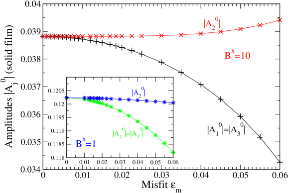
Figure 3: The equilibrium amplitudes $|A_{j}^{0}|$ in the solid region as a function of misfit $\varepsilon_{m}$, for $\epsilon=0.02$. The results in the main panel correspond to $B^{x}=10$, and those in the inset are for $B^{x}=1$. Note the much larger vertical scale in the inset.

The equilibrium profile for the base state (with solid/liquid coexistence) is given in Fig. 1, corresponding to non-growing, stationary films of different misfit strains $\varepsilon_{m}$ and elastic constants (as determined by $B^{x}$). The amplitudes and $n_{0}^{0}$ can be used to reconstruct the full density field $n$ via Eq. (4), as shown in Fig. 2. This figure highlights the increase in interfacial width as the magnitude of elastic moduli (i.e., $B^{x}$) increases. Since the stationary solution of Eqs. (15) and (16) cannot be obtained analytically, the results shown were obtained by numerical solutions based on a pseudospectral method. To apply the periodic boundary condition, we set the initial configuration as a pair of symmetric liquid-solid interfaces located at $y=L_{y}/4$ and $3L_{y}/4$ respectively, with $L_{y}$ the one-dimensional (1D) system size which is chosen up to $L_{y}=8192$ in our calculations so that these two interfaces are sufficiently far apart from each other and thus evolve independently. In the numerical algorithm adopted, the second order Crank-Nicholson time stepping scheme is used for the linear terms, while a second order Adams-Bashford explicit method is applied for the nonlinearities. A grid spacing $\Delta y=\lambda_{0}/8$ (i.e., 8 grid points per basic wavelength $\lambda_{0}=2\pi/q_{0}$) is chosen in most of calculations, although similar results have been obtained with much larger $\Delta y$. Relatively large time steps $\Delta t$ can be adopted without losing numerical stability: We use $\Delta t=0.5$ (or even $1$) for $B^{x}\geq 10$, and $\Delta t=0.2$ for $B^{x}=1$ with sharp interface. We also use the same algorithm and parameters in the stability/perturbation calculations given in Sec. IV.

For finite misfits the amplitudes $|A_{1}^{0}|=|A_{3}^{0}|\neq|A_{2}^{0}|$ and their difference increases with $\varepsilon_{m}$ as shown in Fig. 3. This corresponds to a triangular structure distorted along the $y$ direction (the surface normal) and the degree of distortion increases with misfit strain. Also as shown in Fig. 1, for larger value of $B^{x}$ which corresponds to smaller bulk modulus (as we calculate based on one-mode approximation; see Sec. IV), the interface or film surface is more diffuse (i.e., with larger interface width), but with a narrower coexistence region (i.e., smaller but nonzero miscibility gap). This can also be seen in Fig. 4, which shows the liquidus and solidus rescaled density $n_{0}^{\rm liq}$, $n_{0}^{\rm sol}$ as well as the miscibility gap $\Delta n_{0}=n_{0}^{\rm sol}-n_{0}^{\rm liq}$ as a function of misfit $\varepsilon_{m}$. The size of miscibility gap decreases with the increasing magnitude of misfit, and shows slight asymmetry with respect to the misfit sign as a result of different non-linear elastic effects on liquid-solid coexistence property for tensile and compressive strains.

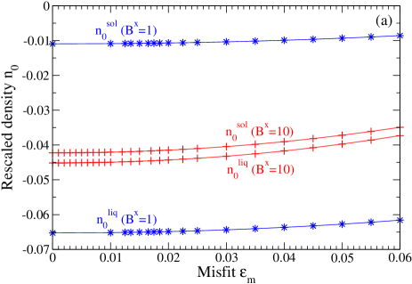
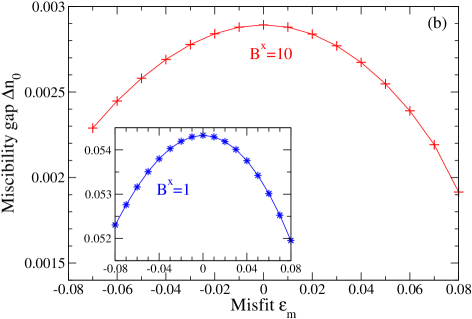
Figure 4: (a) The equilibrium densities $n_{0}^{\rm liq}$ and $n_{0}^{\rm sol}$ (in the coexisting liquid and solid regions respectively) as a function of misfit strain $\varepsilon_{m}$, with parameters the same as those of Fig. 3. (b) The size of miscibility gap $\Delta n_{0}=n_{0}^{\rm sol}-n_{0}^{\rm liq}$ as a function of $\varepsilon_{m}$, for $B^{x}=10$ (the main panel) and $1$ (the inset); Note the large vertical scale for $B^{x}=1$ in the inset.

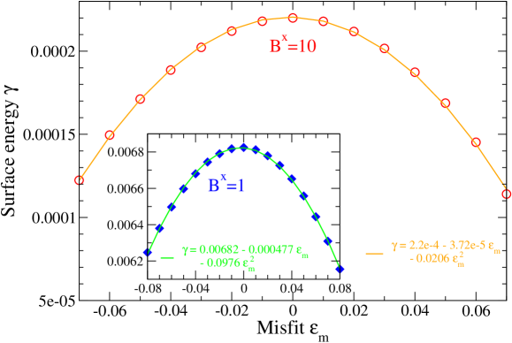
Figure 5: Results of surface tension $\gamma$ for different misfit strains $\varepsilon_{m}$, with parameters the same as those of Fig. 3. Also shown are the quadratic fitting results for $B^{x}=10$ (in the main panel) and $1$ (in the inset). Note that the vertical scale in the inset for $B^{x}=1$ is much larger.

We also calculate the surface tension $\gamma$ as a function of misfit strain since it is one of the important factors for determining film stability and island formation. Surface energy is known to play a stabilization role on film evolution and for simplicity is often approximated as misfit independent in many strained film studies. Srolovitz (1989); Spencer et al. (1991, 1993); Müller and Grant (1999); Kassner et al. (2001); Wise et al. (2005); Shilkrot et al. (2000); Huang and Desai (2003); Huang et al. (2003); Guyer and Voorhees (1995); Léonard and Desai (1998); Spencer et al. (2001); Huang and Desai (2002a, b) However in the presence of a strain field, the surface energy is known to vary as a result of intrinsic surface stress ${\bm{\sigma}}^{0}$ and is usually expanded up to 2nd order in terms of strain tensor $u_{ij}$ (with $i,j$ the film surface coordinate indices) in linear elasticity theory, Wolf (1993); Shchukin and Bimberg (1999) i.e.,

$$\gamma=\gamma_{0}+\sigma^{0}_{ij}u_{ij}+\frac{1}{2}S_{ijkl}u_{ij}u_{kl},$$ (17)

where $S_{ijkl}$ are the surface excess elastic moduli. Both $\sigma_{ij}^{0}$ and $S_{ijkl}$ can be either positive or negative. Shchukin and Bimberg (1999) For the 1D surface considered here, strain $u_{xx}=\varepsilon_{m}$ and hence Eq. (17) gives $\gamma=\gamma_{0}+\sigma^{0}_{xx}\varepsilon_{m}+S_{xxxx}\varepsilon_{m}^{2}/2$, which is consistent with our amplitude-equation calculations shown in Fig. 5. Data fitting of our numerical results yields $\gamma_{0}=6.82\times 10^{-3}$, $\sigma^{0}_{xx}=-4.77\times 10^{-4}$, $S_{xxxx}/2=-9.76\times 10^{-2}$ for $B^{x}=1$, and $\gamma_{0}=2.20\times 10^{-4}$, $\sigma^{0}_{xx}=-3.72\times 10^{-5}$, $S_{xxxx}/2=-2.06\times 10^{-2}$ for $B^{x}=10$ (all in dimensionless unit), showing smaller surface energy for larger value of $B^{x}$ (with larger surface width). These results indicate that for the parameters chosen, both the intrinsic surface stress $\sigma^{0}_{xx}$ and excess elastic moduli $S_{xxxx}$ are negative, leading to the decrease of surface energy with increasing magnitude of misfit strain. In addition the tensile surface stress is rather weak which can explain the weak asymmetry of $\gamma$ between tensile and compressive strained films.

IV Morphological Instability and Island Scaling

For strained films with nonzero misfit, a morphological instability of film surface is known to develop as a result of strain energy relaxation, leading to surface undulations and then the formation of surface nanostructures such as strained islands. Such an instability can be revealed via a linear analysis of amplitude equations given above. We can expand the amplitudes in Fourier series as

$$A_{j}^{\prime}(x,y,t)=A_{j}^{0}(y)+\sum\limits_{q_{x}}\hat{A}_{j}(q_{x},y,t)e^{iq_{x}x},$$ (18)

$$n_{0}(x,y,t)=n_{0}^{0}(y)+\sum\limits_{q_{x}}\hat{n}_{0}(q_{x},y,t)e^{iq_{x}x},$$ (19)

where $A_{j}^{0}(y)$ and $n_{0}^{0}(y)$ are the planar base solutions discussed in the previous section and the perturbed quantities $\hat{A}_{j}$ and $\hat{n}_{0}$ obey the following linearized equations,

$$\partial_{t}\hat{A}_{1}(q_{x},y,t) =-q_{0}^{2}\left\{\left[-\epsilon+3{n_{0}^{0}}^{2}-2gn_{0}^{0}+\left(\partial_{y}^{2}-i(q_{0}+\delta_{y})\partial_{y}-q_{x}^{2}+(\sqrt{3}q_{0}+2\delta_{x})q_{x}\right.\right.\right.$$ (23)

$$\left.\left.-\sqrt{3}q_{0}\delta_{x}-\delta_{x}^{2}-q_{0}\delta_{y}/2-\delta_{y}^{2}/4\right)^{2}+6\left(|A_{1}^{0}|^{2}+|A_{2}^{0}|^{2}+|A_{3}^{0}|^{2}\right)\right]\hat{A}_{1}(q_{x},y,t)$$

$$+6A_{1}^{0}\left[{A_{2}^{0}}^{*}\hat{A}_{2}(q_{x},y,t)+{A_{3}^{0}}^{*}\hat{A}_{3}(q_{x},y,t)\right]+3{A_{1}^{0}}^{2}\hat{A}_{1}^{*}(-q_{x},y,t)$$

$$+\left[(6n_{0}^{0}-2g){A_{3}^{0}}^{*}+6A_{1}^{0}A_{2}^{0}\right]\hat{A}_{2}^{*}(-q_{x},y,t)$$

$$+\left[(6n_{0}^{0}-2g){A_{2}^{0}}^{*}+6A_{1}^{0}A_{3}^{0}\right]\hat{A}_{3}^{*}(-q_{x},y,t)$$

$$\left.+\left[(6n_{0}^{0}-2g)A_{1}^{0}+6{A_{2}^{0}}^{*}{A_{3}^{0}}^{*}\right]\hat{n}_{0}(q_{x},y,t)\right\},$$

$$\partial_{t}\hat{A}_{2}(q_{x},y,t) =-q_{0}^{2}\left\{\left[-\epsilon+3{n_{0}^{0}}^{2}-2gn_{0}^{0}+\left(\partial_{y}^{2}+2i(q_{0}+\delta_{y})\partial_{y}-q_{x}^{2}\right.\right.\right.$$

$$\left.\left.-2q_{0}\delta_{y}-\delta_{y}^{2}\right)^{2}+6\left(|A_{1}^{0}|^{2}+|A_{2}^{0}|^{2}+|A_{3}^{0}|^{2}\right)\right]\hat{A}_{2}(q_{x},y,t)$$

$$+6A_{2}^{0}\left[{A_{1}^{0}}^{*}\hat{A}_{1}(q_{x},y,t)+{A_{3}^{0}}^{*}\hat{A}_{3}(q_{x},y,t)\right]+3{A_{2}^{0}}^{2}\hat{A}_{2}^{*}(-q_{x},y,t)$$

$$+\left[(6n_{0}^{0}-2g){A_{3}^{0}}^{*}+6A_{1}^{0}A_{2}^{0}\right]\hat{A}_{1}^{*}(-q_{x},y,t)$$

$$+\left[(6n_{0}^{0}-2g){A_{1}^{0}}^{*}+6A_{2}^{0}A_{3}^{0}\right]\hat{A}_{3}^{*}(-q_{x},y,t)$$

$$\left.+\left[(6n_{0}^{0}-2g)A_{2}^{0}+6{A_{1}^{0}}^{*}{A_{3}^{0}}^{*}\right]\hat{n}_{0}(q_{x},y,t)\right\},$$

$$\partial_{t}\hat{A}_{3}(q_{x},y,t) =-q_{0}^{2}\left\{\left[-\epsilon+3{n_{0}^{0}}^{2}-2gn_{0}^{0}+\left(\partial_{y}^{2}-i(q_{0}+\delta_{y})\partial_{y}-q_{x}^{2}-(\sqrt{3}q_{0}+2\delta_{x})q_{x}\right.\right.\right.$$

$$\left.\left.-\sqrt{3}q_{0}\delta_{x}-\delta_{x}^{2}-q_{0}\delta_{y}/2-\delta_{y}^{2}/4\right)^{2}+6\left(|A_{1}^{0}|^{2}+|A_{2}^{0}|^{2}+|A_{3}^{0}|^{2}\right)\right]\hat{A}_{3}(q_{x},y,t)$$

$$+6A_{3}^{0}\left[{A_{1}^{0}}^{*}\hat{A}_{1}(q_{x},y,t)+{A_{2}^{0}}^{*}\hat{A}_{2}(q_{x},y,t)\right]+3{A_{3}^{0}}^{2}\hat{A}_{3}^{*}(-q_{x},y,t)$$

$$+\left[(6n_{0}^{0}-2g){A_{2}^{0}}^{*}+6A_{1}^{0}A_{3}^{0}\right]\hat{A}_{1}^{*}(-q_{x},y,t)$$

$$+\left[(6n_{0}^{0}-2g){A_{1}^{0}}^{*}+6A_{2}^{0}A_{3}^{0}\right]\hat{A}_{2}^{*}(-q_{x},y,t)$$

$$\left.+\left[(6n_{0}^{0}-2g)A_{3}^{0}+6{A_{1}^{0}}^{*}{A_{2}^{0}}^{*}\right]\hat{n}_{0}(q_{x},y,t)\right\},$$

$$\partial_{t}\hat{n}_{0}(q_{x},y,t) =\left(\partial_{y}^{2}-q_{x}^{2}\right)\left\{\left[-\epsilon+3{n_{0}^{0}}^{2}-2gn_{0}^{0}+\left(\partial_{y}^{2}-q_{x}^{2}+q_{0}^{2}\right)^{2}\right.\right.$$

$$\left.+6\left(|A_{1}^{0}|^{2}+|A_{2}^{0}|^{2}+|A_{3}^{0}|^{2}\right)\right]\hat{n}_{0}(q_{x},y,t)$$

$$+\left[(6n_{0}^{0}-2g){A_{1}^{0}}^{*}+6A_{2}^{0}A_{3}^{0}\right]\hat{A}_{1}(q_{x},y,t)$$

$$+\left[(6n_{0}^{0}-2g){A_{2}^{0}}^{*}+6A_{1}^{0}A_{3}^{0}\right]\hat{A}_{2}(q_{x},y,t)$$

$$+\left[(6n_{0}^{0}-2g){A_{3}^{0}}^{*}+6A_{1}^{0}A_{2}^{0}\right]\hat{A}_{3}(q_{x},y,t)$$

$$+\left[(6n_{0}^{0}-2g)A_{1}^{0}+6{A_{2}^{0}}^{*}{A_{3}^{0}}^{*}\right]\hat{A}_{1}^{*}(-q_{x},y,t)$$

$$+\left[(6n_{0}^{0}-2g)A_{2}^{0}+6{A_{1}^{0}}^{*}{A_{3}^{0}}^{*}\right]\hat{A}_{2}^{*}(-q_{x},y,t)$$

$$\left.+\left[(6n_{0}^{0}-2g)A_{3}^{0}+6{A_{1}^{0}}^{*}{A_{2}^{0}}^{*}\right]\hat{A}_{3}^{*}(-q_{x},y,t)\right\}.$$

The stability of the base planar film surface is examined by introducing initial small random perturbations into $\hat{A}_{j}$ and $\hat{n}_{0}$, and solving numerically the initial value problem defined by Eqs. (23)–(23), given a specific value of $q_{x}$. The numerical algorithm introduced in Sec. III is employed, with the use of a pseudospectral method and periodic boundary conditions.

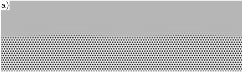
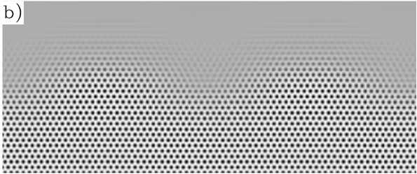
Figure 6: Reconstruction of full density field $n$ for an interface profile showing island formation, with a $3\%$ misfit at $\epsilon=0.02$. a) corresponds to density $n$ at $t=125,000$, for $B^{x}=1$ and the maximum instability wave number $q_{x}=0.0184$, while b) corresponds to $n$ at $t=2000$, for $B^{x}=10$ and $q_{x}=0.026$.

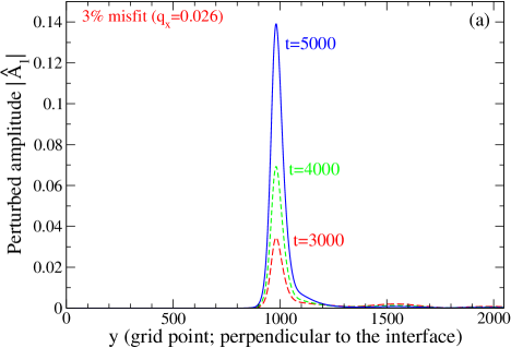
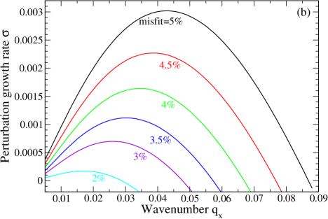
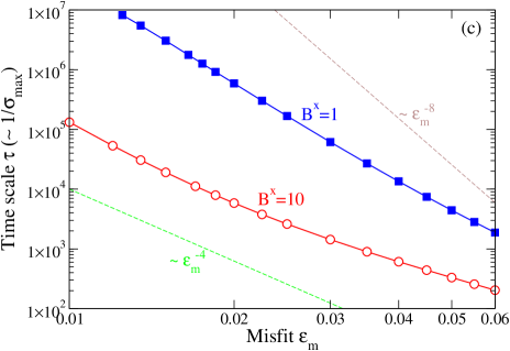
Figure 7: (a) Amplitude perturbations, which grow with time around the solid/liquid interface for $\epsilon=0.02$, $B^{x}=10$, wave number $q_{x}=0.026$ and $3\%$ misfit. (b) Perturbation growth rate $\sigma$ as a function of wave number $q_{x}$, for different values of misfit $\varepsilon_{m}$. Other parameters are the same as (a). (c) Characteristic time scale $\tau$ ($\sim 1/\sigma_{\rm max}$) for the mounding instability as a function of misfit $\varepsilon_{m}$, for $B^{x}=1$ and $10$. Two power laws, $\tau\sim\varepsilon_{m}^{-8}$ and $\sim\varepsilon_{m}^{-4}$, are also shown for comparison.

For nonzero misfit, within a certain range of wave number $q_{x}$ the initial perturbations of $\hat{A}_{j}$ and $\hat{n}_{0}$ grow with time around the liquid-solid interface, while they always decay to zero far from the interface region, showing the stability of both the solid and liquid bulks. This interface instability results in the formation of islands or mounds at the liquid-solid interface, as shown in Fig. 6. This figure was obtained by reconstructing full density field $n$ from the amplitudes with wave number $q_{x}$ of maximum instability (based on Eq. (4)). A typical example of the dynamics of the amplitudes that gives rise to this instability is given in Fig. 7a. We then calculate the perturbation growth rate $\sigma(q_{x})$, noting that $|\hat{A}_{j}|,|\hat{n}_{0}|\propto e^{\sigma t}$. This process is repeated for a range of perturbation wave number $q_{x}$, and also for various misfits $\varepsilon_{m}$. Some results of the dispersion relation are shown in Fig. 7b, for $\epsilon=0.02$ and $B^{x}=10$. Previous work of continuum elasticity or phase-field theory has predicted various forms of dispersion relation, including $\sigma\simeq\alpha_{3}q^{3}-\alpha_{4}q^{4}$ (for surface-diffusion dominated process, Srolovitz (1989); Spencer et al. (1991, 1993)) $\sigma\simeq-\alpha_{2}q^{2}+\alpha_{3}q^{3}-\alpha_{4}q^{4}$ (if considering wetting effects, Levine et al. (2007); Eisenberg and Kandel (2000)) $\sigma\simeq\alpha_{1}q-\alpha_{2}q^{2}$ (in the case of evaporation-condensation, Srolovitz (1989); Müller and Grant (1999); Kassner et al. (2001)) or $\sigma\simeq\alpha_{2}q^{2}-\alpha_{3}q^{3}$ (for bulk-diffusion dominated case, Wu and Voorhees (2009)) with $q$ the wave number and $\alpha_{i}$ ($i=1,...,4$) the model-dependent coefficients that are usually a function of surface tension and elastic moduli. However, none of these forms fits our dispersion data, which instead can be well fitted only by a 4th order polynomial of $q_{x}$ for all range of wave numbers, similar to a combination of all the above forms. This is not unexpected, given that all factors of surface diffusion, bulk diffusion, wetting effects, and evaporation/condensation are naturally incorporated in the PFC model and cannot be easily decoupled. This can be seen through the fact that the PFC modeling of epitaxial growth involves the coexistence of liquid-solid interface that buckles and evolves, and thus naturally involves the diffusion processes along the interface and between liquid region and solid film, and also the variation of material properties such as surface/interface energy and elastic relaxation across the interface (i.e., the wetting effects). We expect that an important parameter controlling these different processes would be $\epsilon$, the temperature distance from the melting point. The $\epsilon$ (or temperature) dependence of properties of system relaxation has been known for pattern formation systems, and is also seen in our PFC studies. Here we focus on high temperature regime where the amplitude equation representation is most relevant and effective, and hence choose $\epsilon=0.02$ which is different from other studies with larger $\epsilon$ and hence lower growth temperature (e.g., $\epsilon=0.1$ in Ref. Wu and Voorhees, 2009). For such small $\epsilon$ (high temperature) surface diffusion process is more prominent and coupled with the bulk diffusion process, a phenomenon that might be weakened or absent in low temperature growth (e.g., in Ref. Wu and Voorhees, 2009 only bulk diffusion behavior has been identified in the dispersion relation obtained from the original PFC equation).

The development of surface perturbations and instability can be characterized by an evolution time scale $\tau$, which can be approximated via the inverse of maximum perturbation growth rate $\sigma_{\rm max}$ and is found to scale as $\varepsilon_{m}^{-8}$ or $\varepsilon_{m}^{-4}$ in continuum elasticity theory with the assumed mass transport mechanism dominated by surface diffusion or evaporation-condensation respectively. Srolovitz (1989); Spencer et al. (1993) However, our calculations yield results more complicated than this single power law behavior, as shown in Fig. 7c, which can also be expected from the coupling of various mass transport processes in this modeling as discussed above. Our results show that the time scale $\tau$ decreases with misfit strain $\varepsilon_{m}$, since the $\varepsilon_{m}$ provides the driving force for the morphological instability. $\tau$ is also found to significantly decreases when $B^{x}$ increases. For example at a given misfit, $\tau$ is typically one or two orders of magnitude larger for $B^{x}=1$ compared with $B^{x}=10$. This difference is most likely due to the significant decrease in surface energy and increase in interfacial thickness as $B^{x}$ is increased, as shown in Fig. 5 and Fig. 1 respectively.

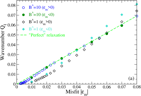
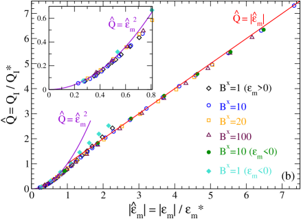
Figure 8: (a) Characteristic wave number $Q_{I}$ of film surface instability as a function of misfit strain magnitude $|\varepsilon_{m}|$, for different values of $B^{x}=1$ and $10$ and both compressive ($\varepsilon_{m}>0$) and tensile ($\varepsilon_{m}<0$) films. The limit imposed by “perfect” relaxation condition is indicated by a dashed line. (b) Scaling of island wave number based on a crossover wave number $Q^{*}=3\gamma q_{0}^{2}/4E$ and misfit $\varepsilon_{m}^{*}=3\gamma q_{0}/4E$, for different values of $B^{x}$ which is proportional to film elastic modulus. The inset highlights the crossover to the continuum result of $Q_{I}\sim\varepsilon_{m}^{2}$ at small misfit limit.

The maximum of the growth rate determines the characteristic wave number $Q_{I}$ for the instability, and hence the characteristic wave number of the island/mound formation on the film surface. We plot in Fig. 8a the relation of this instability/island wave number $Q_{I}$ vs. misfit strain $\varepsilon_{m}$, for different values of $B^{x}$ and for both compressive ($\varepsilon_{m}>0$) and tensile ($\varepsilon_{m}<0$) films. For each value of $B^{x}$ we can identify two regions, corresponding to a quadratic behavior of $Q_{I}\sim\varepsilon_{m}^{2}$ at small misfits (see also the inset of Fig. 8b) and a linear dependence of $Q_{I}$ on $\varepsilon_{m}$ for large enough strains. Such quadratic scaling in the small misfit limit is consistent with the well-known results of continuum theory including all different assumptions of dominant mechanisms such as surface diffusion, evaporation-condensation and wetting effects. Srolovitz (1989); Spencer et al. (1991, 1993); Spencer and Blanariu (2005); Levine et al. (2007); Eisenberg and Kandel (2000) However, this $\varepsilon_{m}^{2}$ scaling result differs from the experimental findings in SiGe/Si(001) growth, Sutter and Lagally (2000); Tromp et al. (2000) which indicate the linear behavior $Q_{I}\sim\varepsilon_{m}$ for the stress-driven surface instability and coherent epitaxial islands. Although this observation of a linear relationship is qualitatively similar to what we obtain above for large enough misfits, it should be cautioned that the experimental systems involve more complicated factors related to the SiGe alloying nature that is not considered here, particularly the atomic mobility difference between the two film components which was verified by recent first principle calculations Huang et al. (2006) and was believed to play a key role on island size scaling. Tersoff (2000); Spencer et al. (2001)

For the single-component films studied here the crossover from the quadratic scaling at the continuum weak-strain limit to linear behavior at high strains is most likely due to the discrete nature of the crystalline lattice that is implicitly included in the amplitude formulation. It is known (and verified in direct simulations of PFC Eq. (3) Elder and Grant (2004); Elder et al. (2007); Huang and Elder (2008)) that at late times the instability to form islands or mounds leads to the nucleation of dislocations around the edges of islands or in the valleys between the mounds. These dislocations nucleate to relieve strain in the film and appear at earlier times for larger misfit strains. Here we define a length scale, $\lambda_{R}$, for “perfect” relaxation such that if the dislocations nucleate at this distance apart, strain in the film will be completely relieved (aside from the strain induced by the dislocations themselves). We can then make the assumption that if the continuum prediction for most unstable wavelength is smaller than $\lambda_{R}$, continuum theory will break down. To evaluate $\lambda_{R}$ consider a 1+1 dimensional film; assume $L_{x}$ being the lateral length of film surface and by definition we have $L_{x}=Na=Ma_{0}$, where $N$ is the number of atoms in strained lattice, $M$ is the atom number for unstrained state after dislocations nucleate, and $a$ and $a_{0}$ are the corresponding lattice constants already defined in Eq. (9). Thus from Eq. (9) for the definition of misfit, we obtain $\varepsilon_{m}=(N-M)/M$, leading to the average distance between dislocations $\lambda_{R}=L/|N-M|=L/(M|\varepsilon_{m}|)=a_{0}/|\varepsilon_{m}|$, with the associated wave number $Q_{R}=q_{x0}|\varepsilon_{m}|$ (plotted as a dashed line in Fig. 8a). Assuming that on average at least one dislocation will appear at each island edge/valley, this wave number $Q_{R}$ will then be the upper limit imposed by the discrete nature of the lattice, as it would be unphysical for islands with size smaller than $\lambda_{R}$ to appear which would instead cause the “overrelaxation” of the film lattice. Our results of island wave number $Q_{I}$ for different values of $B^{x}$ ($=10,20,100$) all converge to this limit at large misfit strains (except for $B^{x}=1$ which will be discussed below).

This “perfect” relaxation condition is expected to be met at large enough misfits, but not at small strains where dislocations appear at far late stage after islands form, leading to the crossover phenomenon between two scaling regimes given in Fig. 8. This crossover occurs when $Q_{I}({\rm of~{}small~{}misfit~{}limit})=Q_{R}$. As stated above, at small $\varepsilon_{m}$ we can recover the result of continuum theory which predicts $Q_{I}\propto(E/\gamma)\varepsilon_{m}^{2}$ (with $E$ the Young’s modulus). Srolovitz (1989); Spencer et al. (1991, 1993) In our calculations based on the PFC model and amplitude equations, we evaluate $E$ from a one-mode approximation, Elder and Grant (2004); Elder et al. (2007) $E=B^{x}A_{\rm min}^{2}/2$, where $A_{\rm min}=4(g-3n_{0}+\sqrt{g^{2}+24n_{0}g-36n_{0}^{2}+15\varepsilon_{m}})/15$. Using the results of $\gamma$ given in Sec. III, we can fit the small misfit data well into a form $Q_{I}=4E\varepsilon_{m}^{2}/3\gamma$ (for all values of $B^{x}$; see the inset of Fig. 8b). Therefore, the misfit ($\varepsilon_{m}^{*}$) and island wave number ($Q_{I}^{*}$) at the crossover can be determined via $Q_{I}^{*}=4E{\varepsilon_{m}^{*}}^{2}/3\gamma=Q_{R}=q_{x0}\varepsilon_{m}^{*}$, resulting in $\varepsilon_{m}^{*}=3\gamma q_{x0}/4E$ and $Q_{I}^{*}=3\gamma q_{x0}^{2}/4E$. Defining rescaled quantities $\hat{Q}=Q_{I}/Q_{I}^{*}$ and $\hat{\varepsilon}_{m}=\varepsilon_{m}/\varepsilon_{m}^{*}$, we can then scale all the data from different conditions (e.g., films of different elastic constants, for $B^{x}>1$) onto a single universal scaling curve accommodating all range of misfit strains, for both compressive and tensile films (see Fig. 8b). The crossover misfit strain $\varepsilon_{m}^{*}$ can be very small ($<2\%$, depending on e.g., film elastic properties), showing the breakdown of continuum approach even at relatively large scales.

Note that although this linear behavior due to “perfect” lattice relaxation and the scaling crossover have been observed in our previous work, Huang and Elder (2008) it was limited to compressive strained films and not-too-large misfits. However, the more generalized study given here shows a small deviation from the limit of “perfect” relaxation for small value of $B^{x}$, as indicated in Fig. 8a with island wave numbers of $B^{x}=1$ lying above such upper limit (the dashed line) when the magnitude of mismatch $|\varepsilon_{m}|$ exceeds $5\%$ (for tensile films) or $6\%$ (compressive). Similar deviation can be seen in the corresponding scaling plot of Fig. 8b. Nevertheless, at large misfits the linear scaling behavior is still maintained, which is qualitatively different from the quadratic scaling at the small strain limit. Based on the discussions given above for “perfect” relaxation condition, it is expected that $Q_{I}>Q_{R}$ occurs only when some of the island edges would be dislocation-free even at late evolution times. The condition for this scenario is not clear; but our results suggest that this may occur when the liquid-solid interface (or film surface) is sharp enough. As given in Fig. 9, the interface width $W$ decreases with the value of $B^{x}$, and is particularly small at $B^{x}=1$ (with $W\sim 13.5\Delta y$ for both tensile and compressive films, less than 2 lattice spacing) as compared to others. It could then be expected that details of film morphological evolution, including instability and island formation, would be different for such sharp interface, as somewhat indicated in Fig. 8. Further studies are needed to clarify this special scenario of strained film evolution.

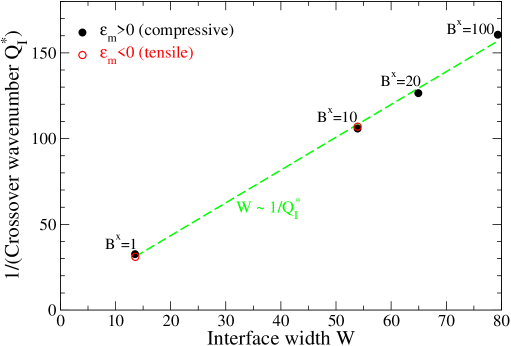
Figure 9: The linear relation between the liquid-solid interface width $W$ and the inverse of crossover wave number $1/Q_{I}^{*}$, for $\epsilon=0.02$ and both compressive (filled symbols) and tensile (open symbols) films. Values of $B^{x}$ are also indicated on the plot.

Fig. 9 also yields the effect of finite interface width $W$ on the island size (or wave number) scaling. We find $1/Q_{I}^{*}\sim W$, i.e., a linear relation between crossover instability wavelength ($=2\pi/Q_{I}^{*}$) and the interface thickness. This is consistent with most recent results of direct PFC simulations Wu and Voorhees (2009) which indicate that the discrepancy or crossover between the classical elasticity result of quadratic scaling of $Q_{I}$ and the linear behavior identified in the PFC modeling could be attributed to the finite thickness of the interface, a fact that is neglected in the classical continuum theory. As seen in Fig. 9, when $W\rightarrow 0$ (i.e., the assumption adopted in continuum elasticity theory), we have $Q_{I}^{*}\rightarrow\infty$ and hence recover the continuum theory prediction of $Q_{I}\sim\varepsilon_{m}^{2}$ for the whole range of misfit strain, as expected. Corresponding to real experimental systems, Fig. 9 predicts that at constant growth temperature (same $\epsilon$ value), the liquid-solid interface thickness varies with film elastic modulus (or the value of $B^{x}$), and for different film materials the crossover island size separating two island scaling regimes increases linearly with the interface thickness.

Another important feature of our results is the asymmetry between tensile and compressive films which, however, becomes distinct only at small enough $B^{x}$ and large enough misfits (see Fig. 8 for the data of $B^{x}=1$). Given the important role played by the surface energy $\gamma$ on film stability and evolution, we expect this asymmetric phenomenon of island wave number to be closely related to the property of $\gamma$ shown in Fig. 5. The intrinsic surface stress $\sigma_{xx}^{0}$ determined for $B^{x}=1$ is an order of magnitude larger than that for $B^{x}=10$, leading to much larger value of surface energy difference between tensile and compressive strains; also such difference increases with the magnitude of misfit strain. The corresponding behavior of surface instability and island formation would then follow the similar trend, as observed in Fig. 8.

V Free Energy Analysis and Mode Coupling

To further elucidate the properties of the strained surface, it is interesting to analyze the effective free energy ${\cal F}$ (given in Eq. (8)). Consider the net change of ${\cal F}$ relative to that of a planar interface, i.e.,

$$\Delta{\cal F}={\cal F}-{\cal F}^{0},$$ (24)

where ${\cal F}^{0}$ is the free energy of the planar interface given in Eq. (16). $\Delta{\cal F}<0$ indicates film surface instability against the initial perturbation, while $\Delta{\cal F}>0$ refers to the energy penalty of any perturbations and hence corresponds to stability of planar film surface.

Based on the Fourier expansion (18) and (19), $\Delta{\cal F}$ can be expanded up to second order in the perturbed quantities $\hat{A}_{j}$ and $\hat{n}_{0}$, i.e.,

$$\Delta{\cal F}=\Delta{\cal F}^{(1)}+\Delta{\cal F}^{(2)}.$$ (25)

Detailed expression of the first order term $\Delta{\cal F}^{(1)}$ is given in the Appendix (see Eq. (28)). We find numerically $\Delta{\cal F}^{(1)}\sim 0$, and hence the net energy change $\Delta{\cal F}$ is determined by the second order quantity

$$\Delta{\cal F}^{(2)}=\Delta{\cal F}_{+}+\Delta{\cal F}_{-},$$ (26)

where

$$\Delta{\cal F}_{-}=L_{x}\int dy\sum\limits_{q_{x}}\left\{(6n_{0}^{0}-2g)\sum\limits_{j=1}^{3}\left[A_{j}^{0}\hat{A}_{j}^{*}(-q_{x})+{A_{j}^{0}}^{*}\hat{A}_{j}(q_{x})\right]\hat{n}_{0}^{*}(q_{x})\right.$$

$$\left.+(6n_{0}^{0}-2g)\left[A_{3}^{0}\hat{A}_{1}(q_{x})\hat{A}_{2}(-q_{x})+A_{2}^{0}\hat{A}_{1}(q_{x})\hat{A}_{3}(-q_{x})+A_{1}^{0}\hat{A}_{2}(q_{x})\hat{A}_{3}(-q_{x})+{\rm c.c.}\right]\right\},$$

(27)

with $\hat{A}_{j}(q_{x})=\hat{A}_{j}(q_{x},y,t)$ and $\hat{n}_{0}(q_{x})=\hat{n}_{0}(q_{x},y,t)$, and the contribution $\Delta{\cal F}_{+}$ is shown in Eq. (A) of the Appendix.

Figure 10: Time evolution of effective free energy density change $\Delta{\cal F}$ (per unit volume $V=L_{x}L_{y}$) of the perturbed state, with misfit $\varepsilon_{m}=3\%$, wave number $Q_{I}=0.026$, $\epsilon=0.02$, and $B^{x}=10$. Also included are the positive contribution $\Delta{\cal F}_{+}$ and the negative contribution $\Delta{\cal F}_{-}$.

Given the numerical solution for the perturbed amplitudes (see Eqs. (23)–(23)) as described in Sec. IV, $\Delta{\cal F}$ ($\simeq\Delta{\cal F}^{(2)}$) can be approximated via the most unstable characteristic wave number by substituting the numerical solutions for amplitudes at $q_{x}=\pm Q_{I}$. We find that all terms in Eq. (A) are positive, i.e., $\Delta{\cal F}_{+}>0$; both two terms in Eq. (27) yield negative contribution (noting that usually $6n_{0}^{0}-2g<0$ for liquid-solid coexistence), so that $\Delta{\cal F}_{-}<0$, and the magnitude of the last term is much larger than the 1st one. As shown in Fig. 10, at large enough time $\Delta{\cal F}_{-}$ dominates over the stabilizing terms in $\Delta{\cal F}_{+}$, leading to negative net free energy change $\Delta{\cal F}$ and thus the film instability. Note that the last term in Eq. (27), which dominates $\Delta{\cal F}_{-}$, arises from the 2nd-order expansion of $(A_{1}A_{2}A_{3}+A_{1}^{*}A_{2}^{*}A_{3}^{*})$ in the effective free energy formula (8). It represents the coupling of different modes of complex amplitudes, and our numerical results show that it contributes to the integral of $\Delta{\cal F}_{-}$ only in the interface or film surface region (as the perturbed amplitudes decay fast in the bulks). We can then argue that it is the mode coupling of complex amplitudes at the liquid-solid interface that is mainly responsible for the morphological instability of the strained film. Note that the amplitudes of structural profile $A_{j}$ are complex, and thus their evolution involves an important process of phase perturbation (or phase winding). Physically this phase behavior corresponds to the elastic relaxation of the lattice structure, and thus the mode coupling property identified above indicates that the coupling of elastic relaxation for different lattice modes (or wave vectors) around the film surface would be one of the major factors underlying the film instability and mounding behavior. Such phase behavior is related to details of crystalline structure, as captured by the PFC model and the amplitude equation formalism, but not by the continuum theory. Furthermore, the competition between $\Delta{\cal F}_{+}$ ($>0$) and $\Delta{\cal F}_{-}$ ($<0$) shown in Fig. 10 is consistent with previous analysis of continuum elasticity theory showing the competition between film stabilization effects (such as surface energy) and destabilizing factors (mainly elastic effects). Srolovitz (1989); Spencer et al. (1991, 1993); Guyer and Voorhees (1995); Léonard and Desai (1998); Spencer et al. (2001); Huang and Desai (2002a, b) Note also that the above mechanism identified should be already incorporated in the original PFC equation (3) and the associated PFC free energy (1), while the analysis given here based on the amplitude formulation has the advantage of being able to single out individual contributions from different lattice modes.

VI Conclusions

We have investigated the detailed properties of a strained film surface, its morphological instability, and the associated island wave number scaling through a systematic analysis of the amplitude equation formalism based on the phase field crystal model. We identify the amplitude and average density profiles of liquid-film coexisting interface, the interface width, miscibility gap, and surface energy (including intrinsic surface stress and excess elastic modulus), for various misfit strains (both magnitude and sign) and film elastic constants (or values of $B^{x}$). The morphological or mounding instability of the strained film is systematically examined, showing results absent in all previous continuum elasticity and phase-field approaches and atomistic modeling. In particular, we obtain a crossover phenomenon of instability or island wave number scaling, from the well-known continuum, ATG result of $Q_{I}\sim\varepsilon_{m}^{2}$ to a linear behavior $Q_{I}\sim\varepsilon_{m}$ at large enough strains which is identified by an upper limit imposed by the condition of “perfect” lattice relaxation. Most data (of different parameter ranges) can be scaled onto a universal scaling relation for the whole range of misfit strain, with some small deviations for very narrow liquid-solid interfaces in the large strain limit. The asymmetry of film properties between tensile and compressive strains is also observed. Note that although either linear or quadratic scaling has been reported in experiments (such as SiGe/Si(001)) and model simulations (e.g., kinetic MC) or continuum theory (e.g., ATG instability), the universal scaling relation with crossover of the two regions has not been found before. We expect our prediction here to be examined by experiments of single-component film epitaxy or atomistic simulations with large enough length and time scales.

Our study highlights an important feature of the amplitude formulation for strained film epitaxy, in that it can simultaneously reproduce continuum results (e.g., the ATG instability) and reveal significant corrections due to the microscopic nature of the crystalline structure. Our approach adopts a mesoscopic-level description of the system, via the amplitudes or envelopes of the slowly varying surface profile for which the well-developed continuum, mesoscopic theory can be applied. On the other hand, the crystalline nature of the strained film is preserved particularly via phase perturbations of the complex amplitudes that are prominent around the film surface. The latter has been emphasized through revealing the breakdown of traditional continuum approaches even at relatively small misfit stress and the associated crossover effect of island size scaling, and also through examining the origin of film instability that is accompanied by mode coupling of complex amplitudes in the liquid-solid interface region. Our results thus emphasize the importance of multiple scale modeling of complex material systems such as the strained film epitaxy process studied above. Note that although in this paper we focus on 2D hexagonal/triangular crystal structure, we expect the approach and analysis technique developed here to be directly extended for other crystalline symmetries and other surface directions, such as the epitaxial growth and island formation in 3D bcc or fcc films for which we have developed the corresponding amplitude expansion formulation very recently. Elder et al. (2010)

Appendix A Free energy expansion

In this appendix the detailed expansion forms of free energy difference $\Delta{\cal F}$ are presented. For the first order term $\Delta{\cal F}^{(1)}$ shown in Eq. (25), we have

$$\Delta{\cal F}^{(1)} =L_{x}\int dy\left\{\sum_{j=1}^{3}\left(-\epsilon+3{n_{0}^{0}}^{2}-2gn_{0}^{0}+3|A_{j}^{0}|^{2}\right)\left({A_{j}^{0}}^{*}\hat{A}_{j}(0)+{\rm c.c.}\right)\right.$$ (28)

$$+(6n_{0}^{0}-2g)\sum_{j=1}^{3}|A_{j}^{0}|^{2}\hat{n}_{0}(0)$$

$$+\left[\left(\partial_{y}^{2}+i(q_{0}+\delta_{y})\partial_{y}-\sqrt{3}q_{0}\delta_{x}-\delta_{x}^{2}-q_{0}\delta_{y}/2-\delta_{y}^{2}/4\right){A_{1}^{0}}^{*}\right]$$

$$\times\left[\left(\partial_{y}^{2}-i(q_{0}+\delta_{y})\partial_{y}-\sqrt{3}q_{0}\delta_{x}-\delta_{x}^{2}-q_{0}\delta_{y}/2-\delta_{y}^{2}/4\right)\hat{A}_{1}(0)\right]+{\rm c.c.}$$

$$+\left[\left(\partial_{y}^{2}-2i(q_{0}+\delta_{y})\partial_{y}-2q_{0}\delta_{y}-\delta_{y}^{2}\right){A_{2}^{0}}^{*}\right]$$

$$\times\left[\left(\partial_{y}^{2}+2i(q_{0}+\delta_{y})\partial_{y}-2q_{0}\delta_{y}-\delta_{y}^{2}\right)\hat{A}_{2}(0)\right]+{\rm c.c.}$$

$$+\left[\left(\partial_{y}^{2}+i(q_{0}+\delta_{y})\partial_{y}-\sqrt{3}q_{0}\delta_{x}-\delta_{x}^{2}-q_{0}\delta_{y}/2-\delta_{y}^{2}/4\right){A_{3}^{0}}^{*}\right]$$

$$\times\left[\left(\partial_{y}^{2}-i(q_{0}+\delta_{y})\partial_{y}-\sqrt{3}q_{0}\delta_{x}-\delta_{x}^{2}-q_{0}\delta_{y}/2-\delta_{y}^{2}/4\right)\hat{A}_{3}(0)\right]+{\rm c.c.}$$

$$+(6n_{0}^{0}-2g)\left[A_{2}^{0}A_{3}^{0}\hat{A}_{1}(0)+A_{1}^{0}A_{3}^{0}\hat{A}_{2}(0)+A_{1}^{0}A_{2}^{0}\hat{A}_{3}(0)+{\rm c.c.}\right]$$

$$+6\left(A_{1}^{0}A_{2}^{0}A_{3}^{0}+{A_{1}^{0}}^{*}{A_{2}^{0}}^{*}{A_{3}^{0}}^{*}\right)\hat{n}_{0}(0)+6\left(|A_{2}^{0}|^{2}+|A_{3}^{0}|^{2}\right)\left({A_{1}^{0}}^{*}\hat{A}_{1}(0)+{\rm c.c.}\right)$$

$$+6\left(|A_{1}^{0}|^{2}+|A_{3}^{0}|^{2}\right)\left({A_{2}^{0}}^{*}\hat{A}_{2}(0)+{\rm c.c.}\right)+6\left(|A_{1}^{0}|^{2}+|A_{2}^{0}|^{2}\right)\left({A_{3}^{0}}^{*}\hat{A}_{3}(0)+{\rm c.c.}\right)$$

$$\left.+\left(-\epsilon+{n_{0}^{0}}^{2}-gn_{0}^{0}\right)n_{0}^{0}\hat{n}_{0}(0)+\left[\left(\partial_{y}^{2}+q_{0}^{2}\right)n_{0}^{0}\right]\left[\left(\partial_{y}^{2}+q_{0}^{2}\right)\hat{n}_{0}(0)\right]\right\},$$

with $\hat{A}_{j}(0)=\hat{A}_{j}(q_{x}=0,y,t)$ and $\hat{n}_{0}(0)=\hat{n}_{0}(q_{x}=0,y,t)$. For the second order terms, the contribution $\Delta{\cal F}_{+}$ is given by

$$\Delta{\cal F}_{+} =L_{x}\int dy\sum\limits_{q_{x}}\left\{\sum_{j=1}^{3}\left(-\epsilon+3{n_{0}^{0}}^{2}-2gn_{0}^{0}+3|A_{j}^{0}|^{2}\right)|\hat{A}_{j}(q_{x})|^{2}\right.$$

$$+\frac{3}{2}\sum_{j=1}^{3}\left|{A_{j}^{0}}^{*}\hat{A}_{j}(q_{x})+A_{j}^{0}\hat{A}_{j}^{*}(-q_{x})\right|^{2}$$

$$+\left|\left[\partial_{y}^{2}-i(q_{0}+\delta_{y})\partial_{y}-q_{x}^{2}+(\sqrt{3}q_{0}+2\delta_{x})q_{x}\right.\right.$$

$$\left.\left.-\sqrt{3}q_{0}\delta_{x}-\delta_{x}^{2}-q_{0}\delta_{y}/2-\delta_{y}^{2}/4\right]\hat{A}_{1}(q_{x})\right|^{2}$$

$$+\left|\left[\partial_{y}^{2}+2i(q_{0}+\delta_{y})\partial_{y}-q_{x}^{2}-2q_{0}\delta_{y}-\delta_{y}^{2}\right]\hat{A}_{2}(q_{x})\right|^{2}$$

$$+\left|\left[\partial_{y}^{2}-i(q_{0}+\delta_{y})\partial_{y}-q_{x}^{2}-(\sqrt{3}q_{0}+2\delta_{x})q_{x}\right.\right.$$

$$\left.\left.-\sqrt{3}q_{0}\delta_{x}-\delta_{x}^{2}-q_{0}\delta_{y}/2-\delta_{y}^{2}/4\right]\hat{A}_{3}(q_{x})\right|^{2}$$

$$+6\left[\left(|A_{2}^{0}|^{2}+|A_{3}^{0}|^{2}\right)|\hat{A}_{1}(q_{x})|^{2}+\left(|A_{1}^{0}|^{2}+|A_{3}^{0}|^{2}\right)|\hat{A}_{2}(q_{x})|^{2}\right.$$

$$\left.+\left(|A_{1}^{0}|^{2}+|A_{2}^{0}|^{2}\right)|\hat{A}_{3}(q_{x})|^{2}\right]$$

$$+6\left[\left(A_{2}^{0}A_{3}^{0}\hat{A}_{1}(q_{x})+A_{1}^{0}A_{3}^{0}\hat{A}_{2}(q_{x})+A_{1}^{0}A_{2}^{0}\hat{A}_{3}(q_{x})\right)\hat{n}_{0}^{*}(q_{x})+{\rm c.c.}\right]$$

$$+6\left[\left({A_{1}^{0}}^{*}\hat{A}_{1}(q_{x})+A_{1}^{0}\hat{A}_{1}^{*}(-q_{x})\right)\left({A_{2}^{0}}^{*}\hat{A}_{2}(-q_{x})+A_{2}^{0}\hat{A}_{2}^{*}(q_{x})\right)\right.$$

$$+\left({A_{1}^{0}}^{*}\hat{A}_{1}(q_{x})+A_{1}^{0}\hat{A}_{1}^{*}(-q_{x})\right)\left({A_{3}^{0}}^{*}\hat{A}_{3}(-q_{x})+A_{3}^{0}\hat{A}_{3}^{*}(q_{x})\right)$$

$$\left.+\left({A_{2}^{0}}^{*}\hat{A}_{2}(q_{x})+A_{2}^{0}\hat{A}_{2}^{*}(-q_{x})\right)\left({A_{3}^{0}}^{*}\hat{A}_{3}(-q_{x})+A_{3}^{0}\hat{A}_{3}^{*}(q_{x})\right)\right]$$

$$\left.+\frac{1}{2}\left[-\epsilon+3{n_{0}^{0}}^{2}-2gn_{0}^{0}+6\sum_{j=1}^{3}|A_{j}^{0}|^{2}\right]|\hat{n}_{0}(q_{x})|^{2}+\frac{1}{2}\left|\left(\partial_{y}^{2}-q_{x}^{2}+q_{0}^{2}\right)\hat{n}_{0}(q_{x})\right|^{2}\right\}.$$

References

- Stangl et al. (2004) J. Stangl, V. Holy, and G. Bauer, Rev. Mod. Phys. 76, 725 (2004).
- Shchukin and Bimberg (1999) V. A. Shchukin and D. Bimberg, Rev. Mod. Phys. 71, 1125 (1999).
- Teichert (2002) C. Teichert, Phys. Rep. 365, 335 (2002).
- Berbezier and Ronda (2009) I. Berbezier and A. Ronda, Surf. Sci. Rep 64, 47 (2009).
- Humphreys (2008) C. J. Humphreys, MRS Bulletin 33, 459 (2008).
- Asaro and Tiller (1972) R. J. Asaro and W. A. Tiller, Metall. Trans. 3, 1789 (1972).
- Grinfeld (1986) M. A. Grinfeld, Sov. Phys. Dokl. 31, 831 (1986).
- Srolovitz (1989) D. J. Srolovitz, Acta Metall. 37, 621 (1989).
- Spencer et al. (1991) B. J. Spencer, P. W. Voorhees, and S. H. Davis, Phys. Rev. Lett. 67, 3696 (1991).
- Spencer et al. (1993) B. J. Spencer, P. W. Voorhees, and S. H. Davis, J. Appl. Phys. 73, 4955 (1993).
- Sutter and Lagally (2000) P. Sutter and M. G. Lagally, Phys. Rev. Lett. 84, 4637 (2000).
- Tromp et al. (2000) R. M. Tromp, F. M. Ross, and M. C. Reuter, Phys. Rev. Lett. 84, 4641 (2000).
- Tersoff et al. (2002) J. Tersoff, B. J. Spencer, A. Rastelli, and H. von Känel, Phys. Rev. Lett. 89, 196104 (2002).
- Ross et al. (1998) F. M. Ross, J. Tersoff, and R. M. Tromp, Phys. Rev. Lett. 80, 984 (1998).
- Floro et al. (2000) J. A. Floro, M. B. Sinclair, E. Chason, L. B. Freund, R. D. Twesten, R. Q. Hwang, and G. A. Lucadamo, Phys. Rev. Lett. 84, 701 (2000).
- Rastelli et al. (2005) A. Rastelli, M. Stoffel, J. Tersoff, G. S. Kar, and O. G. Schmidt, Phys. Rev. Lett. 95, 026103 (2005).
- Jesson et al. (1995) D. E. Jesson, K. M. Chen, S. J. Pennycook, T. Thundat, and R. J. Warmack, Science 268, 1161 (1995).
- Albrecht et al. (1995) M. Albrecht, S. Christiansen, J. Michler, W. Dorsch, H. P. Strunk, P. O. Hansson, and E. Bauser, Appl. Phys. Lett. 67, 1232 (1995).
- Müller and Grant (1999) J. Müller and M. Grant, Phys. Rev. Lett. 82, 1736 (1999).
- Kassner et al. (2001) K. Kassner, C. Misbah, J. Müller, J. Kappey, and P. Kohlert, Phys. Rev. E 63, 036117 (2001).
- Wise et al. (2005) S. M. Wise, J. S. Lowengrub, J. S. Kim, K. Thornton, P. W. Voorhees, and W. C. Johnson, Appl. Phys. Lett. 87, 133102 (2005).
- Shilkrot et al. (2000) L. E. Shilkrot, D. J. Srolovitz, and J. Tersoff, Appl. Phys. Lett. 77, 304 (2000).
- Huang and Desai (2003) Z.-F. Huang and R. C. Desai, Phys. Rev. B 67, 075416 (2003).
- Huang et al. (2003) Z.-F. Huang, D. Kandel, and R. C. Desai, Appl. Phys. Lett. 82, 4705 (2003).
- Guyer and Voorhees (1995) J. E. Guyer and P. W. Voorhees, Phys. Rev. Lett. 74, 4031 (1995).
- Léonard and Desai (1998) F. Léonard and R. C. Desai, Phys. Rev. B 57, 4805 (1998).
- Spencer et al. (2001) B. J. Spencer, P. W. Voorhees, and J. Tersoff, Phys. Rev. B 64, 235318 (2001).
- Huang and Desai (2002a) Z.-F. Huang and R. C. Desai, Phys. Rev. B 65, 205419 (2002a).
- Huang and Desai (2002b) Z.-F. Huang and R. C. Desai, Phys. Rev. B 65, 195421 (2002b).
- Spencer and Blanariu (2005) B. J. Spencer and M. Blanariu, Phys. Rev. Lett. 95, 206101 (2005).
- Tu and Tersoff (2007) Y. Tu and J. Tersoff, Phys. Rev. Lett. 98, 096103 (2007).
- Liu et al. (2001) F. Liu, A. H. Li, and M. G. Lagally, Phys. Rev. Lett. 87, 126103 (2001).
- Levine et al. (2007) M. S. Levine, A. A. Golovin, S. H. Davis, and P. W. Voorhees, Phys. Rev. B 75, 205312 (2007).
- Huang et al. (2007) Z. Huang, T. Zhou, and C.-H. Chiu, Phys. Rev. Lett. 98, 196102 (2007).
- Huang et al. (2009) M. Huang, C. S. Ritz, B. Novakovic, D. Yu, Y. Zhang, F. Flack, D. E. Savage, P. G. Evans, I. Knezevic, F. Liu, and M. G. Lagally, ACS Nano 3, 721 (2009).
- Kim-Lee et al. (2009) H.-J. Kim-Lee, D. E. Savage, C. S. Ritz, M. G. Lagally, and K. T. Turner, Phys. Rev. Lett. 102, 226103 (2009).
- Nandipati and Amar (2006) G. Nandipati and J. G. Amar, Phys. Rev. B 73, 045409 (2006).
- Zhu et al. (2007) R. Zhu, E. Pan, and P. W. Chung, Phys. Rev. B 75, 205339 (2007).
- Lam et al. (2002) C. H. Lam, C. K. Lee, and L. M. Sander, Phys. Rev. Lett. 89, 216102 (2002).
- Lung et al. (2005) M. T. Lung, C. H. Lam, and L. M. Sander, Phys. Rev. Lett. 95, 086102 (2005).
- Schulze and Smereka (2009) T. P. Schulze and P. Smereka, J. Mech. Phys. Solids 57, 521 (2009).
- Elder et al. (2002) K. R. Elder, M. Katakowski, M. Haataja, and M. Grant, Phys. Rev. Lett. 88, 245701 (2002).
- Elder and Grant (2004) K. R. Elder and M. Grant, Phys. Rev. E 70, 051605 (2004).
- Elder et al. (2004) K. R. Elder, J. Berry, and N. Provatas, TMS Letters 3, 41 (2004).
- Elder et al. (2007) K. R. Elder, N. Provatas, J. Berry, P. Stefanovic, and M. Grant, Phys. Rev. B 75, 064107 (2007).
- Ramakrishnan and Yussouff (1979) T. V. Ramakrishnan and M. Yussouff, Phys. Rev. B 19, 2775 (1979).
- Singh (1991) Y. Singh, Phys. Rep. 207, 351 (1991).
- van Teeffelen et al. (2009) S. van Teeffelen, R. Backofen, A. Voigt, and H. Lowen, Phys. Rev. E 79, 051404 (2009).
- Kahl and Lowen (2009) G. Kahl and H. Lowen, J. Phys.: Cond. Mat. 21, 464101 (2009).
- Evans (1979) R. Evans, Adv. Phys. 28, 143 (1979).
- Jin and Khachaturyan (2006) Y. M. Jin and A. G. Khachaturyan, J. Appl. Phys. 100, 013519 (2006).
- Berry et al. (2008) J. Berry, K. R. Elder, and M. Grant, Phys. Rev. E 77, 061506 (2008).
- Berry et al. (2006) J. Berry, M. Grant, and K. R. Elder, Phys. Rev. E 73, 031609 (2006).
- Huang and Elder (2008) Z.-F. Huang and K. R. Elder, Phys. Rev. Lett. 101, 158701 (2008).
- Wu and Voorhees (2009) K.-A. Wu and P. W. Voorhees, Phys. Rev. B 80, 125408 (2009).
- Yu et al. (2009) Y.-M. Yu, R. Backofen, and A. Voigt, Phy. Rev. E, submitted (2009).
- Berry et al. (2008b) J. Berry, K. R. Elder, and M. Grant, Phys. Rev. B 77, 224114 (2008b).
- Mellenthin et al. (2008) J. Mellenthin, A. Karma, and M. Plapp, Phys. Rev. B 78, 184110 (2008).
- Achim et al. (2006) C. V. Achim, M. Karttunen, K. R. Elder, E. Granato, T. Ala-Nissila, and S. C. Ying, Phys. Rev. E 74, 021104 (2006).
- Ramos et al. (2008) J. A. P. Ramos, E. Granato, C. V. Achim, S. C. Ying, K. R. Elder, and T. Ala-Nissila, Phys. Rev. E 78, 031109 (2008).
- Achim et al. (2009) C. V. Achim, J. A. P. Ramos, M. Karttunen, K. R. Elder, E. Granato, T. Ala-Nissila, and S. C. Ying, Phys. Rev. E 79, 011606 (2009).
- Hirouchi et al. (2009) T. Hirouchi, T. Takaki, and Y. Tomita, Comp. Mat. Sci. 44, 1192 (2009).
- Stefanovic et al. (2009) P. Stefanovic, M. Haataja, and N. Provatas, Phys. Rev. E 80, 046107 (2009).
- Wu and Karma (2007) K. A. Wu and A. Karma, Phys. Rev. B 76, 184107 (2007).
- Tegze et al. (2009) G. Tegze, L. Granásy, G. I. Toth, F. Podmaniczky, A. Jaatinen, T. Ala-Nissila, and T. Pusztai, Phys. Rev. Lett. 103, 035702 (2009).
- Goldenfeld et al. (2005) N. Goldenfeld, B. P. Athreya, and J. A. Dantzig, Phys. Rev. E 72, 020601(R) (2005).
- Athreya et al. (2006) B. P. Athreya, N. Goldenfeld, and J. A. Dantzig, Phys. Rev. E 74, 011601 (2006).
- Yeon et al. (2010) D. H. Yeon, Z.-F. Huang, K. R. Elder, and K. Thornton, Phil. Mag. 90, 237 (2010).
- Elder et al. (2010) K. R. Elder, Z.-F. Huang, and N. Provatas, Phys. Rev. E 81, 011602 (2010).
- Hohenberg and Halperin (1977) P. C. Hohenberg and B. I. Halperin, Rev. Mod. Phys. 49, 435 (1977).
- Gunaratne et al. (1994) G. H. Gunaratne, Q. Ouyang, and H. L. Swinney, Phys. Rev. E 50, 2802 (1994).
- Wolf (1993) D. Wolf, Phys. Rev. Lett. 70, 627 (1993).
- Eisenberg and Kandel (2000) H. R. Eisenberg and D. Kandel, Phys. Rev. Lett. 85, 1286 (2000).
- Huang et al. (2006) L. Huang, F. Liu, G. H. Lu, and X. G. Gong, Phys. Rev. Lett. 96, 016103 (2006).
- Tersoff (2000) J. Tersoff, Phys. Rev. Lett. 85, 2843 (2000).