Dissipative Transport of Trapped Bose-Einstein Condensates through Disorder

Abstract

After almost half a century since the work of Anderson [Phys. Rev. 109, 1492 (1958)], at present there is no well established theoretical framework for understanding the dynamics of interacting particles in the presence of disorder. Here, we address this problem for interacting bosons near $T=0$, a situation that has been realized in trapped atomic experiments with an optical speckle disorder. We develop a theoretical model for understanding the hydrodynamic transport of finite-size Bose-Einstein condensates through disorder potentials. The goal has been to set up a simple model that will retain all the richness of the system, yet provide analytic expressions, allowing deeper insight into the physical mechanism. Comparison of our theoretical predictions with the experimental data on large-amplitude dipole oscillations of a condensate in an optical-speckle disorder shows striking agreement. We are able to quantify various dissipative regimes of slow and fast damping. Our calculations provide a clear evidence of reduction in disorder strength due to interactions. The analytic treatment presented here allows us to predict the power law governing the interaction dependance of damping. The corresponding exponents are found to depend sensitively on the dimensionality and are in excellent agreement with experimental observations. Thus, the adeptness of our model, to correctly capture the essential physics of dissipation in such transport experiments, is established.

I Introduction

Bose-Einstein condensates generated in trapped atom experiments constitute mesoscopic quantum objects that are well localized in space and exhibit quantum properties such as interference and phase coherence. They represent a highly controllable and potentially rich template for addressing fundamental questions related to quantum measurement and configuring precision measurement devices bhongale . Here we study the unique problem of transporting such finite-sized BEC’s on rough surfaces, a situation inevitably encountered with BEC’s generated on chips. There the roughness originates from the fluctuations of the surface fields kruger .

In a broader context, transport of superfluids through disordered potentials has always been a topic of theoretical intrigue ever since the first experimental observations concerning super-flow of Helium-4 through porous media superflow . Huang and Meng first proposed a hard-sphere Bose gas in a random potential as a model describing the static properties of this scenario huang . Even though mostly qualitative, this work was very insightful and provided definite clues to the connection between boson localization and condensate depletion. Subsequently, using a quantum hydrodynamic approach, Giorgini et al. giorgini looked at the disorder induced phonon damping in a Bose superfluid. However, not much else was said about dynamics. In fact, after almost two decades, questions related to the transport of superfluids through disorder have hardly been touched mostly due to the lack of proper experimental setups. However, very recent, highly precise experiments on trapped atoms randy ; randy2 ; demarco have begun to expose puzzling new aspects of such transport through disorder. A sharp reduction in dissipation rate beyond the Landau critical velocity landau is observed. Further, the experiments also indicate a power-law dependance of the dissipation rate on the interaction strength. Finally, when we view these disordered BEC experiments as well localized macroscopic quantum objects sliding on rough surfaces, it touches upon another interesting research area with open questions related to the origins of non-linear friction laws friction .

Trapped atomic systems constitute a promising new platform whereby the many-body physics of various disorder-induced phenomena may be understood. Contrary to condensed matter, these atomic systems are intrinsically pure and allow for controlled insertion of disorder by, e.g., modulating the lattice potential massimo , or creating an optical speckle pattern randy ; aspect . Experimentalists are even able to control, to a good extent, the correlation properties of these disorder potentials.

The significance of this type of extreme control needs no further discussion if we simply note that, for the first time, experiments are able to provide explicit access to the localized wavefunction, thus allowing direct evidence of Anderson localization, an exquisite phenomenon responsible for the complete disappearance of metallic conductivity massimo ; aspect ; anderson . Such spectacular developments, with no surprise, give compelling reasons to theoretically investigate the disordered Bose system in the light of the new techniques of probing made available by ultra-cold atoms. Especially, with the possibility of tuning the inter-particle interactions via techniques of Feshbach resonance feshbach , ultra-cold atom experiments provide a systematic way to investigate the role of interactions in the localization phenomenon; an aspect that has generated much debate in the field. Numerous transport experiments can be performed, requiring new insights due to the finite spatial extent of these trapped-atom condensates. In addition, excitations in a finite BEC are fundamentally different in symmetry from those in the translationally invariant counterpart. Unfortunately, at present there is no well established theoretical framework for describing such non-equilibrium hydrodynamic scenarios. Experimental observations randy ; randy2 ; demarco continue to demand a clear understanding of the physical mechanism. Recent numerical simulations based on the Gross-Pitaevskii equation albert , confirm some of these observations and provide some hints towards the possible physical mechanism, but a more detailed theoretical model is missing. As will be shown below, our model provides a microscopic underpinning of the experimental and numerical results. This allows us to determine exponents governing the power law dependence of the dissipation on the scattering length, giving a deeper understanding of the interplay between disorder and interactions. Also, as will be evident from our discussion, such exponents critically depend on dimensionality.

In this paper, we present a theory for determining the transport properties of a trapped BEC flowing through a disordered potential, similar to that used in the experiments of Refs. randy ; randy2 ; aspect . In the past, similar interest in transport of localized wavepackets, for example in microwaves tiggelen , has been limited to time scales of the order of the diffusion time $\tau$. While our proposed framework may also be applied to this regime as well, we intend to focus on the specific experimental situation discussed in Refs. randy ; randy2 . Here, the dissipative transport is achieved by generating a center-of-mass mode of the trapped condensate and allowing it to propagate through an optical speckle potential (see Fig. 1). The damping of this mode is measured as a function of interaction strength and the center-of-mass velocity. The strength of the disorder is such that the period of oscillations $T\ll\tau$.

II Collective Modes (Excitations) of a Trapped BEC

A tightly confined BEC can be made to oscillate as a whole, for instance, by abruptly shifting the trap by a small distance. If the displacement is small, these excitations can be easily described by linearizing the Gross-Pitaevskii (GP) equation

$$i\hbar\frac{\partial}{\partial t}\psi_{0}({\bf r},t)=\left[-\frac{\hbar^{2}\nabla^{2}}{2m}+V_{{\rm ext}}({\bf r})+\lambda|\psi_{0}({\bf r},t)|^{2}\right]\psi_{0}({\bf r},t),$$

where $V_{{\rm ext}}({\bf r})$ is the trapping potential, and the interaction parameter $\lambda$, in terms of the $s$-wave atom-atom scattering length, $a$, is $\lambda=4\pi\hbar^{2}a/m$. The set of Bogoliubov equations that follow provide the eigenenergies, $\Lambda_{i}$, of the elementary excitations. As is apparent from the above GP equation, interactions play an important role in defining these excitations.

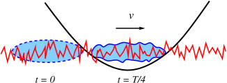
Figure 1: (Color online) Sketch of the experimental scenario in question. The zigzag line corresponds to the speckle potential that is superimposed onto the smooth harmonic potential. The condensate (shown in blue) is shifted to one edge of the trap and released at $t=0$, resulting in dipole oscillations.

Among other types of collective oscillations exhibited by the trapped condensates, of special significance is the dipole mode. It corresponds to the center of mass motion of the condensate which due to the harmonic confinement has the same frequency as the trap and is unaltered by interactions. In general, for 3D confinement, there exists a whole set of low energy modes that can be obtained analytically by solving the coupled hydrodynamic equations (derived from the GP equation above) for the velocity, ${\bf v}({\bf r},t)$, and the density, $n({\bf r},t)$: $\partial n/\partial t+{\rm div}({\bf v}n)=0$ and $m\partial{\bf v}/\partial t+\nabla\left\{m{\bf v}^{2}/2+V_{{\rm ext}}+\lambda n\right\}=0$. These equations allow for solutions, where the condensate is oscillating as a whole stringari , with frequencies given by $\omega_{e}=\omega_{{\rm ho}}\sqrt{2n_{r}^{2}+2n_{r}\ell+3n_{r}+\ell}$, assuming $V_{{\rm ext}}({\bf r})$ is harmonic with frequency $\omega_{{\rm ho}}$. The dipole mode is the one with quantum numbers $(n_{r}=0,\ell=1)$. In the absence of any other potential (disordered or not), the harmonic trap is special, leaving the center-of-mass motion completely decoupled from the relative degrees of freedom even for large amplitudes. However this feature is immediately lost as soon as any other external potential, e.g. disorder, is turned on, resulting in coupling of different modes, eventually leading to the complete decay of a well defined oscillating mode.

III Key Concepts

Our model consists of two main ingredients, disorder and inhomogeneity, which we describe below.

III.1 Disorder

For treating disorder within an analytic approach, among several well established techniques in the literature replica ; methods , we find it convenient to use the replica method. The disorder potential $U_{{\rm d}}({\bf x})$ is described in terms of a Gaussian distribution function with a strength $\gamma$ such that $P[U_{{\rm d}}]=\exp[-1/(2\gamma^{2})\int{\rm d}{\bf x}{\rm d}{\bf x}^{\prime}U_{{\rm d}}({\bf x})K^{-1}({\bf x}-{\bf x}^{\prime})U_{{\rm d}}({\bf x}^{\prime})]$ and $K$ describes the spatial correlations replica . Such procedure automatically allows for a freedom in choosing the actual disorder potential, the details of which are quickly erased by multiple scattering. To further simplify our investigation, we consider a white noise correlation function $K({\bf x})\sim\delta({\bf x})$. Thus, $\langle U_{{\rm d}}({\bf x})\rangle_{{\rm dis}}=0$ and $\langle U_{{\rm d}}({\bf x})U_{{\rm d}}({\bf x}^{\prime})\rangle_{{\rm dis}}=\gamma^{2}\delta({\bf x}-{\bf x}^{\prime})$, where $\langle\cdot\cdot\cdot\rangle_{{\rm dis}}$ means averaging over disorder. However, the trick of using the replica method lies in following a particular procedure for taking the sequence of averages (quantum followed by disorder), essential for calculating observables. While the replica trick has been typically used in relation to Anderson localization of non-interacting electrons, we adopt it in the context of ultra-cold interacting atoms. A brief outline of this technique is provided in the Appendix. Aside from technical aspects, the replica trick allows for a systematic diagrammatic perturbation expansion within which all transport properties can be calculated, at least in principle.

III.2 Inhomogeneity

Next we use local density approximation (LDA) stringari to account for the inhomogeneous density distribution of the trapped condensate. This is achieved by defining a position dependent chemical potential,

$$\mu\rightarrow\mu({\bf r}) = \mu-V_{{\rm trap}}({\bf r}),$$ (1)

clearly justified in the Thomas-Fermi limit stringari , which is typically always the case for trapped-atom BEC experiments. Thus, the density of the stationary condensate in the absence of disorder is given by

$$\rho({\bf r})=\mu({\bf r})/\lambda$$ (2)

Further, we assume that as the condensate undergoes dipole oscillations, on average the shape of the condensate is retained, meaning $\rho({\bf r}+{\bf r_{\rm cm}}(t))=\rho({\bf r})$. This is an extremely good assumption, it stems from the rigidity associated with the Bose condensate. This greatly simplifies the problem by allowing us to define all the relevant quantities locally, for example we define the local Bogoliubov excitation energies ripka

$$\Lambda_{{\bf k}}[{\bf r}]=\sqrt{e_{k}^{2}-\lambda^{2}\rho({\bf r})^{2}}$$ (3)

with $e_{k}=\hbar^{2}k^{2}/2m+\lambda\rho({\bf r})$. Also, from the linear part of the above dispersion relation, we can define a local sound velocity

$$c[{\bf r}]=\sqrt{\lambda\rho({\bf r})/m}.$$

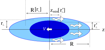
Figure 2: (Color online) Sketch showing the different relevant distances defined in the text. Dark (light) blue color represent spatial regions of the condensate where the local sound velocity is greater (lesser) than the center-of-mass velocity. Graphic arrows indicate excitation moving along the $z$ direction.

IV The Model

The total Hamiltonian for the problem can be written as the sum

$$\hat{H} = \underbrace{\hat{H}_{{\rm free}}+\hat{H}_{{\rm int}}}+\hat{V}_{{\rm trap}}+\hat{U}_{{\rm d}}$$

$$= \hskip 21.05519pt\underbrace{\hat{H}_{{\rm eff}}\hskip 12.80365pt+\hat{V}_{{\rm trap}}}+\underbrace{\hat{U}_{{\rm d}}}$$

$$\hskip 39.83368pt{\rm LDA}\hskip 28.45274pt{\rm replica},$$

where $\hat{H}_{{\rm free}}$ is for the free non-interacting atoms and $\hat{H}_{{\rm int}}$ is due to the atom-atom interaction. As indicated above, we first write an effective Hamiltonian for the bosons in the absence of any potentials by treating $\hat{H}_{{\rm int}}$ at the mean field level. Diagonalizing $\hat{H}_{{\rm eff}}$, the lowest eigenvalue corresponds to the condensate mode at temperatures $T<T_{{\rm BEC}}$. The excitations above the ground state are nothing but the Bogoliubov modes described above and are orthogonal to the condensate mode. Any other external potential will in general couple these different eigenmodes. However, as mentioned earlier, the trapping potential is typically smooth and LDA holds, drastically simplifying the calculation. The only piece that remains to be included is the potential, $\hat{U}_{{\rm d}}$. At any spatial location, the disorder tends to deplete the condensate by populating the Bogoliubov modes. However, this does not happen if the condensate is at rest, with zero center-of-mass velocity. Due to the superfluid property of the BEC, Landau criterion holds and there is a non-zero critical velocity below which no excitations can be generated and the nonequilibrium state will persist forever. This is precisely where the finite size of the condensate plays an important role. At any given center-of-mass velocity $v$, on the contrary, there is always a finite region of the condensate, shown by the light blue color in Fig. 2, where $v>c[{\bf r}]$ thus satisfying Landau criterion for excitations and providing a channel for the energy to be transferred from the center-of-mass motion to the Bogoliubov modes. In essence, this is the physical mechanism that provides the frictional force responsible for slowing down the condensate center-of-mass motion.
Remark: Before we proceed to calculations, we need to take into account the fact that, previously, excitations were calculated in the rest frame of the condensate. Thus, if we wish to continue calculating everything else in the same frame, it implies having to use a time dependent disorder potential.
This is certainly a non-trivial complication and cannot be simply neglected. Fortunately, LDA turns out to be perfectly suited for such a situation. It allows us to work in the lab frame instead, hence static disorder. Now, from Eq. (3), the locally defined Bogoliubov modes are eigenstates of momentum and hence remain unaltered under a Galilean frame transformation, only their energies are shifted according to:

$$\Lambda_{\bf k}\rightarrow\Lambda_{\bf k}^{{\rm lab}} = \Lambda_{\bf k}-\hbar{\bf k}\cdot{\bf v}.$$

Thus, we have gathered all the ingredients for conducting the transport calculations via the diagrammatics of the replica trick. The above model is quite general and allows for calculating observables in a broad range of scenarios by including appropriate orders in the perturbation expansion. For example, if the time scale of interest is larger than the Heisenberg time (time scale defined by the trapping potential), one needs to include appropriate particle-hole diagrams to describe the diffusive dynamics. On the other hand, if the dynamics occurs on the trap scale, then depending on the disorder strength, appropriate single particle diagrams may be sufficient. The only point one needs to remember is that the bare propagators of the replica theory are those for the quasiparticles representing atoms dressed by interactions with the corresponding Green’s function given by ripka ; mahan :

$$\mathscr{G}({\bf k},i\omega_{n})[{\bf r}]=\frac{1}{\Lambda_{{\bf k}}^{{\rm lab}}[{\bf r}]-i\omega_{n}}+\frac{1}{\Lambda_{{\bf k}}^{{\rm lab}}[{\bf r}]+i\omega_{n}},$$

where $\omega_{n}$ is the bosonic Matsubara frequency.

V Experiment

As elaborated in the introduction, our model is motivated by recent experiments performed on cold trapped atomic condensates. Hence, we illustrate the applicability of the model by considering the actual experimental situation of Refs. randy ; randy2 : ${}^{7}{\rm Li}$ atoms trapped in an axial harmonic trap with $\omega_{z}=2\pi\times 5.5\,\,{\rm Hz}$, aspect ratio $\alpha=\omega_{\perp}/\omega_{z}\approx 46$. The $s$-wave scattering length is tuned via a Feshbach resonance to about $a=25\,a_{{\rm B}}$, resulting in an axial condensate with the size represented by the Thomas-Fermi (TF) radius, which in units of the axial oscillator length $\ell_{z}$, is given by $R\approx 13.6\,\ell_{z}$. These parameters conform with the experimental data for damping of the BEC dipole mode used in the plot of Fig. 3. The disorder potential is produced using an optical speckle with gaussian correlation:

$$\langle U_{{\rm d}}({\bf x})U_{{\rm d}}({\bf x}^{\prime})\rangle_{{\rm dis}} = V_{{\rm d}}^{2}\exp\left[-\frac{2({\bf x}-{\bf x}^{\prime})^{2}}{\sigma^{2}}\right].$$ (4)

Further, while no data on temperature is available, from the observations presented, it is safe to assume that the experiment is conducted at temperatures well below $T_{{\rm BEC}}$ and thus a $T=0$ theoretical prescription should suffice.

The TF density of the stationary condensate in cylindrical coordinates follows from Eqs. (1) and (2)

$$\rho(r_{\perp},z) = \frac{m\omega_{z}^{2}(R^{2}-\alpha^{2}r_{\perp}^{2}-z^{2})}{2\lambda},$$

with the normalization fixed by the TF axial size $R$ via

$$N=4\pi\int_{0}^{R/\alpha}\int_{0}^{R[r_{\perp}]}\rho(r_{\perp},z){\rm d}z\,\,r_{\perp}{\rm d}r_{\perp},$$ (5)

with the different distances indicated in Fig. 2. For convenience, we define the dimensionless ratio $\xi[r_{\perp}]=v/c[r_{\perp}]$, where $c[r_{\perp}]$ is the speed of sound at the coordinate $\{r_{\perp},z=0\}$. We also use the notation, $c\equiv c[0]$ and $\xi\equiv\xi[0]$. We point out that even though the aspect ratio is large, the chemical potential $\mu\sim{\cal O}(\hbar\omega_{\perp})$, hence a full 3D treatment is required. Finally, we observe that the oscillation data shown in Fig. 3 indicates dynamics over time scales much shorter than the diffusion time dictated by the disorder. This greatly reduces the manipulations and it suffices to calculate only the single particle diagrams. The imaginary part of the selfenergy, obtained from the dressed propagator of the non-interacting quasiparticles, immediately provides the transition rate $W({\bf k}\rightarrow{\bf k}^{\prime},{\bf r})$ at the spatial point ${\bf r}$ (for details refer to the Appendix). However, we alert the reader that one typically never measures the single particle propagator in an experiment and we still need to connect to the damping of the classical dipole mode. We achieve this by recalling that the energy per condensate particle is nothing but the chemical potential $\mu({\bf r})$. Thus, the total energy transfer rate out of the ${\bf k=0}$ condensate mode is precisely

$$\Gamma=\int_{\Omega}{\rm d}{\bf r}\int_{k>\kappa}{\rm d}{\bf k}\,\,\mu({\bf r})W(0\rightarrow{\bf k},{\bf r}),$$ (6)

where $\kappa$ is some infrared cutoff imposed by the trapping potential and $\Omega$ is the condensate volume. The above integral can be approximated and has a nice analytic form if excitations are allowed only along the axial (z) direction. This constraint can be understood to arise from the high aspect ratio $\alpha$ of the trapping potential. Even at large $k$, where this approximation may fail, we expect the density of states to be diminished enough to accrue any appreciable error. With this we arrive at the final result in terms of dimensionless quantities represented by $(\bar{\,\,\,\,})$(physical quantities scaled in units of the axial harmonic trap: lengths in units of $\ell_{z}=\sqrt{\hbar/m\omega_{z}}$ and energies in $\hbar\omega_{z}$)

$$\bar{\Gamma}[\xi]=\frac{\bar{\gamma}^{2}\bar{R}^{4}}{4\sqrt{2}\pi\bar{a}}\int_{0}^{1}t^{2}\,\,{\cal I}[\xi/\sqrt{t},\xi_{{\rm min}}/\sqrt{t}]\,\,{\rm d}t,$$ (7)

where the upper (lower) integration limit corresponds to the center (radial edge) of the condensate, $\xi_{{\rm min}}$ is related to $\kappa$, $\xi_{{\rm min}}=\hbar\kappa/2mc$ and the function ${\cal I}$ is defined by Eqs. (13) and (14) of Appendix.

VI Results and Discussion

To begin with, we first look at the plot in Fig. 3(a) that shows the velocity dependence of the function ${\cal I}$ for points along the long axis of the condensate. The sharp discontinuity near the speed of sound $c$ is a clear indication of the origin of distinct regimes of damping as the BEC flows through the disordered medium. Essentially, for velocities significantly smaller than the speed of sound $c$, excitations are only allowed in a small shell near the surface of the condensate. This region tends to grow inwards, eventually allowing excitations everywhere in the condensate, as the center-of-mass velocity reaches $c$. However, increasing the velocity beyond this critical value, the excited volume remains fixed while the Bogoliubov density of states keeps falling, resulting in net decay of the damping rate with velocity.

The above expression for $\bar{\Gamma}$ represents the first of the two main results of this article. It conveniently leads us to a dynamical equation for the condensate motion, if we picture the BEC oscillating in the random potential as a rigid body whose hydrodynamic oscillations are damped as the kinetic energy is transferred to the internal excitations. Such damped oscillatory motion of the BEC center-of-mass coordinate can easily be described by an equation for the peak velocity of the condensate motion in terms of $\xi_{{\rm peak}}$

$$\frac{\partial\xi_{{\rm peak}}}{\partial t}=-\frac{2}{N\bar{R}^{2}\xi_{{\rm peak}}}\tilde{\Gamma}[\xi_{{\rm peak}}]=-\beta\xi_{{\rm peak}},$$ (8)

where the energy dissipation rate is averaged over one oscillation period, represented by $\tilde{\Gamma}=(1/T)\int_{0}^{T}\Gamma{\rm d}t$. The above equation for $\xi_{{\rm peak}}$ represents the second main result of this article. These results immediately provide important asymptotic exponents governing the dependence of the velocity-damping rate $\beta$ on the scattering length. For this, all that is required is to remember that the total number of atoms $N$ is fixed, automatically implying $R\sim a^{1/5}$ from the normalization condition Eq.  (5); thus, $c\sim a^{1/5}$ follows as well. Now, from the functional form given by Eq. (14),

$$\beta\sim\left\{\begin{array}[]{l}a^{-6/5}\,\,\,\,\forall\,\,\xi\ll 1\Rightarrow{\cal I}\sim 1/a\\ a^{0}\,\,\,\,\,\,\,\,\,\,\,\,\,\forall\,\,\xi\gg 1\end{array}\right.$$ (11)

The latter limit is easily confirmed from the plot, Fig. 10, in Ref. randy2 . While, data for the former limit is not present in the same figure, available data points for $\xi<1$ show a clear trend towards the predicted limiting behavior. Instead, we indirectly verify this limit by extracting the damping rate as a function of $\xi$ from the data shown in Fig. 3(b) which can then be written as a function of scattering length, $a$, by fixing $v$ in Eq. (7). We again find very good agreement, confirming the exponent corresponding to the former limit as well.

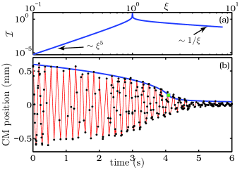
Figure 3: (Color online) (a) Damping function along the long axis of the condensate plotted as a function of $\xi$. (b) Thick solid curve: theoretical prediction for the peak center-of-mass displacement of the condensate as a function of time for $\bar{\gamma}=0.5$, filled circles connected with thin line are experimental data points for the center-of-mass position as the condensate oscillates in the trap randy2 . Square marker indicates the point where $\xi_{{\rm peak}}=1$.

The only parameter that remains to be estimated is the $\delta$-correlated disorder strength $\gamma$. We remind the reader that, in the actual experiment, the disorder potential, Eq.  (4), has a finite correlation length $\sigma$. Such spatial correlations are indeed outside the scope of the current LDA based model. Therefore, $\gamma$ in our model maybe considered as a free parameter representing the renormalized value of the disorder strength. Our result, the solution of Eq. (8) plotted in Fig. 3(b), is in excellent quantitative agreement with the experimental data, indicating the validity of a delta-correlated ansatz for the speckle potential. The proposed model is also able to capture all the damping time scales via only coupling to the Bogoliubov excitations. Thus, we identify the most dominant source of dissipation, sufficient to describe transport in such ultra-cold trapped-atom experiments.

Finally, we shall comment on the strength of the disorder. For this, let us use the value of $\bar{\gamma}$ estimated in Fig. 3(b) to find the magnitude of disorder-induced condensate depletion given via the method of Ref. huang

$$\rho_{{\rm dep}}(0) = \frac{m^{2}\gamma^{2}}{8\pi^{3/2}\hbar^{4}}\sqrt{\frac{\rho(0)}{a}}.$$

We find $\rho_{{\rm dep}}(0)/\rho(0)=.002$, implying that the condensate density remains almost unchanged after inclusion of speckle potential and thus justifying the assumption of weak disorder, permitting perturbative treatment up to second order in disorder strength. Furthermore, it also points to an important aspect about the disorder potential used in the experiment randy2 . There, even though the disorder strength seems to be large, given by $V_{{\rm d}}\approx 0.6\,\mu$, our theoretical model points to a critical interplay between disorder correlations and interactions, resulting in a dressed disorder with a small renormalized strength $\gamma$.

VII Conclusion

To summarize, we have given a theory for describing the transport properties of finite-size atomic condensates flowing through disorder potentials. We emphasize the intricate role played by the inhomogeneous character of the condensate, resulting in a completely different form of the damping function, ${\cal I}$, above and below the critical velocity, $c$. The validity of our model is established via comparison with the experimental observations of damped hydrodynamic dipole oscillations of the condensate randy2 . The predicted power-law dependance of the damping on the interaction parameter is in excellent agreement with experimental observations. Our results, while based on a white noise disorder model, show extremely good agreement with experimental data, thereby, indicating the insignificant role of finite correlations in determining the dissipation time scales. While a full theory was not necessary for the aspects considered here, an improved quantitative picture can be realized by including finite disorder-correlations, for example, via a coherent potential approximation cpadig . Such procedure leads to an effective, renormalized disorder vertex, whose value can then be compared with the $\gamma$ obtained here. However, these calculations are beyond the current model and would be considered in a future work. Furthermore, although the effects of Anderson localization turn out not to be relevant for these experimentsrandy ; randy2 , we predict they could be if the center-of-mass motion is very slow and therefore the physics is dominated by diffusion. These effects could be incorporated into our calculations by including appropriate diagrams corresponding to particle-hole processes. Finally, the analysis presented here can be easily translated in the language of friction indicating the manifestation of non-linear friction on mesoscopic quantum objects.

Appendix A Replica Method

The difficulty of disorder averaging is eliminated using the standard replica trick of considering $R$ replicas of the same field with the understanding that the $R\rightarrow 0$ limit is taken at the end. However, this procedure comes with a cost, it leads to an effective attractive interaction between atoms from different replicas. To illustrate this, we simply write down the full average of some operator $\hat{{\cal O}}$, as

$$\langle\hat{{\cal O}}\rangle = \lim_{R\rightarrow 0}\left[\frac{1}{R}\frac{\partial\langle{\cal Z}^{R}[\eta]\rangle_{{\rm dis}}}{\partial\eta}\right],$$ (12)

where $\eta$ is some source field, and ${\cal Z}^{R}[\eta]$ is the partition function of the replicated boson field $\{(\psi^{a\dagger},\psi^{a}),a=1,..,R\}$. Thus, essentially it involves an averaging of the partition function over the distribution, $P[U_{{\rm d}}]$, that can be carried out quite easily using Gaussian integration resulting in an effective action

$$S_{{\rm eff}} = \sum_{a=1}^{R}S_{{\rm clean}}[\psi^{a},\psi^{a\dagger}]+\sum_{a,b=1}^{R}S_{{\rm replica}}[\psi^{a},\psi^{b},\psi^{a\dagger},\psi^{b\dagger}],$$

with

$$S_{{\rm replica}} = -\frac{\gamma^{2}}{2}\sum_{m,n}\int{\rm d}{\bf x}~{}\psi_{m}^{a\dagger}({\bf x})\psi_{m}^{a}({\bf x})\psi_{n}^{b\dagger}({\bf x})\psi_{n}^{b}({\bf x}),$$

where $S_{{\rm clean}}$ is the action in the absence of disorder, and index $m$ and $n$ are introduced to indicate Matsubara frequencies $\omega_{m}$ and $\omega_{n}$, respectively. Thus, the additional replica-induced action represents interactions between atoms of different replica index with the disorder vertex represented by the Feynman diagram of Fig. 4(a). Also, it does not involve energy exchange between replicas since the disorder potential is intrinsically time independent.

Appendix B Damping Function

The relevant diagrams are the single particle ones as shown in Fig. 4(b)-(e). A technical point of interest is that the contribution of diagrams containing loops of the type shown in Fig. 4(b) tend to zero due to the limit $R\rightarrow 0$ in Eq. (12). In essence, the replica trick eliminates all diagrams that are disconnected before the disorder averaging, thus vastly reducing the computation.

For the particular experimental situation considered here, it suffices to include just the leading order diagrams. Further, the $T=0$ nature of the experiment makes the use of replica trick redundant and the result coincides with the Fermi’s golden rule. However, we remind the reader that the model itself is more general and maybe applied to other situations as mentioned in the text. All throughout, our goal has been to provide a theoretical model to describe transport in trapped, disordered, ultra-cold atomic experiments in general.

Figure 4: Diagram contributions to the self energy: (a) corresponds to the disorder vertex, $m$ and $n$ are replica index. (b) and (c) are second order, (c) and (d) are fourth order contributions to the selfenergy. The external lines are not to be included for selfenergy calculations. The solid lines represent the quasiparticle propagator.

Thus, the formal expression for the transition rate is given simply by the imaginary part of selfenergy (diagram of Fig. 4(c)).

$$W(0\rightarrow{\bf k},{\bf r})=\frac{2\pi\gamma^{2}}{\hbar}\rho({\bf r})(u_{\bf k}[{\bf r}]-v_{\bf k}[{\bf r}])^{2}\delta(\Lambda_{\bf k}[{\bf r}]-\hbar{\bf k}\cdot{\bf v}),$$

where $u_{{\bf k}}$ and $v_{{\bf k}}$ are the amplitudes that define Bogoliubov quasiparticles and are related to the energy $\Lambda_{{\bf k}}=\sqrt{e_{k}^{2}-\lambda^{2}\rho^{2}}$ by $u_{{\bf k}}^{2}=(e_{k}/\Lambda_{k}+1)/2$ and $v_{{\bf k}}^{2}=(e_{k}/\Lambda_{k}-1)/2$ with $e_{k}=\hbar^{2}k^{2}/2m+\lambda\rho$. Therefore, the full expression for the loss rate $\Gamma$ can be written simply by substituting in Eq. (6) of text. Performing the $z$ and the $k$ integration we arrive at

$$\Gamma = \frac{2\pi\gamma^{2}m^{2}\omega_{z}^{3}}{\pi\sqrt{2}\hbar^{2}\lambda R_{\perp}^{2}}\int_{0}^{R/\alpha}r_{\perp}{\rm d}r_{\perp}R[r_{\perp}]^{4}{\cal I}[\xi[r_{\perp}],\xi_{{\rm min}}[r_{\perp}]],$$

where $R[r_{\perp}]$, indicated in Fig. 2, is written as $R[r_{\perp}]=\sqrt{R^{2}-\alpha^{2}r_{\perp}^{2}}$ and the function ${\cal I}$ is defined in terms of the boundary function ${\cal F}$

$${\cal I}[p,q]=\left\{\begin{array}[]{lr}{\cal F}(1,p)-{\cal F}(0,p),&\forall p\geq\sqrt{1+q^{2}}\\ {\cal F}(1,p)-{\cal F}(\sqrt{1-p^{2}+q^{2}},p),&\forall p<\sqrt{1+q^{2}}\end{array},\right.$$ (13)

with

$${\cal F}(y,x) = \frac{1}{8}\left[y(-5+2y^{2}-3x^{2})\sqrt{-1+x^{2}+y^{2}}+\right.$$ (14)

$$\left.(3+2x^{2}+3x^{4})\log\left(2y+2\sqrt{-1+y^{2}+x^{2}}\right)\right].$$

Now, with straightforward manipulation, one can immediately show that Eq. (7) of text follows by simply expressing all quantities in dimensionless units.

References

- (1) S. G. Bhongale and Eddy Timmermans, Phys. Rev. Lett. 100, 185301 (2008); J. M. Obrecht, R. J. Wild, M. Antezza, L. P. Pitaevskii, S. Stringari, and E. A. Cornell, Phys. Rev. Lett. 98, 063201 (2007); M. Vengalattore, J. M. Higbie, S. R. Leslie, J. Guzman, L. E. Sadler, and D. M. Stamper-Kurn, Phys. Rev. Lett. 98, 200801 (2007); S. Stringari, Phys. Rev. Lett. 86, 4725 (2001).
- (2) P. Krüger, et al. J. Phys. Conf. Series 19, 56 (2005).
- (3) M. H. W. Chan, K. I. Blum, S. Q. Murphy, G. K. S. Wong, and J. D. Reppy, Phys. Rev. Lett. 61, 1950 (1988); G. K. S. Wong, P. A. Crowell, H. A. Cho, and J. D. Reppy, Phys. Rev. Lett. 65, 2410 (1990).
- (4) K. Huang and H. -F. Meng, Phys. Rev. Lett. 69, 644 (1992).
- (5) S. Giorgini, L. Pitaevskii, and S. Stringari, Phys. Rev. B 49, 12938 (1994).
- (6) Y. P. Chen et al., Phys. Rev. A 77, 033632 (2008).
- (7) D. Dries, S. E. Pollack, J. M. Hitchcock, and R. G. Hulet, Phys. Rev. A 82, 033603 (2010).
- (8) M. Pasienski, D. McKay, M. White, and B. DeMarco, arXiv:0908.1182.
- (9) P. Nozieres and D. Pines in The Theory of Quantum Liquids (Perseus Books, Cambridge, MA, 1999).
- (10) M. Urbakh, J. Klafter, D. Gourdon, and J. Israelachvili, Nature 430, 525 (2004).
- (11) G. Raoti et al., Nature 453, 895 (2008).
- (12) J. Billy et al., Nature 453, 891 (2008).
- (13) P. W. Anderson, Phys. Rev. 109, 1492 (1958).
- (14) C. Chin et al., Science 305, 1128 (2004); C. A. Regal, M. Greiner, and D. S. Jin, Phys. Rev. Lett. 92, 040403 (2004); T. Bourdel et al., Phys. Rev. Lett. 93, 050401 (2004); K. M. O’Hara, S. L. Hemmer, M. E. Gehm, S. R. Granade, and J. E. Thomas, Science 298, 2179 (2002).
- (15) M. Albert, T. Paul, N. Pavloff, and P. Leboeuf, Phys. Rev. Lett. 100, 250405 (2008).
- (16) S. E. Skipetrov and B. A. van Tiggelen, Phys. Rev. Lett. 92, 113901 (2004).
- (17) L. Pitaevskii and S. Stringari, in Bose-Einstein Condensation (Oxford University Press, UK, 2004).
- (18) S. F. Edwards and P. W. Anderson, J. Phys. F 5, 965 (1975).
- (19) For supersymmetry method see K. B. Efetov, Sov. Phys. JETP 55, 514 (1982); For Keldysh method see A. Kamenev, cond-mat/0412296.
- (20) J. -P. Blaizot and G. Ripka, in Quantum Theory of Finite Systems (MIT Press, Cambridge MA, 1985).
- (21) G. D. Mahan, in Many-particle physics, 2nd ed. (Plenum Press, NY, 1990).
- (22) E. J. S. Lage and R. B. Stinchcombe, J. Phys. C 10, 295 (1977).