Exact time-reversal focusing of acoustic and quantum excitations in open cavities: The perfect inverse filter

Abstract

The time-reversal mirror (TRM) prescribes the reverse playback of a signal to focalize an acoustic excitation as a Loschmidt echo. In the quantum domain, the perfect inverse filter (PIF) processes this signal to ensure an exact reversion provided that the excitation originated outside the cavity delimited by the transducers. We show that PIF takes a simple form when the initial excitation is created inside this cavity. This also applies to the acoustical case, where it corrects the TRM and improves the design of an acoustic bazooka. We solve an open chaotic cavity modeling a quantum bazooka and a simple model for a Helmholtz resonator, showing that the PIF becomes decisive to compensate the group velocities involved in a highly localized excitation and to achieve subwavelength resolution.

I Introduction

The time-reversal mirror (TRM) technique was developed by Mathias Fink and collab. FinkSA in order to refocus an ultrasonic excitation diffusing away through a heterogeneous medium. The remarkable robustness of this technique against inhomogeneities and imperfections in the procedure enabled novel applications in medical physics Montaldo , oceanography Edelman and telecommunications Henty . The acoustic signals emerging from a localized source point are recorded by an array of transducers. Ideally, this array splits the system in two portions: the internal cavity, where the focusing takes place, and the outer region, towards where the excitation finally spreads away. The transducers then play-back each registry in the inverted time sequence. Surprisingly, this simple prescription allows recovering the initial excitation with high precision. This constitutes an alternative form of achieving a Loschmidt Echo Jalabert , i.e. the time reversal of an excitation distributed in a complex medium. To ensure the exact reversed dynamics, we exploited the close correspondence between the Schrödinger and the classical wave equations DeRosny ; CalvoPB by introducing a formal prescription denoted as the perfect inverse filter (PIF) PastawskiEPL . This yields the precise injection function that produces the targeted dynamics inside the cavity. In particular, the PIF prescribes how to process the recorded signal in order to achieve the exact refocusing of whatever excitation exists in the cavity, provided that it was originated as a wave packet incoming from the outer region. A potential application is the quantum bazooka, analogous to the acoustic bazooka conceived by M. Fink and collaborators Kuperman . When a waveguide injects a well-defined wave packet into a chaotic cavity, it is reflected as a persistent noisy signal. The time-reversed counterpart allows to store in the cavity the weak signal injected through a long period of time until it emerges as a burst of excitation.

To further optimize the spatial contrast of a localized acoustic excitation in cases where TRM results imperfect, Fink and collab. proposed the spatio-temporal inverse filter (STIF) Tanter . It requires the inversion of a matrix built from the Fourier transforms of the direct wavefield propagators. These give the response at the transducers to a Dirac delta signal in each control point within the focal region. Unlike the TRM, the STIF results in a highly invasive technique. Minimally invasive STIF (miSTIF), a recent proposal by Vignon et al. Vignon , achieves the same focusing quality as STIF without resorting to control points. All the information in the wavefield propagator is deduced from the backscattering signals of the transducers and the technique results no more invasive than TRM. Both the miSTIF and the PIF involve the inversion of a propagator matrix in the reduced basis of the transducers. However, this may result in numerical instabilities that require a delicate regularization procedure to deal with the Green’s function divergencies.

In this work, we assume a natural separation between the incoming and outgoing excitation components, as when the source is internal, to develop a PIF procedure based on the detection of the escaping wave. This internal PIF results very simple and intrinsically stable. Moreover, it reveals a property not obvious before: the filter that corrects the TRM does not depend on the internal scattering, but only on the group velocities of the various propagating modes in the far field region. This is general enough to cover, either exactly or as an approximation, a wide range of TRM set-ups that would benefit from a PIF. We may mention subwavelength focusing FinkSCIENCE , lithotripsy in dispersive media Montaldo , the quantification of nonlinear media Ulrich , coherent control of optical excitation energies in nanoplasmonic systems Stockman and acoustic bazookas Kuperman . To this list we may add the development of novel coherent control strategies that seek the local injection of designed quantum excitations. As discussed below, this involves fields as diverse as nanoelectromechanics, Bose-Einstein condensates and NMR.

We start by considering a quantum system where the corresponding propagators are well known CalvoPRL . Then, we will show that the resulting PIF prescription remains valid to describe sound propagation. A numerical contrast with the TRM procedure in two situations of physical interest, the quantum bazooka configuration and a simplified model for a Helmholtz resonator coupled to a grated waveguide, confirms the relevance of the PIF correction.

II Time-reversal in a cavity

We consider the situation in which, at the initial time, the excitation is concentrated inside the cavity. From $t_{0}=0$ until a registration time $t_{R}$, the discrete wave function

$$\psi_{s}(t)=\sum\nolimits_{n}\mathrm{i}\hbar G_{s,n}^{R}(t)\psi_{n}(0),\text{ }0\leq t\leq t_{R},$$ (1)

is detected and recorded as it escapes through the frontier. In the present letter we consider a cavity, either integrable or chaotic, open through a 1d channel. Therefore, its frontier is controlled by a single transducer at $x_{s}=sa$, with $s$ integer and $a$ the distance between neighbors sites in a lattice. Although apparently a restriction, this simple model faithfully represents the essential underlying physics. A straightforward generalization requires a matrix formulation and will be presented elsewhere.

Here, $G_{m,n}^{R}(t)$ is the retarded Green’s function relating the amplitude response at $x_{m}$ when a Dirac delta signal $\delta(t)$ is injected at $x_{n}$ inside the cavity. It satisfies the inhomogeneous Schrödinger equation

$$\mathrm{i}\hbar\frac{\partial}{\partial t}G_{m,n}^{R}(t)-\sum\nolimits_{i}H_{m,i}G_{i,n}^{R}(t)=\delta_{m,n}\delta(t),$$ (2)

with $H_{m,i}$ the Hamiltonian matrix elements. Assuming that there are no localized states, the registration time $t_{R}$ is taken long enough in order to ensure that all excitations have left the cavity.

As we have shown in ref.PastawskiEPL , the time reversion for a wave packet arriving at the cavity from the outer region is performed, in the energy domain, through the injection

$$\chi_{s}(\varepsilon)=\frac{1}{\mathrm{i}\hbar G_{s,s}^{R}(\varepsilon)}\psi_{s}^{\mathrm{rev}}(\varepsilon).$$ (3)

Notice that in the above expression,

$$\psi_{s}^{\mathrm{rev}}(\varepsilon)\equiv\int_{-\infty}^{\infty}\mathrm{d}te^{\mathrm{i}\varepsilon t/\hbar}\psi_{s}^{\mathrm{rev}}(t),$$ (4)

accounts for the time reversed complete evolution of the wave packet, i.e. both the incoming and outgoing components are required in order to compute $\psi_{s}^{\mathrm{rev}}(t)$. In the present work we want to reverse the signal that is produced inside the cavity. Then, we deal with the building up of the complete evolution from the knowledge of $\psi_{s}(t)$ at times $0\leq t\leq t_{R}$. On the assumption that the injection function is known, the reversed propagation at the transducer would be

$$\psi_{s}^{\mathrm{rev}}(t) =\psi_{s}^{\ast}(2t_{R}-t)$$ (5)

$$=\mathrm{i}\hbar\int_{0}^{t}G_{s,s}^{R}(t-t^{\prime})\chi(x_{s},t^{\prime})\mathrm{d}t^{\prime},$$ (6)

for times $t_{R}\leq t\leq 2t_{R}$ before the focalization. Since the PIF prescription achieves exact reversion inside the cavity, the evolution at subsequent times ($t>2t_{R}$) can be conceived as the wave packet that starts at the focalization time with $\psi_{n}(2t_{R})=\psi_{n}^{\ast}(0)$. Thus, for subsequent times we expect

$$\psi_{s}^{\mathrm{rev}}(t)=\sum\limits_{n}\mathrm{i}\hbar G_{s,n}^{R}(t-2t_{R})\psi_{n}^{\ast}(0).$$ (7)

A comparison between eqs.(1) and (7) shows that for the most simple case in which all coefficients $\psi_{n}(0)$ are real, both evolutions become identical. The same evolution but sign changed should be obtained when they are purely imaginary. In a more general situation where the coefficients present different phases we start with the Fourier transform

$$\psi_{s}^{\mathrm{rev}}(\varepsilon) =\int_{t_{R}}^{2t_{R}}\psi_{s}^{\ast}(2t_{R}-t)e^{\mathrm{i}\varepsilon t/\hbar}\mathrm{d}t+$$ (8)

$$+\mathrm{i}\hbar\sum\limits_{n}\int_{2t_{R}}^{\infty}G_{s,n}^{R}(t-2t_{R})\psi_{n}^{\ast}(0)e^{\mathrm{i}\varepsilon t/\hbar}\mathrm{d}t$$ (9)

$$=e^{\mathrm{i}\varepsilon 2t_{R}/\hbar}\left[\psi_{s}^{\ast}(\varepsilon)+\mathrm{i}\hbar\sum\limits_{n}G_{s,n}^{R}(\varepsilon)\psi_{n}^{\ast}(0)\right],$$ (10)

where the second term within the brackets can be interpreted as the unknown evolution for subsequent times. The $\varepsilon$ argument and the superscript in $G_{s,n}^{R}(\varepsilon)$ are omitted for a compact notation henceforth. At this point, we account for the hopping terms $V_{s,s-1}$ and $V_{s-1,s}$ (with $x_{s-1}$ inside de cavity) connecting the cavity with the outer region. Hence, we use the Dyson equation Economou to rewrite

$$G_{s,n}=G_{s,n}^{(0)}+G_{s,s}V_{s,s-1}G_{s-1,n}^{(0)},$$ (11)

where $G^{(0)}$ follows eq.(2) for the unperturbed Hamiltonian with $V_{s,s-1}=V_{s-1,s}=0$. Since $s$ and $n$ are at disconnected subsystems $G_{s,n}^{(0)}=0$. Besides, since the cavity subsystem is closed and non absorbing, $V_{s,s-1}G_{s-1,n}^{(0)}$ is a real number. Therefore, we obtain for the unknown evolution

$$\mathrm{i}\hbar\sum\limits_{n}G_{s,n}\psi_{n}^{\ast}(0)=-\frac{G_{s,s}}{G_{s,s}^{\ast}}\psi_{s}^{\ast}(\varepsilon).$$ (12a)

Finally, we use this last expression to rewrite eq.(10) as

$$\psi_{s}^{\mathrm{rev}}(\varepsilon)=e^{\mathrm{i}\varepsilon 2t_{R}/\hbar}\left[1-\frac{G_{s,s}}{G_{s,s}^{\ast}}\right]\psi_{s}^{\ast}(\varepsilon).$$ (13)

Since we have the complete $\psi_{s}^{\mathrm{rev}}(\varepsilon)$, the injection function according to the PIF formula is given by

$$\chi_{s}(\varepsilon) =\frac{1}{\mathrm{i}\hbar G_{s,s}^{R}}\psi_{s}^{\mathrm{rev}}(\varepsilon)$$ (14)

$$=\frac{2}{\hbar}e^{\mathrm{i}\varepsilon 2t_{R}/\hbar}\mathrm{Im}\left(G_{s,s}^{-1}\right)\psi_{s}^{\ast}(\varepsilon).$$ (15)

This is the PIF prescription for the case where the initial state is an excitation inside the cavity. As we shall see, the imaginary component of the inverse in $G_{s,s}$ is closely related with the group velocity of the scattered waves in the outer region. Therefore, contrary to the external source condition presented in ref. PastawskiEPL , the correction imposed by the PIF in internal source condition does not depend on the structure of the cavity.

In this Letter, we used the one-dimensional picture for simplicity. Following the same reasoning as before, a multichannel generalization for the PIF procedure implies minor details and will be described elsewhere. In such case, one should be able to compute the relevant Green’s function components linking the transducers in the boundary through a matrix continued fraction algorithm PastawskiPRB . An alternative, more general formulation for the PIF may be obtained based on the fundamental optical theorem FoaTorres . In words, it states that the continuous density of states at a given site $x_{0}$ is built upon the escape rates through the boundaries of the system. If we choose a semi-infinite chain and there is no escape to the left of site $x_{0}$, the excitation can only escape to the right of the frontier $x_{s}$ with a rate $\mathrm{Im}\Sigma_{s}/\hbar$. In equations:

$$\mathrm{Im}G_{0,0}=G_{0,s}\mathrm{Im}\Sigma_{s}G_{s,0}^{\ast}.$$ (16)

Multiplying both sides by a pulse $\xi(\varepsilon)$ and the $\mathrm{i}\hbar$ factor we find

$$\mathrm{i}\hbar\left(G_{0,0}-G_{0,0}^{\ast}\right)\xi(\varepsilon)=2\mathrm{i}G_{0,s}\Gamma_{s}(-\mathrm{i}\hbar)G_{s,0}^{\ast}\xi(\varepsilon),$$ (17)

with $\Gamma_{s}=-\mathrm{Im}\Sigma_{s}$. Since the outgoing wave originated at the focal point writes

$$\psi_{0}(\varepsilon)=\mathrm{i}\hbar G_{0,0}\xi(\varepsilon),$$ (18)

we re-obtain the PIF formula by identifying the second term in the left hand of eq.(17) as the incoming wave that produced the pulse in the focal point. The complete evolution, identical to the reversed one, results

$$\psi_{0}(\varepsilon)+\psi_{0}^{\ast}(\varepsilon) =\psi_{0}^{\mathrm{rev}}(\varepsilon)$$ (19)

$$=\mathrm{i}\hbar G_{0,s}\left[\frac{2}{\hbar}\Gamma_{s}\psi_{s}^{\ast}(\varepsilon)\right].$$ (20)

The term between the square brackets is the excitation that must be injected at $x_{s}$ to reproduce the original signal in the cavity and coincides with the PIF prescription obtained in eq.(15).

II.1 PIF in a quantum bazooka configuration

In order to evaluate the eq.(15) we propose a model for a quantum bazooka device composed by a stadium billiard coupled with a one-dimensional waveguide as shown in the top of fig.(1). The discretization in the Schrödinger equation gives the tight-binding structure of the Hamiltonian

$$\hat{H}=\hat{H}_{B}+\hat{H}_{BC}+\sum_{j}\left(E_{j}\hat{c}_{j}^{{\dagger}}\hat{c}_{j}+V_{j,j+1}\hat{c}_{j+1}^{{\dagger}}\hat{c}_{j}+\mathrm{h.c.}\right),$$ (21)

where $\hat{H}_{B}$ is the Hamiltonian of the billard in a discrete basis and $\hat{H}_{BC}$ the coupling with the waveguide. In the waveguide, $E_{j}$ denotes the energy at site $x_{j}=ja$ and $V_{j,j+1}$ is the hopping amplitude between sites $x_{j}$ and $x_{j+1}$. Supposing a single semi-infinite waveguide, the cavity results delimited by a single transducer at site $x_{s}$. The Green’s function is obtained through the continued fraction technique as

$$G_{s,s}(\varepsilon)=\frac{1}{\varepsilon-E_{s}-\Sigma_{\mathrm{in}}(\varepsilon)-\Sigma_{\mathrm{out}}(\varepsilon)},$$ (22)

where $\Sigma_{\mathrm{in}}(\varepsilon)$ and $\Sigma_{\mathrm{out}}(\varepsilon)$ are the self-energy corrections due to the presence of sites inside and outside the cavity respectively Medina . Notice that the presence of the billard is included through $\Sigma_{\mathrm{in}}(\varepsilon)$.

Decimation on the cavity gives the $\Sigma_{\mathrm{in}}(\varepsilon)$ contribution as a continued fraction composed by the hoppings and the site energies. In absence of magnetic fields or dissipation those parameters are all real numbers. Therefore,

$$\Sigma_{\mathrm{in}}(\varepsilon)=\frac{V_{s,s-1}V_{s-1,s}}{\varepsilon-E_{s-1}-\dfrac{V_{s-1,s-2}V_{s-2,s-1}}{\varepsilon-E_{s-2}-\cdots\tfrac{V_{1,0}V_{0,1}}{\varepsilon-E_{0}-...}}},$$ (23)

is also a real function regardless the details of $H_{B}$.

On the other hand, in the limit where the number of sites increases indefinitely, the homogeneous outer region, a linear chain with site energies $E_{\mathrm{o}}$ and hoppings $V$, contributes to the self energy as a complex function Medina :

$$\Sigma_{\mathrm{out}}(\varepsilon)=\Delta(\varepsilon)-\mathrm{i}\Gamma(\varepsilon).$$ (24)

The relationship between $\Gamma(\varepsilon)$ and the group velocity can be found through the dispersion relation for the asymptotic waves:

$$\varepsilon_{k} =E_{\mathrm{o}}-2V\cos(ka),$$ (25)

$$v_{g} =\frac{1}{\hbar}\frac{\mathrm{d}\varepsilon_{k}}{\mathrm{d}k}=\frac{2Va}{\hbar}\sin(ka)=v_{\max}\sin(ka)$$ (26)

$$=\frac{2a}{\hbar}\sqrt{V^{2}-\left(\frac{\varepsilon_{k}-E_{\mathrm{o}}}{2}\right)^{2}}=\frac{2a}{\hbar}\Gamma(\varepsilon_{k}).$$ (27)

We choose $E_{\mathrm{o}}=2V$ so that the differential form of the Schrödinger equation for a particle with mass $m$ is obtained as the limit $\hbar^{2}/2Va^{2}\longrightarrow m$ when $V\rightarrow\infty$ and $a^{2}\rightarrow 0$. Since only the imaginary component from $\Sigma_{\mathrm{out}}(\varepsilon)$ is required, eq.(15) writes

$$\chi_{s}^{\mathrm{PIF}}(\varepsilon)=\frac{2}{\hbar}e^{\mathrm{i}\varepsilon 2t_{R}/\hbar}\Gamma(\varepsilon)\psi_{s}^{\ast}(\varepsilon).$$ (28)

The complex exponential serves to define the origin of time, and hence we can neglect it. Using the definition of $\Gamma(\varepsilon)$ given above we get

$$\chi_{s}^{\mathrm{PIF}}(\varepsilon) =\sqrt{1-\left(\frac{\varepsilon-2V}{2V}\right)^{2}}\tfrac{2V}{\hbar}\psi_{s}^{\ast}(\varepsilon)$$ (29)

$$=\frac{v_{g}(\varepsilon)}{v_{\max}}\chi_{s}^{\mathrm{TRM}}(\varepsilon).$$ (30)

The exact reversal requires the injection of a TRM signal filtered by the group velocity of the scattered waves. When the initial state is a local excitation composed by a few sites inside the cavity, the Fourier transform of the detected signal $\psi_{s}(\varepsilon)$ will cover the whole energy band. The factor in the PIF procedure shows that in dispersive media the correction is effective near the band edges where the group velocity becomes negligible.

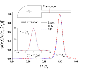
Figure 1: (color online). Focalization at the focal point for TRM (red dashed) and PIF (blue dotted) procedures contrasted with the exact reversal (solid). PIF and exact curves coincide for times close to $2t_{R}$. Top: basic scheme of a quantum bazooka device with a localized excitation inside. Left inset: spatial contrast in the recovered signal.

In the numerical solution, the propagation of an initial gaussian wave-packet with enegy $(k_{o}a)^{2}V$ is recorded by a single transducer placed in the waveguide consisting of a single propagating mode (in practice, this waveguide is well represented by a one-dimensional chain). The time evolution was performed through a second order Trotter-Suzuki algorithm DeRaedt . Fig.(1) shows the recovered signal at the focal point, i.e. the centroid of the original wave-packet. The focalization functions for both methods are close to the exact reversed propagation. However, a slight broadening of the focalized wave-packet is observed in the TRM. In this case, the differences between PIF and TRM procedures are small because the initial excitation is mainly composed by states whose group velocity in the outgoing channel remains almost constant.

II.2 PIF in a classical Helmholtz resonator

The PIF procedure for a classical wave equation can be readily deduced using our Green’s function strategy by considering its finite difference version. This is best visualized as a system of coupled oscillators Economou . By including an inhomogeneity, it becomes in a simple model for a Helmholtz resonator coupled to an acoustic waveguide. Here, the lowest frequency $\omega_{0}$ of the $\lambda/2$ mode in the resonator is represented by a single mass $m_{0}$ and its corresponding spring. The waveguide is modelled by a semi-infinite chain of identical masses $m=\alpha m_{0}$ placed at the equilibrium points $x_{n}=na$ (with $a$ the lattice constant and $n$ a positive integer). The nearest neighbor spring constant is $K=m\omega_{\mathrm{x}}^{2}$. The equations of motion for the corresponding displacements $u_{n}$ can be written in a matrix form which, in the frequency domain, reads:

$$\mathbb{D}^{-1}(\omega)\mathbf{u}(\omega)=\left(\begin{array}[]{ccc}\omega^{2}-\tilde{\omega}_{0}^{2}&\alpha\omega_{\mathrm{x}}^{2}&\cdots\\ \omega_{\mathrm{x}}^{2}&\omega^{2}-2\omega_{\mathrm{x}}^{2}&\\ \vdots&&\ddots\end{array}\right)\mathbf{u}(\omega)=0,$$ (31)

where $\tilde{\omega}_{0}^{2}=\omega_{0}^{2}+\alpha\omega_{\mathrm{x}}^{2}$. Here, $\mathbb{D(\omega)}$ represents a momentum-displacement response function, which is the resolvent of the dynamical matrix. Any diagonal element has a simple expression in terms of continued fractions. In particular, a far-field transducer is placed at the site $x_{s}$ on the waveguide, where the response function is

$$D_{s,s}(\omega)=\frac{1}{\omega^{2}-2\omega_{\mathrm{x}}^{2}-\Delta_{L}(\omega)-\left[\Delta_{R}(\omega)-\mathrm{i}\omega\eta(\omega)\right]}.$$ (32)

Here, the mean-field frequency $2\omega_{\mathrm{x}}^{2}$ appears shifted by the dynamical effect from the oscillators at both sides of $x_{s}$. The imaginary shift indicates that excitation components of different frequencies would eventually escape through the waveguide at the right with group velocities

$$v_{g}(\omega)=\frac{a}{2}\eta(\omega)=\frac{a}{2}\sqrt{4\omega_{\mathrm{x}}^{2}-\omega^{2}}.$$ (33)

The propagation of an excitation originated in the resonator $x_{0}$ is detected in $x_{s}$ inside the waveguide. The recorded signal presents a strong component in $\tilde{\omega}_{0}$, which is the “carrier” frequency as can be appreciated from the density of states at the resonator’s site. The displacement at the transducer, resulting from an initial excitation $\xi_{0}$ in the resonator, can be expressed as

$$u_{s}(t)=G_{s,0}(t)\xi_{0},\ t>0,$$ (34)

where $G_{s,0}(t)$ is the Green’s function describing the displacement-displacement response. In general, the connection between the Green’s function and the momentum-displacement response is given by

$$G_{i,j}(\omega)=\mathrm{i}\omega D_{i,j}(\omega).$$ (35)

As before, the complete evolution $\tilde{u}_{s}(t)$ in the transducer can be conceived as the forward evolution corresponding to the positive times and a backward evolution accounting for the negative ones. In this sense,

$$\tilde{u}_{s}(t)=\left\{\begin{array}[]{cc}u_{s}(-t),&t<0,\\ u_{s}(t),&t\geq 0,\end{array}\right.$$ (36)

and the injection that produces the desired reversion can be obtained as

$$\delta u_{s}(\omega)=\frac{\tilde{u}_{s}^{\ast}(\omega)}{G_{s,s}(\omega)}.$$ (37)

According to eq.(34), the complete evolution writes in the frequency domain as

$$\tilde{u}_{s}^{\ast}(\omega) =u_{s}^{\ast}(\omega)+u_{s}(\omega)$$ (38)

$$=\left[G_{s,0}^{\ast}(\omega)+G_{s,0}(\omega)\right]\Delta u_{0}.$$ (39)

Here again, the key tool is the Dyson equation connecting the two subspaces delimited by the transducer. We can write

$$G_{s,0}(\omega)=\frac{G_{s,s}(\omega)}{G_{s,s}^{\ast}(\omega)}G_{s,0}^{\ast}(\omega),$$ (40)

and the PIF injection rewrites in terms of the partial evolution corresponding to the detected signal

$$\delta u_{s}^{\mathrm{PIF}}(\omega) =\left[\frac{1}{G_{s,s}(\omega)}+\frac{1}{G_{s,s}^{\ast}(\omega)}\right]u_{s}^{\ast}(\omega)$$ (41)

$$=\frac{1}{\mathrm{i}\omega}\left[\frac{1}{D_{s,s}(\omega)}-\frac{1}{D_{s,s}^{\ast}(\omega)}\right]u_{s}^{\ast}(\omega)$$ (42)

$$=\eta(\omega)u_{s}^{\ast}(\omega).$$ (43)

As in the quantum case, we denote $2\omega_{\mathrm{x}}u_{s}^{\ast}(\omega)$ as the Fourier transform $\delta u_{s}^{\mathrm{TRM}}(\omega)$ of the injection function in the TRM protocol. In consequence, the perfect time reversal is obtained only once a further filter $v_{g}(\omega)/v_{\max}$ is applied. Hence, the PIF formula for internal source in the acoustic case is

$$\delta u_{s}^{\mathrm{PIF}}(\omega)=\frac{v_{g}(\omega)}{v_{\max}}\delta u_{s}^{\mathrm{TRM}}(\omega).$$ (44)

Notably, the prescription remains exactly the same as that of the quantum version (see eq.(30)). This implies that the effectiveness of the filter will depend on the structure of the waveguide and the initial wave-packet, regardless the details of the cavity. However, for cases in which the group velocity in the free space is constant, it is clear that $\delta u_{s}^{\mathrm{PIF}}(\omega)\equiv\delta u_{s}^{\mathrm{TRM}}(\omega)$.

A numerical simulation of the reconstruction of the initial excitation was performed using the Pair Partitioning method (PPM) CalvoMC , which yields the complete dynamics by alternating among the evolutions of pairs of coupled masses. In a similar way as the Trotter algorithm, PPM approximates the actual evolution determined by the Hamiltonian $H_{1}+H_{2}$ during a small time step $\delta t$ as a sequence of unitary transformations $U\left[(H_{1}+H_{2})\delta t\right]\simeq U\left[H_{1}\delta t\right]U\left[H_{2}\delta t\right]$ and results in a perfectly reversible algorithm. The calculated dynamics is best depicted, as in fig.(2), by analyzing the local energy which avoids the fast fluctuations shown by displacement and momentum. Here, the left panel shows (in a log scale) that the recovered resonator’s local energy coincides with the exact reversal over all the relevant ranges. Since in this model the waveguide has a cut-off frequency, as would be the case in a grated waveguide, the PIF filter improves the TRM focusing when it comes to reproduce the low intensity signals. This is particularly evident in the reproduction of the time-reversed survival collapse. This is a sudden dip in the local energy resulting from the interference between the excitation surviving in the resonator and that returning from the waveguide. This surprising phenomenom was originally described in the context of quantum spin channels Rufeil . The perfect contrast of the time reversed signal provided by PIF is evidenced in the right panel by the exact cancellation of displacements except for the resonator. It is also interesting to notice that both procedures produce a phantom signal outside the “silence region”. While the TRM has an evident imperfection in the localization of the signal, the PIF procedure yields this absolute cancellation even outside the cavity region defined by the far field transducer at $x_{s}$. The resulting localization, which corresponds to $\lambda/2$ of the carrier signal, was only enabled by filtering out the band edge components in the emitted signal. From this perspective, the PIF procedure contributes to the goal of achieving focusing beyond the diffraction limit FinkSCIENCE .

Figure 2: (color online). (a) Balls and springs model for a Helmholtz resonator coupled to a waveguide. (b) Focalization signal in the resonator. Left panel: local energy recovered as function of time. Both methods, the TRM (red dashed) and PIF (blue dotted) are contrasted with the exact reversal (solid). PIF and exact curves coincide for the whole temporal range. Right Panel: Displacements at the focalization time.

III Conclusions

We presented an expression of the PIF procedure which results particularly simple when the excitation is generated by an internal source. We observed that, contrary to what happens when the source is external, the prescription does not involve internal details of the cavity but only the simpler information about the propagation in the outer region. Hence, this filter applies to two physically relevant situations: 1) When the excitation is actually originated in the interior of the cavity. In this case, one obtains a perfect reversal of the wave function for all the times after the source has been turned-off. 2) When one uses an external source in a situation that allows for a clear separation between incoming and outgoing waves. In that case, one can use the recording of the outgoing wave to perfectly reverse the whole excursion of the excitation through the cavity. This condition is achieved when the boundaries are placed far enough from the reverberant region, as in the quantum and acoustic bazooka devices. An interesting consequence of our result in the acoustical case is that TRM produces a perfect time reversal within the cavity, provided that the propagation beyond its contour is free of further reverberances.

A numerical assesment of the reversion fidelity shows that PIF constitutes a notable improvement over TRM prescription in cases where the energy (frequency) dependence has a non-linear dispersion relation, as typical excitations described by the Schrödinger equation or, in acoustic systems, when the escape velocity is not constant. This occurs in the presence of multiple propagating channels or when collisions outside the cavity have a relevant contribution as in grated waveguides.

The PIF prescription becomes an analytical tool to design specific excitations well beyond the discussed TRM context, thus providing an alternative strategy for coherent control. In particular, it allows the design of quantum bazookas that shoot wave packet excitations. Feasible implementations of this concept include the local generation of vibrational waves in nanoelectromechanical structures Schwab . There, the excitation is injected through the coupling of a Cooper-pair box to a nanocantilever. In Bose-Einstein condensates confined to an optical lattice Chu , there is a well-defined set of quantum states with tunable couplings. Thus, the generation of macroscopic wavefunctions would benefit from our simple and consistent PIF prescription. Last but not least, in NMR, the injection of targeted spin-wave packets in chains of interacting spins Madi-Ernst is possible through the local injection of the polarization stored in a rare ${}^{13}C$ nucleus Alvarez .

- (1) Fink M., Sci. Am., 281 May issue (1999) 67.
- (2) Fink M., Montaldo G. and Tanter M., Annual Rev. Biomed. Eng., 5 (2003) 465.
- (3) Edelman G. F. et al., IEEE J. Ocean Eng., 27 (2002) 602.
- (4) Henty B. E. and Stancil D. D., Phys. Rev. Lett., 93 (2004) 243904.
- (5) Jalabert R. A. and Pastawski H. M., Phys. Rev. Lett., 86 (2001) 2490.
- (6) De Rosny J., Tourin A., Derode A., Roux P. and Fink M., Phys. Rev. Lett., 95 (2005) 074301.
- (7) Calvo H. L. and Pastawski H. M., Physica B, 398 (2007) 317.
- (8) Pastawski H. M., Danieli E. P., Calvo H. L. and Foa Torres L. E. F., EPL, 77 (2007) 40001 (5pp).
- (9) Kuperman W. A., J. Acoust. Soc. Am., 119 (2006) 2.
- (10) Tanter M., Thomas J-L. and Fink M., J. Acoust. Soc. Am., 108 (2000) 223.
- (11) Vignon F., de Rosny J., Aubry J-F. and Fink M., J. Acoust. Soc. Am., 122 (2007) 2715.
- (12) Lerosey G., de Rosny J., Tourin A. and Fink M., Science, 315 (2007) 1120.
- (13) Ulrich T. J., Johnson P. A. and Guyer R. A., Phys. Rev. Lett, 98 (2007) 104301.
- (14) Li X. and Stockman M. I., Phys. Rev. B, 77 (2008) 195109.
- (15) Calvo H. L., Jalabert R. A. and Pastawski H. M., Phys. Rev. Lett., 101 (2008) 240403.
- (16) Economou E. N., Green’s Functions in Quantum Physics, 3rd Ed.(Springer-Verlag, Heidelberg, 2006).
- (17) Pastawski H. M., Weisz J. F. and Albornoz S., Phys. Rev. B, 28 (1983) 2896.
- (18) Pastawski H. M., Foa Torres L. E. F. and Medina E., Chem. Phys., 281 (2002) 257.
- (19) Pastawski H. M. and Medina E., Rev. Mex. Fís., 47 (2001) 1.
- (20) De Raedt H., Ann. Rev. of Comp. Physics, IV (1996) 107.
- (21) Calvo H. L. and Pastawski H. M., Mec. Comp., XXVI (2007) 74.
- (22) Rufeil Fiori E. and Pastawski H. M., Chem. Phys. Lett., 420 (2006) 35.
- (23) Schwab K. C. and Roukes M. L., Phys. Today, 58 (7) (2005) 36.
- (24) Chu S., Nature, 416 (2002) 206.
- (25) Mádi Z. L. et al., Chem. Phys. Lett., 268 (1997) 300.
- (26) Alvarez G. A. et al., J. Chem. Phys., 124 (2006) 194507; Levstein P. R., Usaj G. and Pastawski H. M., ibid, 108 (1998) 2718.