Efficient Parallel and Out of Core Algorithms for Constructing Large Bi-directed de Bruijn Graphs

Abstract

Assembling genomic sequences from a set of overlapping reads is one of the most fundamental problems in computational biology. Algorithms addressing the assembly problem fall into two broad categories – based on the data structures which they employ. The first class uses an overlap/string graph and the second type uses a de Bruijn graph. However with the recent advances in short read sequencing technology, de Bruijn graph based algorithms seem to play a vital role in practice.

Efficient algorithms for building these massive de Bruijn graphs are very essential in large sequencing projects based on short reads. In [1], an $O(n/p)$ time parallel algorithm has been given for this problem. Here $n$ is the size of the input and $p$ is the number of processors. This algorithm enumerates all possible bi-directed edges which can overlap with a node and ends up generating $\Theta(n\Sigma)$ messages.

In this paper we present a $\Theta(n/p)$ time parallel algorithm with a communication complexity equal to that of parallel sorting and is not sensitive to $\Sigma$. The generality of our algorithm makes it very easy to extend it even to the out-of-core model and in this case it has an optimal I/O complexity of $\Theta(\frac{n\log(n/B)}{B\log(M/B)})$. We demonstrate the scalability of our parallel algorithm on a SGI/Altix computer. A comparison of our algorithm with that of [1] reveals that our algorithm is faster. We also provide efficient algorithms for the bi-directed chain compaction problem.

I Introduction

The genomic sequence of an organism is a string from the alphabet $\Sigma=\{A,T,G,C\}$. This string is also referred as the Deoxyribonucleic acid (DNA) sequence. DNA sequences exist as complementary pairs ($A-T$, $G-C$) due to the double strandedness of the underlying DNA structure. Several characteristics of an organism are encoded in its DNA sequence, thereby reducing the biological analysis of the organism to the analysis of its DNA sequence. Identifying the unknown DNA sequence of an organism is known as de novo sequencing and is of fundamental biological importance. On the other hand the existing sequencing technology is not mature enough to identify/read the entire sequence of the genome – especially for complex organisms like the mammals. However small fragments of the genome can be read with acceptable accuracy. The shotgun method employed in many sequencing projects breaks the genome randomly at several places and generates several small fragments (reads) of the genome. The problem of reassembling all the fragmented reads into a small sequence close to the original sequence is known as the Sequence Assembly (SA) problem.

Although the SA problem seems similar to the Shortest Common Super string (SCS) problem, there are in fact some fundamental differences. Firstly, the genome sequence might contain several repeating regions. However, in any optimal solution to the SCS problem we will not be able to find repeating regions – because we want to minimize the length of the solution string. In addition to the repeats, there are other issues such as errors in reads and double strandedness of the reads which make the reduction to SCS problem very complex.

The literature on algorithms to address the SA problem can be classified into two broad categories. The first class of algorithms model a read as a vertex in a directed graph – known as the overlap graph [2]. The second class of algorithms model every substring of length $k$ (i.e., a $k$-mer) in a read as a vertex in a (subgraph of) a de Bruijn graph [3].

In an overlap graph, for every pair of overlapping reads, directed edges are introduced consistent with the orientation of the overlap. Since the transitive edges in the overlap graph are redundant for the assembly process they are removed and the resultant graph is called the string graph [2]. The edges of the string graph are classified into optional, required and exact. The SA problem is reduced to the identification of a shortest walk in the string graph which includes all the required and exact constraints on the edges. Identifying such a walk – minimum $S$-walk – on the string graph is known to be NP-hard [4].

When a de Bruijn graph is employed, we model every substring of length $k$ (i.e., a $k$-mer) in a read as a vertex  [3]. A directed edge is introduced between two $k$-mers if there exists some read in which these two $k$-mers overlap by exactly $k-1$ symbols. Thus every read in the input is mapped to some path in the de Bruijn graph. The SA problem is reduced to a Chinese Postman Problem (CPP) on the de Bruijn graph, subject to the constraint that the resultant CPP tour include all the paths corresponding to the reads. This problem is also known to be NP-hard. Thus solving the SA problem exactly on both these graph models is intractable.

Overlap graph based algorithms were found to perform better (see  [5] [6] [7] [8]) with Sanger based read methods. Sanger methods produce reads typically around $1000$ base pairs long. However these can produce significant read errors. To overcome the issues with Sanger reads new read technologies such as the pyrosequencing (454sequencing) have emerged. These read technologies can produce reliable and accurate genome fragments which are very short (up to $100$ base-pairs long). On the other hand short read technologies can increase the number of reads in the SA problem by a large magnitude. Overlap based graph algorithms do not scale well in practice since they represent every read as a vertex. De Bruijn graph based algorithms seem to handle short reads very efficiently (see [9]) in practice compared to the overlap graph based algorithms. However the existing sequential algorithms [9] to construct these graphs are sub-optimal and require significant amounts of memory. This limits the applicability of these methods to large scale SA problems. In this paper we address this issue and present algorithms to construct large de Bruijn graphs very efficiently. Our algorithm is optimal in the sequential, parallel and out-of-core models. A recent work by Jackson and Aluru [1] yielded parallel algorithms to build these de Bruijn graphs efficiently. They present a parallel algorithm that runs in $O(n/p)$ time using $p$ processors (assuming that $n$ is a constant-degree ploynomial in $p$). The message complexity of their algorithm is $\Theta(n\Sigma)$. By message complexity we mean the total number of messages (i.e., $k$-mers) communicated by all the processors in the entire algorithm. One of the major contributions of our work is to show that we can accomplish this in $\Theta(n/p)$ time with a message complexity of $\Theta(n)$. An experimental comparison of these two algorithms on an SGI Altix machine shows that our algorithm is considerably faster. In addition, our algorithm works optimally in an out-of-core setting. In particular, our algorithm requires only $\Theta(\frac{n\log(n/B)}{B\log(M/B)})$ I/O operations.

The organization of the paper is as follows. In Section II we introduce some preliminaries and define a bi-directed de Bruijn graph formally. Section III discusses our main algorithm in a sequential setting. Section V and Section VI show how our main idea can easily be extended to parallel and out-of-core models optimally. In Section V-A we provide some remarks on the parallel algorithm of Jackson and Aluru [1]. Section VII gives algorithms to perform the simplification operation on the bi-directed de Bruijn graph. Section VIII discusses how our simplified bi-directed de Bruijn graph algorithm can replace the graph construction algorithm in a popular sequence assembly program VELVET [9]. Finally we present experimental results in Section IX.

II Preliminaries

Let $s\in\Sigma^{n}$ be a string of length $n$. Any substring $s_{j}$ (i.e., $s[j]s[j+1]\ldots s[j+k-1],n-k+1\geq j\geq 1$) of length $k$ is called a $k-$mer of $s$. The set of all $k-$mers of a given string $s$ is called the $k-$spectrum of $s$ and is denoted by $\mathbb{S}(s,k)$. Given a $k-$mer $s_{j}$, $\bar{s_{j}}$ denotes the reverse complement of $s_{j}$ (e.g., if $s_{j}=AAGTA$ then $\bar{s_{j}}=TACTT$). Let $\leq$ be the partial ordering among the strings of equal length, then $s_{i}\leq s_{j}$ indicates that the string $s_{i}$ is lexicographically smaller than $s_{j}$. Given any $k-$mer $s_{i}$, let $\hat{s_{i}}$ be the lexicographically smaller string between $s_{i}$ and $\bar{s_{i}}$. We call $\hat{s_{i}}$ the canonical $k-$mer of $s_{i}$. In other words, if $s_{i}\leq\bar{s_{i}}$ then $\hat{s_{i}}=s_{i}$ otherwise $\hat{s_{i}}=\bar{s_{i}}$. A $k-$molecule of a given $k-$mer $s_{i}$ is a tuple $(\hat{s_{i}},\bar{\hat{s_{i}}})$ consisting of the canonical $k-$mer of $s_{i}$ and the reverse complement of the canonical $k-$mer. In the rest of this paper we use the terms positive strand and canonical $k-$mer interchangeably. Likewise the non-canonical $k-$mer is referred to as the negative strand.

A bi-directed graph is a generalized version of a standard directed graph. In a directed graph every edge has only one arrow head ($\text{--}\rhd$ or $\lhd\text{--}$). On the other hand in a bi-directed graph every edge has two arrow heads attached to it ($\lhd\text{--}\rhd$, $\lhd\text{--}\lhd$,$\rhd\text{--}\lhd$ or $\rhd\text{--}\rhd$). Let $V$ be the set of vertices and $E=\{(v_{i},v_{j},o_{1},o_{2})|v_{i},v_{j}\in V\wedge o_{1},o_{2}\in\{\lhd,\rhd\}\}$ be the set of bi-directed edges in a bi-directed graph $G(V,E)$. For any edge $e=(v_{i},v_{u},o_{1},o_{2})\in E$, $o_{1}=e[o^{+}]$ and $o_{2}=e[o^{-}]$ refer to the orientations of the arrow heads on the vertices $v_{i}$ and $v_{j}$, respectively. A walk $W(v_{i},v_{j})$ between two nodes $v_{i},v_{j}\in V$ of a bi-directed graph $G(V,E)$ is a sequence $v_{i},e_{i_{1}},v_{i_{1}},e_{i_{2}},v_{i_{2}},\ldots,v_{i_{m}},e_{i_{m+1}},v_{j}$, such that for every intermediate vertex $v_{i_{l}},1\leq l\leq m$ the orientation of the arrow head on the incoming edge adjacent on $v_{i_{l}}$ is opposite to the orientation of the arrow head on the out going edge. To make this clearer, let $e_{i_{l}},v_{i_{l}},e_{i_{l+1}}$ be a sub-sequence in the walk $W(v_{i},v_{j})$. If $e_{i_{l}}=(v_{i_{l-1}},v_{i_{l}},o_{1},o_{2}),e_{i_{l+1}}=(v_{i_{l}},v_{i_{l+1}},o_{1}^{\prime},o_{2}^{\prime})$ then for the walk to be valid it should be the case that $o_{2}\neq o_{1}^{\prime}$. Figure 1$(a)$ illustrates an example of a bi-directed graph. Figure 1$(b)$ shows a simple bi-directed walk between the nodes $A$ and $E$. Bi-directed walk between two nodes may not be simple. Figure 1$(c)$ shows a bi-directed walk between $A$ and $E$ which is not simple – because $B$ repeats twice.

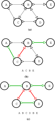
Figure 1: Bi-directed graph and bi-directed walks

A de Bruijn graph $D^{k}(s)$ of order $k$ on a given string $s$ is defined as follows. The vertex set $V$ of $D^{k}(s)$ is defined as the $k-$spectrum of $s$ (i.e. $V=\mathbb{S}(s,k)$). We use the notation $suf(v_{i},l)$ ($pre(v_{i},l)$, respectively) to denote the suffix (prefix, respectively) of length $l$ in the string $v_{i}$. Let the symbol $\circ$ denote the concatenation operation between two strings. The set of directed edges $E$ of $D^{k}(s)$ is defined as follows: $E=\{(v_{i},v_{j})|suf(v_{i},k-1)=pre(v_{j},k-1)\wedge v_{i}[1]\circ suf(v_{i},k-1)\circ v_{j}[k]\in\mathbb{S}(s,k+1)\}$. We can also define de Bruijn graphs for sets of strings as follows. If $S=\{s_{1},s_{2}\ldots s_{n}\}$ is any set of strings, a de Bruijn graph $B^{k}(S)$ of order $k$ on $S$ has $V=\displaystyle\cup_{i=1}^{n}\mathbb{S}(s_{i},k)$ and $E=\{(v_{i},v_{j})|suf(v_{i},k-1)=pre(v_{j},k-1)\wedge\exists\,l:v_{i}[1]\circ suf(v_{i},k-1)\circ v_{j}[k]\in\mathbb{S}(s_{l},k+1)\}$. To model the double strandedness of the DNA molecules we should also consider the reverse complements ($\bar{S}=\{\bar{s_{1}},\bar{s_{2}}\ldots\bar{s_{n}}\}$) while we build the de Bruijn graph.

To address this a bi-directed de Bruijn graph $BD^{k}(S\cup\bar{S})$ has been suggested in  [4]. The set of vertices $V$ of $BD^{k}(S\cup\bar{S})$ consists of all possible $k-$molecules from $S\cup\bar{S}$. The set of bi-directed edges for $BD^{k}(S\cup\bar{S})$ is defined as follows. Let $x,y$ be two $k-$mers which are next to each other in some input string $z\in S\cup\bar{S}$. Then an edge is introduced between the $k-$molecules $v_{i}$ and $v_{j}$ corresponding to $x$ and $y$, respectively. Please note that two consecutive $k-$mers in some input string always overlap by $k-1$ symbols. The converse need not be true. The orientations of the arrow heads on the edges are chosen as follows. If both $x$ and $y$ are the positive strands in $v_{i}$ and $v_{j}$, respectively, then an edge $(v_{i},v_{j},\rhd,\rhd)$ is introduced. If $x$ is the positive strand in $v_{i}$ and $y$ is the negative strand in $v_{j}$ an edge $(v_{i},v_{j},\rhd,\lhd)$ is introduced. Finally, if $x$ is the negative strand in $v_{i}$ and $y$ is the positive strand in $v_{j}$ an edge $(v_{i},v_{j},\lhd,\rhd)$ is introduced.

Figure 2 illustrates a simple example of the bi-directed de Bruijn graph of order $k=3$ from a set of reads $ATGG,CCAT,GGAC,GTTC,TGGA$ and $TGGT$ observed from a DNA sequence $ATGGACCAT$ and its reverse complement $ATGGTCCAT$. Consider two $3-$molecules $v_{1}=(GGA,TCC)$ and $v_{2}=(GAC,GTC)$. Because the positive strand $x=GGA$ in $v_{1}$ overlaps the positive strand $y=GAC$ in $v_{2}$ by string $GA$, an edge $(v_{1},v_{2},\rhd,\rhd)$ is introduced. Note that the negative strand $GTC$ in $v_{2}$ also overlaps the negative strand $TCC$ in $v_{2}$ by string $TC$, so the two overlapping strings $GA$ and $TC$ are drawn above the edge $(v_{1},v_{2},\rhd,\rhd)$ in Figure 2. A bi-directed walk on the example bi-directed de Bruijn graph as illustrated by the dash line is corresponding to the original DNA sequence with the first letter omitted $TGGACCAT$. We would like to remark that the parameter $k$ is always chosen to be odd to ensure that the forward and reverse complements of a $k$-mer are not the same.

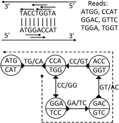
Figure 2: Bi-directed de Bruijn graph example

III Our algorithm to construct bi-directed de Bruijn graphs

In this section we describe our algorithm BiConstruct to construct a bi-directed de Bruijn graph on a given set of reads. The following are the main steps in our algorithm to build the bi-directed de Bruijn graph. Let $R_{f}=\{r_{1},r_{2}\ldots r_{n}\},r_{i}\in\Sigma^{r}$ be the input set of reads. $\bar{R_{f}}=\{\bar{r_{1}},\bar{r_{2}}\ldots\bar{r_{n}}\}$ is a set of reverse complements. Let $R^{*}=R_{f}\cup\bar{R_{f}}$ and $R^{k+1}=\displaystyle\cup_{r\in R^{*}}\mathbb{S}{(r,k+1)}$. $R^{k+1}$ is the set of all $(k+1)$-mers from the input reads and their reverse complements.

• [STEP-1] Generate canonical edges: Let $(x,y)=(z[1\ldots k],z[2\ldots k+1])$ be the $k-$mers corresponding to a $(k+1)$-mer $z[1\ldots k+1]\in R^{k+1}$. Recall that $\hat{x}$ and $\hat{y}$ are the canonical $k-$mers of $x$ and $y$, respectively. Create a canonical bi-directed edge $(\hat{v_{i}},\hat{v_{j}},o_{1},o_{2})$ for each $(k+1)$-mer as follows.

  $$\begin{array}[]{l}(\hat{v_{i}},\hat{v_{j}},o_{1},o_{2})=\left\{\begin{array}[]{lr}&\text{$x=\hat{x},y=\hat{y}$}\\ (\hat{x},\hat{y},\rhd,\rhd)&\text{IF $\hat{x}\leq\hat{y},$}\\ (\hat{y},\hat{x},\lhd,\lhd)&\text{ELSE}\\ &\\ &\text{$x\neq\hat{x}\wedge y=\hat{y}$}\\ (\hat{x},\hat{y},\lhd,\rhd)&\text{IF $\hat{x}\leq\hat{y}$}\\ (\hat{y},\hat{x},\lhd,\rhd)&\text{ELSE}\\ &\\ &\text{$x=\hat{x}\wedge y\neq\hat{y}$}\\ (\hat{x},\hat{y},\rhd,\lhd)&\text{IF $\hat{x}\leq\hat{y}$}\\ (\hat{y},\hat{x},\rhd,\lhd)&\text{ELSE}\\ &\\ &\text{$x\neq\hat{x}\wedge y\neq\hat{y}$}\\ (\hat{x},\hat{y},\lhd,\lhd)&\text{IF $\hat{x}\leq\hat{y},$}\\ (\hat{y},\hat{x},\rhd,\rhd)&\text{ELSE}\\ \end{array}\right.\end{array}$$

• [STEP-2] Reduce multiplicity: Sort all the bi-directed edges in [STEP-1], using radix sort. Since the parameter $k$ is always odd this guarantees that a pair of canonical $k$-mers have exactly one orientation. Remove the duplicates and record the multiplicities of each canonical edge. Gather all the unique canonical edges into an edge list $\mathcal{E}$.

• [STEP-3] Collect bi-directed vertices: For each canonical bi-directed edge $(\hat{v_{i}},\hat{v_{j}},o_{1},o_{2})\in\mathcal{E}$, collect the canonical $k$-mers $\hat{v_{i}}$, $\hat{v_{j}}$ into list $\mathcal{V}$. Sort the list $\mathcal{V}$ and remove duplicates, such that $\mathcal{V}$ contains only the unique canonical $k$-mers.

• [STEP-4] Adjacency list representation: The list $\mathcal{E}$ is the collection of all the edges in the bi-directed graph and the list $\mathcal{V}$ is the collection of all the nodes in the bi-directed graph. It is now easy to use $\mathcal{E}$ and generate the adjacency lists representation for the bi-directed graph. This may require one extra radix sorting step.

IV Analysis of the algorithm BiConstruct

Theorem 1

Algorithm BiConstruct builds a bi-directed de Bruijn graph of the order $k$ in $\Theta(n)$ time. Here $n$ is number of characters/symbols in the input.

Proof:

Without loss of generality assume that all the reads are of the same size $r$. Let $N$ be the number of reads in the input. This generates a total of $(r-k)N$ $(k+1)$-mers in [STEP-1]. The radix sort needs to be applied at most $2k\log(|\Sigma|)$ passes, resulting in $2k\log(|\Sigma|)(r-k)N$ operations. Since $n=Nr$ is the total number of characters/symbols in the input, the radix sort takes $\Theta(kn\log(|\Sigma|))$ operations assuming that in each pass of sorting only a constant number of symbols are used. If $k\log(|\Sigma|)=O(\log N)$, the sorting takes only $O(n)$ time. In practice since $N$ is very large in relation to $k$ and $|\Sigma|$, the above condition readily holds. Since the time for this step dominates that of all the other steps, the runtime of the algorithm BiConstruct is $\Theta(n)$. ∎

V Parallel algorithm for building bi-directed de Bruijn graph

In this section we illustrate a parallel implementation of our algorithm. Let $p$ be the number of processors available. We first distribute $N/p$ reads for each processor. All the processors can execute [STEP-1] in parallel. In [STEP-2] we need to perform parallel sorting on the list $\mathcal{E}$. Parallel radix/bucket sort –which does not use any all-to-all communications– can be employed to accomplish this. For example, the integer sorting algorithm of Kruskal, Rudolph and Snir takes $O\left(\frac{n}{p}\frac{\log n}{\log(n/p)}\right)$ time. This will be $O(n/p)$ if $n$ is a constant degree polynomial in $p$. In other words, for coarse-grain parallelism the run time is asymptotically optimal. In practice coarse-grain parallelism is what we have. Here $n=N(r-k+1)$. We call this algorithm Par-BiConstruct.

Theorem 2

Algorithm Par-BiConstruct builds a bi-directed de Bruijn graph in time $O(n/p)$. The message complexity is $O(n)$.

V-A Some remarks on Jackson and Aluru’s algorithm

The algorithm of Jackson and Aluru [1] first identifies the vertices of the bi-directed graph – which they call representative nodes. Then for every representative node $|\Sigma|$ many-to-many messages were generated. These messages correspond to potential bi-directed edges which can be adjacent on that representative node. A bi-directed edge is successfully created if both the representatives of the generated message exist in some processor, otherwise the edge is dropped. This results in generating a total of $\Theta(n|\Sigma|)$ many-to-many messages. The authors in the same paper demonstrate that communicating many-to-many messages is a major bottleneck and does not scale well. On the other had we remark that the algorithm BiConstruct does not involve any many-to-many communications and does not have any scaling bottlenecks.

On the other hand the algorithm presented in their paper [1] can potentially generate spurious bi-directed edges. According to the definition [4] of the bi-directed de Bruijn graph in the context of SA problem, a bi-directed edge between two $k$-mers/vertices exists iff there exists some read in which these two $k$-mers are adjacent. We illustrate this by a simple example. Consider a read $r_{i}=AATGCATC$. If we wish to build a bi-directed graph of order $3$, then $\{AAT,ATG,TGC,GCA,CAT,ATC\}$ form a subset of the vertices of the bi-directed graph. In this example we see that $k$-mers $AAT$ and $ATC$ overlap by exactly $2$ symbols. However there cannot be any bi-directed edge between them according to the definition – because they are not adjacent. On the other hand the algorithm presented in  [1] generates the following edges with respect to $k$-mer $AAT$: $\{(AAT,ATA),(AAT,ATG),(AAT,ATT)$, $(AAT,ATC)\}$. The edges $(AAT,ATA)$ and $(AAT,ATC)$ are purged since the $k$-mers $ATA$ and $ATC$ are missing. However bi-directed edges with corresponding orientations are established between $ATG$ and $ATC$. Unfortunately $(AAT,ATC)$ is a spurious edge and can potentially generate wrong assembly solutions. In contrast to their algorithm [1] our algorithm does not use all-to-all communications – although we use point-point communications.

VI Out of core algorithms for building bi-directed de Bruijn graphs

Theorem 3

There exists an out-of core algorithm to construct a bi-directed de Bruijn graph using an optimal number of I/O’s.

Proof:

Sketch: Replace the radix sorting with an external $R-$way merge which takes only $\Theta(\frac{n\log(n/B)}{B\log(M/B)})$. Where $M$ is the main memory size, $n$ is the sum of the lengths of all reads, and $B$ is the block size of the disk. ∎

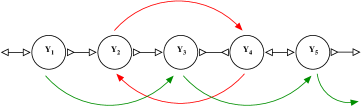
Figure 3: Problems with pointer jumping on bi-directed chains

VII Simplified bi-directed de Bruijn graph

The bi-directed de Bruijn graph constructed in the previous section may contain several linear chains. These chains have to be compacted to save space as well as time. The graph that results after this compaction step is refered to as the simplified bi-directed graph. A linear chain of bi-directed edges between nodes $u$ and $v$ can be compacted only if we can find a valid bi-directed walk connecting $u$ and $v$. All the $k$-mers/vertices in a compactable chain can be merged into a single node, and relabelled with the corresponding forward and reverse complementary strings. In Figure 4 we can see that the nodes $X_{1}$ and $X_{3}$ can be connected with a valid bi-directed walk and hence these nodes are merged into a single node. In practice the compaction of chains seems to play a very crucial role. It has been reported that merging the linear chains can reduce the number of nodes in the graph by up-to $30\%$ [9].

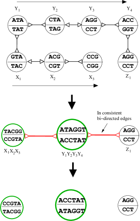
Figure 4: Issues with partially compacted bi-directed chains

Figure 5: Transforming bi-directed chain compaction to list ranking

Although bi-directed chain compaction problem seems like a list ranking problem there are some fundamental differences. Firstly, a bi-directed edge can be traversed in both the directions. As a result, applying pointer jumping directly on a bi-directed graph can lead to cycles and cannot compact the bi-directed chains correctly. Figure 3 illustrates the first phase of pointer jumping. As we can see, the green arcs indicate valid pointer jumps from the starting nodes. However since the orientation of the node $Y_{4}$ is reverse relative to the direction of pointer jumping a cycle results. In contrast, a valid bi-directed chain compaction would merge all the nodes between $Y_{1}$ and $Y_{5}$ since there is a valid bi-directed walk between $Y_{1}$ and $Y_{5}$. On the other hand, bi-directed chain compaction may result in inconsistent bi-directed edges and these edges should be recognised and removed. Consider a bi-directed chain in Figure 4; this chain contains two possible bi-directed walks – $Y_{1}$ to $Y_{4}$ and $X_{1}$ to $X_{3}$. The walk from $Y_{1}$ to $Y_{4}$ ($Y_{4}$ to $Y_{1}$) spells out a label $ATAGGT$($ACCTAT$) after compaction. Once we perform this compaction the edge between $Y_{4}$ and $Z_{1}$ in the original graph is no longer valid – because the $k$-mer on $Z_{1}$ cannot overlap with the label $ACCTAT$. The same is true for the compaction of the bi-directed walk between $X_{1}$ and $X_{3}$. The redundant edges after compaction are marked in red. Since bi-directed chain compaction has a lot of practical importance efficient and correct algorithms are essential.

We now provide algorithms for the bi-directed chain compaction problem. Our key idea here is to transform a bi-directed graph into a directed graph and then apply list ranking. Given a list of candidate canonical bi-directed edges, we apply a ListRankingTransform (see Figure 5) which introduces two new nodes $v^{+},v^{-}$ for every node $v$ in the original graph. Directed edges corresponding to the orientation are introduced. See Figure 5.

Lemma 1

Let $BG(V,E)$ be a bi-directed graph; let $BG^{t}(V^{t},E^{t})$ be the directed graph after applying ListRankingTransform. Two nodes $u,v\in V$ are connected by a bi-directed path iff $u^{+}\in V^{t}$ ($u^{-}\in V^{t}$) is connected to one of $v^{+}$($v^{-}$) or $v^{-}$($v^{+}$) by a directed path.

Proof:

We first prove the forward direction by induction on the number of nodes in the bi-directed graph. Consider the basis of induction when $|V|=2$, let $v_{0},v_{1}\in V$. Clearly we are only interested when $v_{0}$ and $v_{1}$ are connected by a bi-directed edge. By the definition of ListRankingTransform the Lemma in this case is trivially true. Now consider a bi-directed graph with $|V|=n+1$ nodes, if the path between $v_{i},i<n$ and $v_{j},j<n$ does not involve node $v_{n}$ the lemma still holds by induction on the sub bi-directed graph $BG(V-\{v_{n}\},E)$. Now assume that $v_{i}\ldots v_{p},v_{n},v_{q}\ldots v_{j}$ is the bi-directed path between $v_{i}$ and $v_{j}$ involving the node $v_{n}$; see Figure 6(a). Also Figure 6(a) shows how the transformed directed graph look like; observe the colors of bi-directed edges and corresponding directed edges. By induction hypothesis on the sub bi-directed paths $v_{i}\ldots v_{p},v_{n}$ and $v_{n},v_{q}\ldots v_{j}$ we have the following. $v_{i}^{+}$ is connected to $v_{n}^{+}$ or $v_{n}^{-}$ by some directed path $P_{1}$ (See Figure 6(b); $v_{n}^{+}$ is connected to $v_{j}^{+}$ or $v_{j}^{-}$ by some directed path $P_{2}$. We examine three possible cases depending on how the directed edge from $P_{1}$ and $P_{2}$ is incident on $v_{n}^{+}$. In CASE-1 we have both $P_{1}$ and $P_{2}$ pointing into node $v_{n}^{+}$. This implies that the orientation of the bi-directed edges in the original graph is according to Figure 6(b). In this case we cannot have a bi-directed walk involving the node $v_{n}$, which contradicts our original assumption. Similarly CASE-2(Figure 6(c)) would also lead to a similar contradiction. Only CASE-3 would let node $v_{n}$ involve in a bi-directed walk. In this case $v_{i}^{+}$ will be connected to either $v_{j}^{+}$ or $v_{j}^{-}$ by concatenation of the paths $P_{1},P_{2}$. We can make a similar argument to prove the reverse direction. ∎

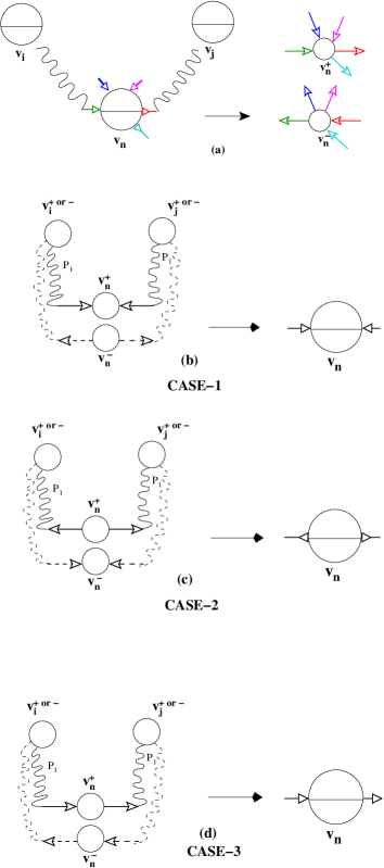
Figure 6: Proof that ListRankingTransform preserves bi-directed walk in the original graph.

VII-A Algorithm for bi-directed chain compaction

We first identify a set of candidate bi-directed edges which can potentially form a chain. One possible criterion will be to include all the edges which are adjacent on bi-directed nodes with exactly one in and out degree. Each candidate bi-directed edge is transformed using ListRankingTranform and list ranking is applied on resultant set. As a consequence of the symmetry in ListRankingTransform we would see both forward and reverse complements of the compacted chains in the output. We can further canonicalize each chain and remove the duplicates by sorting. This results in unique bi-directed chains from the candidate bi-directed edges. Finally we report only the chains which are resultant of compaction of at least three bi-directed nodes. This removes all the inconsistent edges (see Figure 4) from further consideration. As a consequence of Lemma 1 all the bi-directed chains are correctly compacted.

VII-B Analysis of bi-directed compaction on parallel and out-of-core models

Let $\mathcal{E}_{l}$ be the list of candidate edges for compaction. To do compaction in parallel, we can use a Segmented Parallel Prefix on $p$ processors to accomplish this in time $O(|2\mathcal{E}_{l}|/p+\log(p))$. On the other hand list ranking can also be done out-of-core as follows. Without loss of generality we can treat the input for the list ranking problem as a set $S$ of ordered tuples of the form $(x,y)$. Given $S$ we create a copy and call it $S^{\prime}$. We now perform an external sort of $S$, $S^{\prime}$ with respect to $y$ (i.e., using the $y$ value of tuple $(x,y)$ as the key) and $x$ respectively. The two sorted lists are scanned linearly to identify tuples $(x,y)\in S$, $(x^{\prime},y^{\prime})\in S^{\prime}$ such that $y=x^{\prime}$. These two tuples are merged into a single tuple $(x,y^{\prime})$ and are added to a list $\mathcal{E}^{\prime}_{l}$. This process is now repeated on $\mathcal{E}^{\prime}_{l}$. Note that if the underlying graph induced by $\mathcal{E}_{l}$ does not have any cycles then $|\mathcal{E}^{\prime}_{l}|\leq|\mathcal{E}_{l}|/2$; which means that the size of $\mathcal{E}^{\prime}_{l}$ geometrically decreases after every iteration. The I/O complexity of each iteration is dominated by the external sorting and hence bi-directed compaction can be accomplished out-of-core with $\Theta(|\mathcal{E}_{l}|/B\log_{\frac{M}{B}}(|\mathcal{E}_{l}|/B))$ I/O operations.

Care should be taken to deal with cycles. There are two ways of dealing with cycles. One way is to first identify all the cycles in the bi-directed graph (generated in the previous section) and then break these cycles by removing appropriate edges. A second easy is to identify the cycles on the fly and break them. We employ the second approach.

VIII Improving the construction of the bi-directed de Bruijn graph in some practical assemblers

In this section we briefly describe how our algorithms can be used to speedup some of the existing SA programs. As an example, we consider VELVET [9]. VELVET is a suite of programs – velveth and velvetg, which has recently gained acclamation in assembling short reads. VELVET program builds a simplified bi-directed graph from a set of reads. We now briefly describe the algorithm used in VELVET to build this graph. VELVET program puts all the $k$-mers from the input into a hash table and then identifies the $k$-mers which are present in at least 2 reads – this information is called the roadmap in VELVET’s terminology. The program then builds a de Bruijn graph using these $k$-mers. Finally it takes every read and threads it on these $k$-mers. The worst case time complexity is $O(n\log(n))$ – assuming that $k$ and $|\Sigma|$ are constants. On the other hand since VELVET builds this graph entirely in-memory, this has some serious scalability problems especially on large scale assembly projects. However VELVET seems to have some very good assembly heuristics to remove errors and identify redundant assembly paths, etc. Thus our algorithm can act as a replacement to code in VELVET which performs in-memory graph construction.

IX Experimental results

We have compared the performance of our algorithm and that of Jackson and Aluru [1]. We refer to the later algorithm as JA. To make this comparison fair, we have implemented the JA algorithm also on the same platform that our algorithm runs on. We have used a SGI/Altix IA-64 machine with 64 nodes for all of our experiments. Our implementation uses MPI for communication between the processors. Table I shows the user and system times for both our algorithm and the JA algorithm. We can clearly see that the system time (communication time) is consistently higher for the JA algorithm. Also, as we move from one million to eight million reads the increase in the system time is quite significant for the JA algorithm (e.g., the system time for JA increases from 0.621 sec to 4.120 sec, which is almost a 7X increase. On the other hand there is only a 3X increase in our algorithm). The JA algorithm has a higher communication cost because it enumerates all the bi-directed edges and uses many-to-many messages to send to the right processor.

The user time of our algorithm is also consistently superior compared to the user time of JA. This clearly is because we do much less local computations. In contrast, JA needs to do a lot of local processing which arises from processing all the received edges, removing redundant ones, and collecting the necessary edges to perform many-to-many communications. Since JA was taking a significant amount of time on for inputs larger than 8 million we have compared these algorithms only for input sizes up to 8 million. The experimental results reported in [1] start with at least 64 processors. We however show the scalablity of our algorithm upto $128$ million reads in Table II. Table II clearly demonstrates the scalability of our algorithm. We make our implementations available at http://trinity.engr.uconn.edu/~vamsik/ParBidirected.tgz.

p	JA ALGO		OUR ALGO
	user time	sys time	user time	sys time	speed up
	(sec)	(sec)	(sec)	(sec)
READS=$1048576$
4	55.932	0.621	2.365	0.046	23.456
8	25.161	0.331	3.072	0.035	8.205
16	13.603	0.175	0.619	0.038	20.971
32	5.711	0.157	0.149	0.099	23.661
READS=$8388608$
4	593.712	4.120	20.807	0.159	28.514
8	341.694	2.322	17.637	0.105	19.390
16	147.629	1.117	17.734	0.087	8.347
32	72.413	0.566	13.967	0.120	5.181

TABLE I: Comparision between the JA algorithm and our algorithm

p	user time	sys time	wall time
	(ticks)	(ticks)	(min:sec)
READS=$16777216$
2	37147	259	1:14.02
4	37254	85	0:38.95
8	20217	57	0:21.90
16	16951	55	0:19.73
32	12901	40	0:16.38
READS=$33554432$
2	148070	1219	2:42.66
4	99067	677	1:48.60
8	47319	322	0:55.41
16	17936	135	0:25.64
32	9973	191	0:17.55
READS=$67108864$
2	340653	2348	6:18.77
4	240861	1931	4:14.57
8	153782	1781	2:39.18
16	64408	804	1:10.91
32	46659	486	0:53.32
READS=$134217728$
2	770922	5560	15:00.42
4	471196	4272	8:29.62
8	314281	3456	5:17.65
16	135562	2148	2:21.83
32	82414	950	1:28.87

TABLE II: Scalablility of our algorithm for up to 128 million reads

X Conclusions

In this paper we have presented an efficient algorithm to build a bi-directed de Bruijn graph which is a fundamental data structure for any sequence assembly program – based on Eulerian approach. Our algorithms are also efficient in parallel and out of core settings. These algorithms can be used in building large scale bi-directed de Bruijn graphs. Also, our algorithm does not employ any all-to-all communications in parallel setting and performs better than that of Jackson and Aluru [1].

Acknowledgements. This work has been supported in part by the following grants: NSF 0326155, NSF 0829916 and NIH 1R01GM079689-01A1.

References

- [1] B. G. Jackson and S. Aluru, “Parallel construction of bidirected string graphs for genome assembly,” 2008, pp. 346–353.
- [2] J. D. Kececioglu and E. W. Myers, “Combinatorial algorithms for dna sequence assembly,” Algorithmica, vol. 13, no. 1-2, pp. 7–51, 1995.
- [3] P. A. Pevzner, H. Tang, and M. S. Waterman, “An eulerian path approach to dna fragment assembly,” Proceedings of the National Academy of Sciences of the United States of America, vol. 98, no. 17, pp. 9748–9753, 2001.
- [4] P. Medvedev, K. Georgiou, G. Myers, and M. Brudno, Computability of models for sequence assembly, 2007, vol. 4645 LNBI.
- [5] X. Huang, J. Wang, S. Aluru, S. . Yang, and L. Hillier, “Pcap: A whole-genome assembly program,” Genome research, vol. 13, no. 9, pp. 2164–2170, 2003, cited By (since 1996): 61. [Online]. Available: www.scopus.com
- [6] E. W. Myers, G. G. Sutton, A. L. Delcher, I. M. Dew, D. P. Fasulo, M. J. Flanigan, S. A. Kravitz, C. M. Mobarry, K. H. J. Reinert, K. A. Remington, E. L. Anson, R. A. Bolanos, H. . Chou, C. M. Jordan, A. L. Halpern, S. Lonardi, E. M. Beasley, R. C. Brandon, L. Chen, P. J. Dunn, Z. Lai, Y. Liang, D. R. Nusskern, M. Zhan, Q. Zhang, X. Zheng, G. M. Rubin, M. D. Adams, and J. C. Venter, “A whole-genome assembly of drosophila,” Science, vol. 287, no. 5461, pp. 2196–2204, 2000.
- [7] S. Batzoglou, D. B. Jaffe, K. Stanley, J. Butler, S. Gnerre, E. Mauceli, B. Berger, J. P. Mesirov, and E. S. Lander, “Arachne: A whole-genome shotgun assembler,” Genome research, vol. 12, no. 1, pp. 177–189, 2002.
- [8] “Phrap assembler,” [http://www.phrap.org/].
- [9] D. R. Zerbino and E. Birney, “Velvet: Algorithms for de novo short read assembly using de bruijn graphs,” Genome research, vol. 18, no. 5, pp. 821–829, 2008.