Discreteness-Induced Slow Relaxation in Reversible Catalytic Reaction Networks
Abstract
Slowing down of the relaxation of the fluctuations around equilibrium is investigated both by stochastic simulations and by analysis of Master equation of reversible reaction networks consisting of resources and the corresponding products that work as catalysts. As the number of molecules is decreased, the relaxation time to equilibrium is prolonged due to the deficiency of catalysts, as demonstrated by the amplification compared to that by the continuum limit. This amplification ratio of the relaxation time is represented by a scaling function as , and it becomes prominent as becomes less than a critical value , where is the inverse temperature and is the energy gap between a product and a resource.
I I. Introduction
The study of reaction processes in catalytic reaction networks is generally important to understand the dynamics and fluctuations in biochemical systems and their functionality. Obviously, understanding the generic features of equilibrium characteristics and relaxation to equilibrium is the first step toward gaining such an understanding. Indeed, such reaction systems often exhibit anomalous slow relaxation to equilibrium due to some kinetic constraints such as diffusion-influenced (limited) reactionDLR and formations of transient Turing patternsAK2 . In this paper, we consider a novel mechanism to realize such slow relaxation in catalytic reaction networks, where the discreteness in molecule number that may reach zero induces drastic slowing down.
Most intra-cellular reactions progress with the aid of catalysts (proteins), whereas catalysts have to be synthesized as a result of such catalytic reactions. Indeed, reaction dynamics in catalytic networks have been extensively investigated. In most such studies, a limiting case with a strong non-equilibrium condition was assumed by adopting a unidirectional reaction process (i.e., by neglecting backward reactions). To understand the basic properties of biochemical reactions, however, it is important to study both equilibrium and non-equilibrium characteristics by including forward and backward reactions that satisfy the detailed balance condition. Such a study is not only important for statistical thermodynamics but it also provides some insight on the regulation of synthesis or degradation reactions for homeostasis in cells.
Recently, we discovered a slow relaxation process to equilibrium, which generally appears in such catalytic reaction networks, and proposed ”chemical-net glass” as a novel class of nonequilibrium phenomena. In this case, relaxation in the vicinity of equilibrium is exponential, whereas far from it, much slower logarithmic relaxation with some bottlenecks appears due to kinetic constraints in catalytic relationshipsAK3 . In this study, we adopted continuous rate equations and assumed that the molecule number is sufficiently large.
In biochemical reaction processes, however, some chemical species can play an important role at extremely low concentrations of even only a few molecules per cellcell2 ; cell3 ; cell4 . In such systems, fluctuations and discreteness in the molecule number are important. Indeed, recent studies by using a stochastic simulation of catalytic reaction networks have demonstrated that the smallness in the molecule number induces a drastic change with regard to statistical and spatiotemporal behaviors of molecule abundances from those obtained by the rate equation, i.e., at the limit of large molecule numberstogashi1 ; ookubo ; AK1 ; AK11 ; mif1 ; mif2 ; Solomon ; togashi3 ; marion ; zhdanov ; Dau ; Kaneko-Adv ; Furusawa ; Furusawa2 . In these studies, the strong nonequilibrium condition is assumed by taking a unidirectional reaction.
Now, it is important to study the relaxation process to equilibrium by considering the smallness in the molecule number. Does the discreteness in molecule number influence the equilibrium and relaxation behaviors? Is the relaxation process slowed down by the smallness in the molecule number? To address this question, we have carried out several simulations of the relaxation dynamics of random catalytic reaction networks by using stochastic simulations. Numerical results from several networksSAK1 ; SAK2 suggest that the relaxation time is prolonged drastically when the number of molecules is smaller. The increase from the continuum limit is expressed by the factor , where is the additional energy required to pass through the bottleneck due to the discreteness in molecule number and is the inverse temperature.
In this paper, we analyze such slowing down of a reaction process to equilibrium that is induced by the smallness in molecule numbers. Instead of taking complex reaction networks, we choose simple networks or network motives to estimate the relaxation time analytically. In fact, complex networks are often constructed by combining a variety of simple network motives with simple branch or loop structures. We focus on the relaxation dynamics of reversible catalytic reaction systems with such simple network motives as a first step toward understanding the general relaxation properties in complex catalytic reaction networks.
In section II, we introduce two network motives, where the synthesis of a product from resource molecules (and its reverse reaction) is catalyzed by one of the other products. Here, we note that some specific network motives may exhibit incomplete equilibration when the molecule number decreases, and the average chemical concentration in the steady state deviates from the equilibrium concentration derived by the continuous rate equations.
In section III, we show relaxation characteristics from the stochastic simulations. The relaxation of the fluctuation around the steady state slows down as the molecule number is decreased below a critical value. This increase is represented by a scaling function by using , where is the molecule number and , the energy gap between a product and a resource. In section IV, we present an analytic estimate for this relaxation suppression due to the smallness in molecule number by using a suitable approximation for Master equation. In section V, we present a summary and discuss the generality of our results.
II II. Models
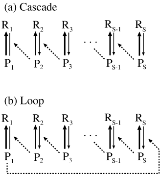
Here, we consider reversible catalytic reaction systems with two simple network structures, cascade system and loop system, as shown in Fig. 1, which may function as network motives for complex reaction networks. These systems consist of chemical species, which are Product and Resource with . Here, each product chemical can catalyze at most one of the other Resource-Product reactions, whereas each reaction is catalyzed at most by some product. (Instead, we can interpret that there exist chemical species with excited and non-excited states, and chemicals in an excited state can catalyze an excitation reaction of one of the other molecules.)
If all chemicals are catalyzed by one of them, we can renumber and for and write the reaction as
,
where , which leads to the loop system (b). When there
exist a reaction that is not catalyzed, the cascade system in
Fig.1a) is obtained where
.
(Neglecting cases in which some pair of resource and product is
totally disconnected from others, the loop and cascade systems are
the only possibilities).
The rates of forward () and backward () reactions are set so that they satisfy the detailed balance condition. We assume that the energy of the chemical is larger than that of , and we set and , where is the energy gap between and and is the inverse temperature. We define and as the number of molecules of the chemical species and , respectively. We fix the total number of molecules as , and holds for each . The state of the system is represented by a set of numbers .
In both the systems, it is noted that for (i.e., the continuous limit), and holds at the equilibrium distribution, which is reached at .
For finite , however, there is a difference between the distribution of the cascade and the loop systems. In the cascade system, the average of the equilibrium chemical concentrations are identical to the continuum limit, and are given by , that is, they are independent of and . This is because all the states () are connected by reactions and the above equilibrium distribution is only the stationary solution for Master equation.
On the other hand, in the loop system, there is a deviation in the steady chemical concentration from the continuum limit, which becomes more prominent as becomes smaller. This is because the state cannot be reached from other states, whereas the state cannot move to any other states. Hence, the steady distribution from the initial conditions without deviates from the continuum limit. This deviation becomes prominent as becomes smaller. For example, for and , the distribution from the initial condition without is given by . Note that tends to with an increase in .
III III. Simulation results
In this section, we present the results of stochastic simulations and show the dependence of the relaxation process on the number of molecules and the inverse temperature . For simplicity, we consider to be uniform for all species (); however, this assumption can be relaxed.
Numerical simulations are carried out by iterating the following stochastic processes. (i) We randomly pick up a pair of molecules, say, molecule 1 and 2. (ii) Molecule 1 is transformed with its reaction rate (if it is P, it is transformed to R, and vice versa) if molecule 2 can catalyze the reaction of molecule 1. In the cascade case, there is a reaction that progresses without a catalyst, and in this case, if molecule 1 is the one that reacts without a catalyst, then it is transformed with the reaction rate independently of 2. Here, a unit time is defined as the time span in which the above processes for catalytic reactions are repeated times. In each unit time, each molecule is picked up on average to check if the transformation occurs.
In the following, we focus on the behavior of the system after a sufficiently long time from the initial time where the numbers of each molecule and are set randomly from under the constraint and .
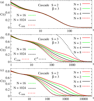
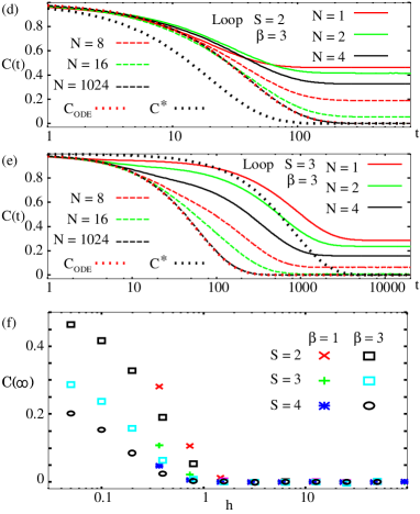
Figure 2(a)-2(e) show the auto-correlation functions of the deviation from the equilibrium concentration of the cascade system ((a)-(c)) and the loop system ((d) and (e)) for some and N with , defined by and . As already discussed, in the cascade system whereas for small . The value starts to deviate when becomes less than 1. Hence, we have plotted of the loop system as a function of in Fig.2(f) for and . As shown, holds for independently of . On the other hand, in both systems, the relaxation to the final state with for small is drastically slowed down as compared to that for large when , whereas the relaxation for small is faster when .
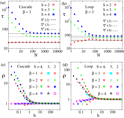
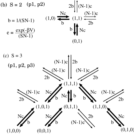
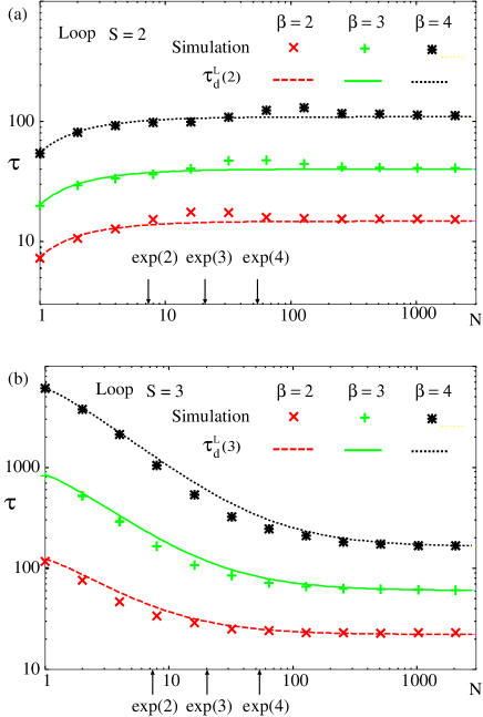
To observe the dependence of the relaxation time on , we measured the integrated relaxation time defined as . Figure 3(a) and (b) show as a function of for with for the (a) cascade system and (b) loop system. For , the relaxation time increases by several orders of magnitude with a decrease in in both systems. On the other hand, for does not exhibit any drastic change with the decrease in in both systems.
This prolongation of for becomes more prominent as is increased. From several data, is suggested to increase as a function of ). Combining and dependencies, we introduce a parameter . The discreteness effect is dominant when is less than unity. Figure 3(c) and 3(d) show as a function of for the (c) cascade system and (d) loop system for several values of and . For , the deviation of from the continuum limit () becomes prominent when is below unity in both systems. The increase in appears to become steeper with an increase in . On the other hand, for does not exhibit a drastic increase with a decrease in .
IV IV. Origin of slow relaxations and crossover
IV.1 A. Relaxation processes for and
Now, we analytically estimate the enhancement in relaxation time and explain its representation in the form . For this purpose, we compare the estimate by Master equation analysis for small and compare it with that from the continuum limit .
In the continuum limit, the reaction dynamics are represented by the following rate equation:
| (1) |
with . Here, for in the cascade system and for in the loop system. In both systems, holds for . When the deviation from equilibrium is small, its evolution for the loop systems obeys the following linearized equation
| (2) |
For the cascade system, this equation is also valid for the elements , whereas . Then, the auto-correlation function of a small fluctuation of around is obtained as
| (3) |
for the loop system, and
| (4) |
for the cascade system. Indeed, these agree quite well with the simulation results for a sufficiently large (e.g., in Fig. 2.). Thus, the characteristic time of the relaxation is estimated as for the loop system and for the cascade system, which are consistent with the simulation results shown in Fig. 3.
As the other extreme limit, consider the case with . In this case, the relaxation dynamics are dominated by a completely different process induced by the absence of catalysts whose number can often go to zero. In such cases, states are trapped at some local energy minimum that appears due to the deficiency of catalysts. Then, the hopping processes among them play an important role in the relaxation dynamics, as shown below. In the following, we focus the cases with and to clarify that such an effect is induced by discreteness in the molecule number. Note that, as shown in the last section, the behavior for is distinct from that for ; in the former case, the relaxation time is enhanced by the decrease in , in contrast to the latter case.
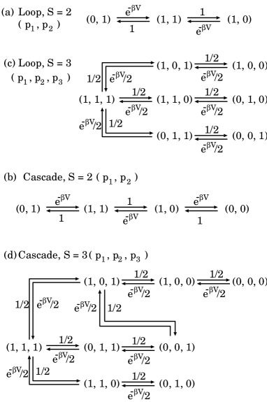
First, we study the loop system. When , the system realizes 3 states from the initial conditions—, , and —as shown in Fig. 4(a). Then, we estimate the time of the transition between and . First, the transition rate from the state to is estimated as follows: for this transition, a pair of molecules from the product of the first species and the resource of the second species has to be chosen. This probability is given by , while the reaction rate is given by . Hence the rate is given by . Thus, the characteristic time of the correlation of each is given by , which is consistent with the results shown in Fig. 2(d).
On the other hand, for , the system realizes 7 states—, , ,, , , and —as shown in Fig. 4(b). The characteristic time of the correlation of each is given by the transition time among the three branches including lowest-energy states, - , - , and - . Here, in order to hop from one branch to another, the system must go through the highest-energy state , due to the restriction by the catalytic relation. Now, we define the probability that the states in the branch - are realized as . Then, the probability to realize the state is given by . Here, the transition rate from to is given by . Then, the probability current from the the branch - is estimated by (). Because of the symmetry among the catalytic reactions, the probability currents from the other branches are obtained in the same way, to get the same form. Thus, the escape rate from each branch is estimated by , and the characteristic time of the correlation of each is estimated as . Because the relaxation time in the continuum limit is proportional to , the deviation from it increases with , which is consistent with the results shown in Fig. 2(e). Thus, the enhancement of the relaxation time from the continuous case is explained.
Essentially the same argument is also valid for the cascade systems. When , the system can realize transitions among 4 states——as shown in Fig. 4(c). Here, is a metastable state and is the lowest-energy state. The relaxation is characterized by the escape rate from a metastable state, which is given by . Thus, the characteristic time of the correlation of each is given by .
On the other hand, for , the system realizes 8 states–, , , ,, , , and —as shown in Fig. 4(d). The slowest characteristic time of the relaxation is given by the transition time from the branch, - since the system must go through the highest-energy state , which is a limiting process for this case. Then, in a manner similar to the loop system with , the characteristic time is obtained as . This gives the characteristic time of the slowest motions of the system. This estimation fits well with the numerical result shown in Fig. 2(b).
IV.2 B. , dependencies of and relaxation time
Next, we extend the argument of the last subsection to analyze the and dependencies of and the relaxation time in greater detail. In particular, we explain why gives a critical value and how the amplification of relaxation time depends on for . Because of the simplicity due to the symmetry in the catalytic relationship, we only study loop systems; however, the argument presented below can be extended to cascade systems.
Figure 5(a) shows the transition diagram of the loop system with , where each circle indicates each state and the arrows indicate possible transitions. Generally, for any values of , the transition rate from a state to a state per unit time is estimated as follows. For this transition, a pair of molecules from the resource of the th species () and the product of the th species () has to be chosen. This probability is given by , and the reaction rate is given by . Hence, the transition rate per unit time is given by . Similarly, the transition rate in the opposite direction is given as . If the molecule number is so large or is so small that , holds for small and holds for large . Then, the dominant states of the system are located in an intermediate region in the phase space . For example, the blue region in Fig. 5(a) indicates such dominant states for .
Now, we define the probability that as , and the joint probability to realize and as . Here, and . Then the time evolution of follows
| (5) |
Then, we obtain
| (6) |
where (). Using this equation, we obtain the time evolution of as
| (7) |
This implies that obeys equation (1) for a sufficiently large value of .
On the other hand, if is so small or is so large that , holds for all and . Thus, for all tend to decrease to . Then, there exist metastable states—, , … , , … , and (). Among them, the following states, , , …, and , have the lowest energy. For example, in the cases with , the states and () are metastable states and and are the lowest-energy states.
It should be noted that the lowest-energy states are the dominant states for . The probability to realize these lowest-energy states tends to with an increase in . Thus, with the increase in , approaches for small , which indicates for small and large .
Moreover, for , the transitions among lowest-energy states contribute dominantly to the relaxation process. Then, we estimate the characteristic time of the fluctuations of the system for by considering the transition processes from one lowest-energy states such as to the other lowest-energy states such as . In the following, we consider only the cases with and . We only focus on the dynamics of under the constraint that has only or , because .
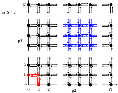
First, consider the case with . Figure 5(b) shows a detailed transition diagram around the region where () are only or . The escape rate from and are given by . Thus, the characteristic time of the correlation of each is given by
| (8) |
which is consistent with the results shown in Fig. 6(a).
Next, we study the case with . The transition diagram of the states is shown in Fig.5(c) when () take only or . Similar to the case, the characteristic time of the transition among the three branches including lowest-energy states, - , - , and - through the state is considered. In a manner similar to the case, the transition rate from each branch is estimated by . Thus, the relaxation time of the fluctuation of is estimated as the decrease with as
| (9) |
Considering the dependence of , the above estimate is consistent with Fig. 6(b).
For larger than , the transition diagram becomes rather complicated. However, a similar analysis should be possible to estimate the prolongation in the relaxation time.
V V. Summary and discussions
In the present paper, the slowing down of the relaxation in reversible catalytic reaction networks induced by the smallness of molecule number is investigated as a general property of catalytic reaction networks. This prolongation of relaxation is a result of bottlenecks in reactions; these appear due to the deficiency of the catalyst required for a reaction. The number of molecules can be so small that the number of catalysts becomes zero. In this case, a pair of a substrate and the corresponding catalyst molecule species can hardly exist simultaneously. Such a constraint makes it difficult to realize a specific configuration necessary for the relaxation. The probability for realization is given by , with as the corresponding energy barrier to realize such rare conditions, or the sum of such energy barriers. This bottleneck energy is generally different from the energy gap in the continuum limit that is obtained from the rate equation (ordinary differential equation). Thus, the relaxation time at a small molecule number deviates from the continuum case by the factor with an appropriate effective energy difference, .
By considering the models of simple catalytic reaction networks consisting of resource chemicals of species and the corresponding products, we have demonstrated this deviation of relaxation time from both direct simulations and analysis by using Master equation. From the numerical and analytic estimates, and for , where is the energy gap between the resource and the product chemicals. For , in general, the prolongation of the relaxation time becomes prominent when is less than unity, and its amplification ratio from the continuum limit is represented as a function of and . Note that the cascade system in the case is equivalent to the ”Asymmetrically Constrained Ising Chain” (ACIC), Hierarchically constrained Ising model, or East model, which are studied as simple abstract models for glassy statesaici_1 ; aici_2 ; aici_3 . Following the interpretation therein, the increase in relaxation time at as a result of the decrease in or temperature may be regarded as a type of glass transition. According to the recent studies on ACIC, the correlation time of the motion of (not the relaxation time of the total system) is estimated as where the integer obeys aici_2 ; aici_3 . In cases with , this fact is consistent with our estimate of the relaxation time of the cascade system with . The estimation of as a function of and for general cases both for cascade and loop systems is an important issue that should be studied in the future.
In addition to the slow down in relaxation, the equilibrium distribution deviates in a network called a loop system, where all the reactions are catalyzed by one of the products. The constraint that the numbers of a certain pair of chemical species cannot simultaneously be zero leads to the deviation of the average distribution of molecule numbers from the continuum limit. Again, this deviation becomes prominent when is less than unity.
Although we have adopted simple network motives to analyze the relaxation, the prolongation of relaxation time is quite general in catalytic reaction networks. Catalytic bottlenecks often appear as the number of molecules is decreased in a large variety of reaction networks in which catalysts are synthesized withinSAK1 ; SAK2 . The present study can provide a basis for the general case with complex networks, as the motives here are sufficiently small and can exist within such complex networks.
Biochemical reactions generally progress in the presence of catalysts that are themselves synthesized as products of such reactions. These reactions form a network of a variety of chemical species. Here, the molecule number of each species is generally not very large. Hence, the slow relaxation process and deviation from equilibrium discussed in this study may underlie intracellular reaction processes. Moreover, the present network motives are so simple that they are suggested to exist in biochemical networks. We also note that the resource and product in our model can be interpreted as non-excited and excited states of enzymatic molecules. Indeed, many molecules are known to exhibit catalytic activity only when they are in an excited state, which can help other chemicals to switch to an excited state. In fact, such networks with mutual excitation are known in signal-transduction networkssig1 ; sig2 ; sig3 , where the present slow relaxation mechanism may be relevant to sustain the excitability of a specific enzyme type over a long time span. It is important to pursue the relevance of the present mechanism in cell-biological problems by considering more realistic models in the future.
We also note that not only the discreteness in the molecule number but also the negative correlation between a substrate and the corresponding catalyst within a reaction network or in a spatial concentration pattern suppresses the relaxation processAK2 ; AK3 ; SAK1 ; SAK2 . The present mechanism due to discreteness may work synergetically with the earlier mechanism to further suppress the relaxation to equilibrium. The construction of reaction networks to achieve slower relaxation together with the network analysis will be an important issue in the future.
The authors would like to Shinji Sano, for informing us of his finding on the prolongation of relaxation in reaction networks due to the discreteness in molecule numbers, which triggers the present study. A. A. was supported in part by a Grant-in Aid for Young Scientists (B) (Grant No. 19740260).
References
- (1) K. Kang, and S. Render, Phys. Rev. Lett 52, 955 (1984); M. Yamg, S. Lee, and K. J. Shin, Phys. Rev. Lett 79, 3783 (1997); I. V. Gopich, A. A. Ovchinnikov, and A. Szabo, Phys. Rev. Lett 86, 922 (2001); D. Pines, and E. Pines, J. Chem. Phys. 115, 951 (2001).
- (2) A. Awazu, and K. Kaneko, Phys. Rev. Lett 92, 258302 (2004).
- (3) A. Awazu, and K. Kaneko, Phys. Rev. E 80, 041931 (2009).
- (4) N. Olsson, E. Piek, P. ten Dijke, and G. Nilsson, J. Leuko. Biol. 67, 350 (2000).
- (5) P. Guptasarma, BioEssays 17, 987 (1995) .
- (6) H. H. McAdams, and A. Arkin, Trends Genet. 15, 65 (1999).
- (7) Y. Togashi, and K. Kaneko, Phys. Rev. Lett. 86, 2459 (2001); J. Phys. Soc. Jpn. 72, 62 (2003); J. Phys. Cond. Matt. 19, 065150 (2007).
- (8) J. Ohkubo, N. Shnerb, and D. A. Kessler, J. Phys. Soc. Jpn. 77, 044002 (2008).
- (9) A. Awazu, and K. Kaneko, Phys. Rev. E 76, 041915 (2007).
- (10) A. Awazu, and K. Kaneko, Phys. Rev. E 80, (2009) 010902(R).
- (11) B. Hess, and A. S. Mikhailov, Science 264, 223 (1994); J. Theor. Biol 176 181 (1995).
- (12) P. Stange, A. S. Mikhailov, and B. Hess, J. Phys. Chem B 104, 1844 (2000).
- (13) N. M. Shnerb, Y. Louzoun, E. Bettelheim, and S. Solomon, Proc. Nat. Acad. Sci. 97, 10322 (2000).
- (14) Y. Togashi, and K. Kaneko, Physica D 205, 87 (2005).
- (15) G. Marion, X. Mao, E. Renshaw, and J. Liu, Phys. Rev. E 66, 051915 (2002).
- (16) V. P. Zhdanov, Eur. Phys. J. B 29, 485 (2002).
- (17) T. Dauxois, F. D. Patti, D. Fanelli, and A. J. McKane, Phys. Rev. E 79, 036112 (2009)
- (18) K. Kaneko, Adv. Chem. Phys. 130, 543 (2005).
- (19) C. Furusawa, and K. Kaneko, Phys. Rev. Lett. 90, 088102 (2003).
- (20) C. Furusawa, et al., Biophysics 1, 25 (2005).
- (21) S.Sano, Master Thesis, Univ. of Tokyo, 2009 (in Japanese)
- (22) S. Sano, A. Awazu, and K. Kaneko, in preparation.
- (23) J. Jckle, and S. Eisinger, Z. Phys. B: Condens. Matter 84, 115 (1991).
- (24) F. Mauch, and J. Jckle, Physica A 262, 98 (1999).
- (25) P. Solich, and M. R. Evance, Phys. Rev. Lett. 83, 3238 (1999); Phys. Rev. E 68, 031504 (2003)
- (26) A. Goldbeter and D. K. Koshland, Jr., Proc. Nat. Acad. Sci. 78, 6840 (1981); J. Biol. Chem. 259, 4441 (1984).
- (27) A. Levchenko and P.A. Iglesias, Biophysical Journal 82, 50 (2002).
- (28) W. Ma, A. Trusina, H. El-Samad, W.A. Lim and C. Tang, Cell 138, 760 (2009).