Sparse Legendre expansions via $\ell_{1}$-minimization

Abstract

We consider the problem of recovering polynomials that are sparse with respect to the basis of Legendre polynomials from a small number of random samples. In particular, we show that a Legendre $s$-sparse polynomial of maximal degree $N$ can be recovered from $m\asymp s\log^{4}(N)$ random samples that are chosen independently according to the Chebyshev probability measure $d\nu(x)=\pi^{-1}(1-x^{2})^{-1/2}dx$. As an efficient recovery method, $\ell_{1}$-minimization can be used. We establish these results by verifying the restricted isometry property of a preconditioned random Legendre matrix. We then extend these results to a large class of orthogonal polynomial systems, including the Jacobi polynomials, of which the Legendre polynomials are a special case. Finally, we transpose these results into the setting of approximate recovery for functions in certain infinite-dimensional function spaces.

Key words: Legendre polynomials, sparse recovery, compressive sensing, $\ell_{1}$-minimization, condition numbers, random matrices, orthogonal polynomials.

AMS Subject classification: 41A10, 42C05, 94A20, 42A61, 60B20, 15A12, 65F35, 94A12.

1 Introduction

Compressive sensing has triggered significant research activity in recent years. Its central motif is that sparse signals can be recovered from what was previously believed to be highly incomplete information [10, 20]. In particular, it is now known [10, 13, 35, 30, 31, 32] that an $s$-sparse trigonometric polynomial of maximal degree $N$ can be recovered from $m\asymp s\log^{4}(N)$ sampling points. These $m$ samples can be chosen as a random subset from the discrete set $\{j/N\}_{j=0}^{N-1}$ [10, 13, 35], or independently from the uniform measure on $[0,1]$, see [30, 31, 32].

Until now, all sparse recovery results of this type required that the underlying basis be uniformly bounded like the trigonometric system, so as to be incoherent with point samples [11]. As the main contribution of this paper, we show that this condition may be relaxed, obtaining comparable sparse recovery results for any basis that is bounded by a square-integrable envelope function. As a special case, we focus on the Legendre system over the domain $[-1,1]$. To account for the blow-up of the Legendre system near the endpoints of its domain, the random sampling points are drawn according to the Chebyshev probability measure. This aligns with classical results on Lagrange interpolation which support the intuition that Chebyshev points are much better suited for the recovery of polynomials than uniform points are [8].

In order to deduce our main results we establish the restricted isometry property (RIP) for a preconditioned version of the matrix whose entries are the Legendre polynomials evaluated at sample points chosen from the Chebyshev measure. The concept of preconditioning seems to be new in the context of compressive sensing, although it has appeared within the larger scope of sparse approximation in a different context in [36]. It is likely that the idea of preconditioning can be exploited in other situations of interest as well.

Sparse expansions of multivariate polynomials in terms of tensor products of Legendre polynomials recently appeared in the problem of numerically solving stochastic or parametric PDEs [16, 3]. Our results indeed extend easily to tensor products of Legendre polynomials, and the application of our techniques in this context of numerical solution of SPDEs seems very promising. Our results may also be transposed into the setting of function approximation. In particular, we show that the aforementioned sampling and reconstruction procedure is guaranteed to produce near-optimal approximations to functions in infinite-dimensional spaces of functions having $\ell_{p}$-summable Fourier-Legendre coefficients ($0<p<1$), provided that the maximal polynomial degree in the $\ell_{1}$-reconstruction procedure is fixed appropriately in terms of the sparsity level.

Our original motivation for this work was the recovery of sparse spherical harmonic expansions [4] from randomly located samples on the sphere. While our preliminary results in this context seem to be only suboptimal [34], the results in the present paper apply at least to the recovery of functions on the sphere that are invariant under rotations of the sphere around a fixed axis. Sparse spherical harmonic expansions were recently exploited with good numerical success in the spherical inpainting problem for the cosmic microwave background [1], but so far this problem had lacked a theoretical understanding.

We note that the Legendre polynomial transform has fast algorithms for matrix vector multiplication; see for instance [28, 27, 17, 29, 39]. This fact is of crucial importance in numerical algorithms used for reconstructing the original function from its sample values – especially when the dimension of the problem gets large.

Our results extend to any polynomial system which is orthogonal with respect to a finitely-supported weight function satisfying a mild continuity condition; this includes the Jacobi polynomials, of which the Legendre polynomials are a special case. It turns out that the Chebyshev measure is universal for this rich class of orthogonal polynomials, in the sense that our corresponding result requires the random sampling points to be drawn according to the Chebyshev measure, independent of the particular weight function.

Our paper is structured as follows: Section 2 contains the main results for recovery of Legendre-sparse polynomials. Section 3 illustrates these results with numerical experiments. In Section 4 we recall known theorems on $\ell_{1}$-minimization and in Section 5, we prove the results presented in Section 2. Section 6 extends the results to a rich class of orthogonal polynomial systems, including the Jacobi polynomials, while Section 7 contains our main result on the recovery of continuous functions that are well approximated by Legendre-sparse polynomials.

Notation.

Let us briefly introduce some helpful notation. The $\ell_{p}$-norm on ${\mathbb{R}}^{N}$ is defined as $\|z\|_{p}=\Big{(}\sum_{j=1}^{N}|z_{j}|^{p}\Big{)}^{1/p},1\leq p<\infty,$ and $\|z\|_{\infty}=\max_{j=1,\ldots,N}|z_{j}|$ as usual. The “$\ell_{0}$-norm”, $\|z\|_{0}=\#\{j:z_{j}\neq 0\}$, counts the number of non-zero entries of $z$. A vector $z$ is called $s$-sparse if $\|z\|_{0}\leq s$, and the error of best $s$-term approximation of a vector $z\in{\mathbb{R}}^{N}$ in $\ell_{p}$ is defined as

$$\sigma_{s}(z)_{p}=\inf_{y:\|y\|_{0}\leq s}\|y-z\|_{p}.$$

Clearly, $\sigma_{s}(z)_{p}=0$ if $z$ is $s$-sparse. Informally, $z$ is called compressible if $\sigma_{s}(z)_{1}$ decays quickly as $s$ increases. A result due to Stechkin, see e.g. [21, Lemma 3.1], states that, for $q<p$,

$$\sigma_{s}(x)_{p}\leq s^{1/p-1/q}\|x\|_{q};$$ (1)

thus, vectors $x\in B_{q}^{N}=\{x\in{\mathbb{R}}^{N},\|x\|_{q}\leq 1\}$ for $0<q\leq 1$ can be considered a good model for compressible signals.

For $N\in{\mathbb{N}}$, we use the notation $[N]=\{1,\ldots,N\}$. In this article, $C>0$ will always denote a universal constant that might be different in each occurence.

The Chebyshev probability measure (also referred to as arcsine distribution) on $[-1,1]$ is given by $d\nu(x)=\pi^{-1}(1-x^{2})^{-1/2}dx$. If a random variable $X$ is uniformly distributed on $[0,\pi]$, then the random variable $Y=\cos{X}$ is distributed according to the Chebyshev measure.

2 Recovery of Legendre-sparse polynomials from a few samples

Consider the problem of recovering a polynomial $g$ from $m$ sample values $g(x_{1}),\ldots,g(x_{m})$. If the number of sampling points is less than or equal to the degree of $g$, such reconstruction is impossible in general due to dimension reasons. Therefore, as usual in the compressive sensing literature, we make a sparsity assumption. In order to introduce a suitable notion of sparsity we consider the basis of Legendre polynomials $L_{n}$ on $[-1,1]$, normalized so as to be orthonormal with respect to the uniform measure on $[-1,1]$, i.e. $\frac{1}{2}\int_{-1}^{1}L_{n}(x)L_{\ell}(x)dx=\delta_{n,\ell}$.

An arbitrary real-valued polynomial $g$ of degree $N-1$ can be expanded in terms of Legendre polynomials

$$g(x)=\sum_{n=0}^{N-1}c_{n}L_{n}(x),\quad x\in[-1,1].$$ (2)

If the coefficient vector $c\in{\mathbb{R}}^{N}$ is $s$-sparse, we call the corresponding polynomial Legendre $s$-sparse, or simply Legendre-sparse. If $\sigma_{s}(c)_{1}$ decays quickly as $s$ increases, then $g$ is called Legendre–compressible.

We aim to reconstruct Legendre–sparse polynomials, and more generally Legendre–compressible polynomials, of maximum degree $N-1$ from $m$ samples $g(x_{1}),\ldots,g(x_{m})$, where $m$ is desired to be small – at least smaller than $N$. Writing $g$ in the form (2) this task clearly amounts to reconstructing the coefficient vector $c\in{\mathbb{R}}^{N}$.

To the set of $m$ sample points $(x_{1},\hskip 2.84526pt\ldots\hskip 2.84526pt,x_{m})$ we associate the $m\times N$ Legendre matrix $\Phi$ defined component-wise by

$$\Phi_{j,k}=L_{k-1}(x_{j}),\quad j\in[m],\hskip 5.69054ptk\in[N].$$ (3)

Note that the samples $y_{j}=g(x_{j})$ may be expressed concisely in terms of the coefficient vector $c\in\mathbb{R}^{N}$ according to

$$y=\Phi c.$$

Reconstructing $c$ from the vector $y$ amounts to solving this system of linear equations. As we are interested in the underdetermined case $m<N$, this system typically has infinitely many solutions, and our task is to single out the original sparse $c$. The obvious but naive approach for doing this is by solving for the sparsest solution that agrees with the measurements,

$$\min_{z\in{\mathbb{R}}^{N}}\|z\|_{0}\quad\mbox{subject to}\quad\Phi z=y.$$ (4)

Unfortunately, this problem is NP-hard in general [18, 2]. To overcome this computational bottleneck the compressive sensing literature has suggested various tractable alternatives [25, 10, 38], most notably $\ell_{1}$-minimization (basis pursuit) [14, 10, 20], on which we focus in this paper. Nevertheless, it follows from our findings that greedy algorithms such as CoSaMP [38] or Iterative Hard Thresholding [7] may also be used for reconstruction.

Our main result is that any Legendre $s$-sparse polynomial may be recovered efficiently from a number of samples $m\asymp s\log^{3}(s)\log(N)$. Note that at least up to the logarithmic factors, this rate is optimal. Also the condition on $m$ is implied by the simpler one $m\asymp s\log^{4}{N}$ Reconstruction is also robust: any polynomial may be recovered efficiently to within a factor of its best approximation by a Legendre $s$-sparse polynomial, and, if the measurements are corrupted by noise, $g(x_{1})+\eta_{1},\ldots,g(x_{m})+\eta_{m}$, to within an additional factor of the noise level $\varepsilon=\|\eta\|_{\infty}$. We have

Theorem 2.1.

Let $N,m,s\in{\mathbb{N}}$ be given such that

$$m\geq Cs\log^{3}(s)\log(N).$$

Suppose that $m$ sampling points $(x_{1},\ldots,x_{m})$ are drawn independently at random from the Chebyshev measure, and consider the $m\times N$ Legendre matrix $\Phi$ with entries $\Phi_{j,k}=L_{k-1}(x_{j})$, and the $m\times m$ diagonal matrix ${\cal A}$ with entries $a_{j,j}=(\pi/2)^{1/2}(1-x_{j}^{2})^{1/4}$. Then with probability exceeding $1-N^{-\gamma\log^{3}(s)}$ the following holds for all polynomials $g(x)=\sum_{k=0}^{N-1}c_{k}L_{k}(x)$. Suppose that noisy sample values $y=\big{(}g(x_{1})+\eta_{1},\ldots,g(x_{m})+\eta_{m}\big{)}=\Phi c+\eta$ are observed, and $\|{\cal A}\eta\|_{\infty}\leq\varepsilon$. Then the coefficient vector $c=(c_{0},c_{1},\ldots,c_{N-1})$ is recoverable to within a factor of its best $s$-term approximation error and to a factor of the noise level by solving the inequality-constrained $\ell_{1}$-minimization problem

$$c^{\#}=\arg\min_{z\in{\mathbb{R}}^{N}}\|z\|_{1}\quad\mbox{ subject to }\quad\|{\cal A}\Phi z-{\cal A}y\|_{2}\leq\sqrt{m}\varepsilon.$$ (5)

Precisely,

$$\|c-c^{\#}\|_{2}\leq\frac{C_{1}\sigma_{s}(c)_{1}}{\sqrt{s}}+C_{2}\varepsilon,$$ (6)

and

$$\|c-c^{\#}\|_{1}\leq D_{1}\sigma_{s}(c)_{1}+D_{2}\sqrt{s}\varepsilon.$$ (7)

The constants $C,C_{1},C_{2},D_{1},D_{2}$, and $\gamma$ are universal.

Remark 2.2.

• In the noiseless ($\varepsilon=0$) and exactly $s$-sparse case ($\sigma_{s}(x)_{1}=0$), the above theorem implies exact recovery via

  $$c^{\#}=\arg\min_{z\in{\mathbb{R}}^{N}}\|z\|_{1}\quad\mbox{ \emph{subject to} }\quad\Phi z=y.$$

• The condition $\|{\cal A}\eta\|_{\infty}\leq\varepsilon$ is satisfied in particular if $\|\eta\|_{\infty}\leq\varepsilon$.

• The proposed recovery method (5) is noise-aware, in that it requires knowledge of the noise level $\varepsilon$ a priori. One may remove this drawback by using other reconstruction algorithms such as CoSaMP [38] or Iterative Hard Thresholding [7] which also achieve the reconstruction rates (6) and (7) under the stated hypotheses, but do not require knowledge of $\varepsilon$ [7, 38]. Actually, those algorithms always return $2s$-sparse vectors as approximations, in which case the $\ell_{1}$-stability result (7) follows immediately from (6), see [6, p. 87] for details.

3 Numerical Experiments

Let us illustrate the results of Theorem 2.1. In Figure $1(a)$ we plot a polynomial $g$ that is $5$-sparse in Legendre basis and with maximal degree $N=80$ along with $m=20$ sampling points drawn independently from the Chebyshev measure. This polynomial is reconstructed exactly from the illustrated sampling points as the solution to the $\ell_{1}$-minimization problem (5) with $\varepsilon=0$. In Figure $1(b)$ we plot the same Legendre-sparse polynomial in solid line, but the $20$ samples have now been corrupted by zero-mean Gaussian noise $y_{j}=g(x_{j})+\eta_{j}$. Specifically, we take ${\mathbb{E}}\hskip 2.84526pt(|\eta_{j}|^{2})=0.025$, so that the expected noise level $\varepsilon\approx 0.16$. In the same figure, we superimpose in dashed line the polynomial obtained from these noisy measurements as the solution of the inequality-constrained $\ell_{1}$-minimization problem (5) with noise level $\varepsilon=0.16$.

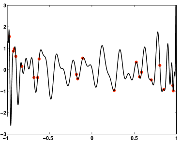
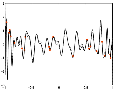
Figure 1: (a) A Legendre-$5$-sparse polynomial of maximal degree $N=80$, and its exact reconstruction from $20$ samples drawn independently from the Chebyshev distribution. (b) The same polynomial (solid line), and its approximate reconstruction from $20$ samples corrupted with noise (dashed line).

To be more complete, we plot a phase diagram illustrating, for $N=300$, and several values of $s/m$ and $m/N$ between $0$ and $.7$, the success rate of $\ell_{1}$-minimization in exactly recovering Legendre $s$-sparse polynomials $g(x)=\sum_{k=0}^{N-1}c_{k}L_{k}(x)$. The results, illustrated in Figure $2$, show a sharp transition between uniform recovery (in black) and no recovery whatsoever (white). This transition curve is similar to the phase transition curves obtained for other compressive sensing matrix ensembles, e.g. the random partial discrete Fourier matrix or the Gaussian ensemble. For more details, we refer the reader to [19].

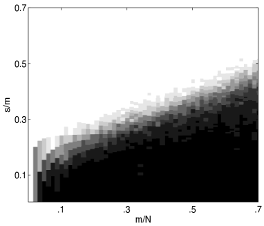
Figure 2: Phase diagram illustrating the transition between uniform recovery (black) and no recovery whatsoever (white) of Legendre-sparse polynomials of sparsity level $s$ and using $m$ measurements, as $s$ and $m$ vary over the range $s\leq m\leq N=300$. In particular, for each pair $(s/m,m/N)$, we record the rate of success out of $50$ trials of $\ell_{1}$-minimization in recovering $s$-sparse coefficient vectors with random support over $[N]$ and with i.i.d. standard Gaussian coefficients from $m$ measurements distributed according to the Chebyshev measure.

4 Sparse recovery via restricted isometry constants

We prove Theorem 2.1 by showing that the preconditioned Legendre matrix ${\cal A}\Phi$ satisfies the restricted isometry property (RIP) [13, 12]. To begin, let us recall the notion of restricted isometry constants for a matrix $\Psi$.

Definition 4.1 (Restricted isometry constants).

Let $\Psi\in{\mathbb{C}}^{m\times N}$. For $s\leq N$, the restricted isometry constant $\delta_{s}$ associated to $\Psi$ is the smallest number $\delta$ for which

$$(1-\delta)\|c\|_{2}^{2}\leq\|\Psi c\|_{2}^{2}\leq(1+\delta)\|c\|_{2}^{2}$$ (8)

for all $s$-sparse vectors $c\in{\mathbb{C}}^{N}$.

Informally, the matrix $\Psi$ is said to have the restricted isometry property if $\delta_{s}$ is small for $s$ reasonably large compared to $m$. For matrices satisfying the restricted isometry property, the following $\ell_{1}$-recovery results can be shown [12, 9, 23, 22].

Theorem 4.2 (Sparse recovery for RIP-matrices).

Let $\Psi\in{\mathbb{C}}^{m\times N}$. Assume that its restricted isometry constant $\delta_{2s}$ satisfies

$$\delta_{2s}<3/(4+\sqrt{6})\approx 0.4652.$$ (9)

Let $x\in{\mathbb{C}}^{N}$ and assume noisy measurements $y=\Psi x+\eta$ are given with $\|\eta\|_{2}\leq\varepsilon$. Let $x^{\#}$ be the minimizer of

$$\arg\min_{z\in{\mathbb{C}}^{N}}\quad\|z\|_{1}\mbox{ subject to }\quad\|\Psi z-y\|_{2}\leq\varepsilon.$$ (10)

Then

$$\|x-x^{\#}\|_{2}\leq C_{1}\frac{\sigma_{s}(x)_{1}}{\sqrt{s}}+C_{2}\varepsilon,$$ (11)

and

$$\|x-x^{\#}\|_{1}\leq D_{1}\sigma_{s}(x)_{1}+D_{2}\sqrt{s}\varepsilon.$$ (12)

The constants $C_{1},D_{1},C_{2},D_{2}>0$ depend only on $\delta_{2s}$. In particular, if $x$ is $s$-sparse then reconstruction is exact, $x^{\#}=x$.

The constant in (9) is the result of several refinements. Candès provided the value $\sqrt{2}-1$ in [9], Foucart and Lai the value $0.45$ in [23], while the version in (9) was shown in [22]. The proof of (11) can be found in [9]. The $\ell_{1}$-error bound (12) is straightforward from these calculations, but does not seem to appear explicitly in the literature.

So far, all good constructions of matrices with the restricted isometry property use randomness. The RIP constant for a matrix whose entries are (properly normalized) independent and identically distributed Gaussian or Bernoulli random variables satisfies $\delta_{s}\leq\delta$ with probability at least $1-e^{-c_{1}(\delta)m}$ provided

$$m\geq c_{2}(\delta)s\log(N/s);$$ (13)

see for example [5, 13, 33, 32]. To be more precise, it can be shown that $c_{1}(\delta)=C_{1}\delta^{2}$ and $c_{2}(\delta)=C_{2}\delta^{-2}$. Lower bounds for Gelfand widths of $\ell_{1}$-balls show that the bound (13) is optimal [20, 15, 24].

If one allows for slightly more measurements than the optimal number (13), the restricted isometry property also holds for a rich class of structured random matrices; the structure of these matrices allows for fast matrix-vector multiplication, which accelerates the speed of reconstruction procedures such as $\ell_{1}$ minimization. A quite general class of structured random matrices are those associated to bounded orthonormal systems. This concept is introduced in [32], although it is already contained somewhat implicitly in [13, 35] for discrete systems. Let ${\cal{D}}$ be a measurable space – for instance, a measurable subset of ${\mathbb{R}}^{d}$ – endowed with a probability measure $\nu$. Further, let $\{\psi_{j}$, $j\in[N]\}$, be an orthonormal system of (real or complex-valued) functions on ${\cal D}$, i.e.,

$$\int_{\cal D}\psi_{j}(x)\overline{\psi_{k}(x)}d\nu(x)=\delta_{j,k},\quad k,j\in[N].$$ (14)

If this orthonormal system is uniformly bounded,

$$\sup_{j\in[N]}\|\psi_{j}\|_{\infty}=\sup_{j\in[N]}\sup_{x\in{\cal D}}|\psi_{j}(x)|\leq K$$ (15)

for some constant $K\geq 1$, we call systems $\{\psi_{j}\}$ satisfying this condition bounded orthonormal systems.

Theorem 4.3 (RIP for bounded orthonormal systems).

Consider the matrix $\Psi\in{\mathbb{C}}^{m\times N}$ with entries

$$\Psi_{\ell,k}=\psi_{k}(x_{\ell}),\quad\ell\in[m],k\in[N],$$ (16)

formed by i.i.d. samples $x_{\ell}$ drawn from the orthogonalization measure $\nu$ associated to the bounded orthonormal system $\{\psi_{j}$, $j\in[N]\}$ having uniform bound $K\geq 1$ in (15). If

$$m\geq C\delta^{-2}K^{2}s\log^{3}(s)\log(N),$$ (17)

then with probability at least $1-N^{-\gamma\log^{3}(s)},$ the restricted isometry constant $\delta_{s}$ of $\frac{1}{\sqrt{m}}\Psi$ satisfies $\delta_{s}\leq\delta$. The constants $C,\gamma>0$ are universal.

We note that condition (17) is stated slightly different in [32], namely as

$$\frac{m}{\log(m)}\geq C\delta^{-2}K^{2}s\log^{2}(s)\log(N).$$

However, it is easily seen that (17) implies this condition (after possibly adjusting constants). Note also that (17) is implied by the simpler condition

$$m\geq CK^{2}\delta^{-2}s\log^{4}(N).$$

An important special case of a bounded orthonormal system is the random partial Fourier matrix, which is formed by choosing a random subset of $m$ rows from the $N\times N$ discrete Fourier matrix. The continuous analog of this system is the matrix associated to the trigonometric polynomial basis $\{x\mapsto e^{2\pi inx},\quad n=0,\ldots,N-1\}$ evaluated at $m$ sample points chosen independently from the uniform measure on $[0,1]$. Note that the trigonometric system has corresponding optimal uniform bound $K=1$. Another example is the matrix associated to the Chebyshev polynomial system evaluated at sample points chosen independently from the corresponding orthogonalization measure, the Chebyshev measure. In this case, $K=\sqrt{2}$.

5 Proof of Theorem 2.1

As a first approach towards recovering Legendre-sparse polynomials from random samples, one may try to apply Theorem 4.3 directly, selecting the sampling points $\{x_{j},j\in[m]\}$, independently from the normalized Lebesgue measure on $[-1,1]$, the orthogonalization measure for the Legendre polynomials. However, as shown in [37], the $L^{\infty}$-norms of the Legendre polynomials grow according to $\|L_{n}\|_{\infty}=|L_{n}(1)|=|L_{n}(-1)|=(2n+1)^{1/2}$. Applying $K=\|L_{N-1}\|_{\infty}=(2N-1)^{1/2}$ in Theorem 4.3 produces a required number of samples

$$m\asymp N\delta^{-2}s\log^{3}(s)\log(N).$$

Of course, this bound is completely useless, because the required number of samples is now larger than $N$ – an almost trivial estimate. Therefore, in order to deduce sparse recovery results for the Legendre polynomials, we must take a different approach.

Despite growing unboundedly with increasing degree at the endpoints $+1$ and $-1$, an important characteristic of the Legendre polynomials is that they are all bounded by the same envelope function. The following result [37, Theorem 7.3.3], gives a precise estimate for this bound.

Lemma 5.1.

For all $n\geq 1$ and for all $x\in[-1,1]$,

$$(1-x^{2})^{1/4}|\thinspace L_{n}(x)\thinspace|<2\pi^{-1/2}\Big{(}1+\frac{1}{2n}\Big{)}^{1/2},\hskip 14.22636pt-1\leq x\leq 1;$$

here, the constant $2\pi^{-1/2}$ cannot be replaced by a smaller one.

Proof of Theorem 2.1.

In light of Lemma 5.1, we apply a preconditioning technique to transform the Legendre polynomial system into a bounded orthonormal system. Consider the functions

$$Q_{n}(x)=(\pi/2)^{1/2}(1-x^{2})^{1/4}L_{n}(x).$$ (18)

The matrix $\Psi$ with entries $\Psi_{j,n}=Q_{n-1}(x_{j})$ may be written as $\Psi={\cal A}\Phi$ where ${\cal A}$ is the diagonal matrix with entries $a_{j,j}=(\pi/2)^{1/2}(1-x_{j}^{2})^{1/4}$ as in Theorem 5.1, and $\Phi\in{\mathbb{R}}^{m\times N}$ is the Legendre matrix with entries $\Phi_{j,n}=L_{n-1}(x_{j})$. By Lemma 5.1, the system $\{Q_{n}\}$ is uniformly bounded on $[-1,1]$ and satisfies the bound $\|Q_{n}\|_{\infty}\leq\sqrt{2+\frac{1}{n}}\leq\sqrt{3}$. Due to the orthonormality of the Legendre system with respect to the normalized Lebesgue measure on $[-1,1]$, the $Q_{n}$ are orthonormal with respect to the Chebyshev probability measure $d\nu(x)=\pi^{-1}(1-x^{2})^{-1/2}dx$ on $[-1,1]$:

$$\int_{-1}^{1}\pi^{-1}Q_{n}(x)Q_{k}(x)(1-x^{2})^{-1/2}dx = \frac{1}{2}\int_{-1}^{1}L_{n}(x)L_{k}(x)dx=\delta_{n,k}.$$

Therefore, the $\{Q_{n}\}$ form a bounded orthonormal system in the sense of Theorem 4.3 with uniform bound $K=\sqrt{3}$. By Theorem 4.3, the renormalized matrix $\frac{1}{\sqrt{m}}\Psi$ has the restricted isometry property with constant $\delta_{s}\leq\delta$ with high probability once $m\geq C\delta^{-2}s\log^{4}(N)$. We then apply Theorem 4.2 to the noisy samples $\frac{1}{\sqrt{m}}{\cal A}y$ where $y=\big{(}g(x_{1})+\eta_{1},...,g(x_{m})+\eta_{m}\big{)}$ and observe that $\|{\cal A}\eta\|_{\infty}\leq\varepsilon$ implies $\frac{1}{\sqrt{m}}\|{\cal A}\eta\|_{2}\leq\varepsilon$. This gives Theorem 2.1.

∎

6 Universality of the Chebyshev measure

The Legendre polynomials are orthonormal with respect to the uniform measure on $[-1,1]$; we may instead consider an arbitrary weight function $v$ on $[-1,1]$, and the polynomials $\{p_{n}\}$ that are orthonormal with respect to $v$. Subject to a mild continuity condition on $v$, a result similar to Lemma 5.1 concerning the uniform growth of ${p_{n}}$ still holds, and the sparse recovery results of Theorem 2.1 extend to this more general scenario. In all cases, the sampling points are chosen according to the Chebyshev measure.

Let us recall the following general bound, see e.g. Theorem 12.1.4 in Szegö [37].

Theorem 6.1.

Let $v$ be a weight function on $[-1,1]$ and set $f_{v}(\theta)=v(\cos\theta)|\sin(\theta)|$. Suppose that $f_{v}$ satisfies the Lipschitz-Dini condition, that is,

$$|f_{v}(\theta+\delta)-f_{v}(\theta)|\leq L|\log(1/\delta)|^{-1-\lambda},\quad\mbox{ for all }\theta\in[0,2\pi),\delta>0,$$ (19)

for some constants $L,\lambda>0$. Let $\{p_{n},n\in{\mathbb{N}}_{0}\}$, be the associated orthonormal polynomial system. Then

$$(1-x^{2})^{1/4}v(x)^{1/2}|p_{n}(x)|\leq C_{v}\quad\mbox{ for all }n\in{\mathbb{N}},x\in[-1,1].$$ (20)

The constant $C_{v}$ depends only on the weight function $v$.

The Lipschitz-Dini condition (19) is satisfied for a range of Jacobi polynomials $p_{n}=p_{n}^{(\alpha,\beta)}$, $n\geq 0,$ $\alpha,\beta\geq-1/2$, which are orthogonal with respect to the weight function $v(x)=(1-x)^{\alpha}(1+x)^{\beta}$. The Legendre polynomials are a special case of the Jacobi polynomials corresponding to $\alpha=\beta=0$; more generally, the case $\alpha=\beta$ correspond to the ultraspherical polynomials. The Chebyshev polynomials are another important special case of ultraspherical polynomials, corresponding to parameters $\alpha=\beta=-1/2$, and Chebyshev measure.

For any orthonormal polynomial system satisfying a bound of the form (20), the following RIP-estimate applies.

Theorem 6.2.

Consider a positive weight function $v$ on $[-1,1]$ satisfying the conditions of Theorem 6.1, and consider the orthonormal polynomial system $\{p_{n}\}$ with respect to the probability measure $d\nu(x)=c\,v(x)dx$ on $[-1,1]$ where $c^{-1}=\int_{-1}^{1}v(x)dx$.

Suppose that $m$ sampling points $(x_{1},\ldots,x_{m})$ are drawn independently at random from the Chebyshev measure, and consider the $m\times N$ composite matrix $\Psi={\cal A}\Phi$, where $\Phi$ is the matrix with entries $\Phi_{j,n}=p_{n-1}(x_{j})$, and ${\cal A}$ is the diagonal matrix with entries $a_{j,j}=(c\pi)^{1/2}(1-x_{j}^{2})^{1/4}v(x_{j})^{1/2}$. Assume that

$$m\geq C\delta^{-2}s\log^{3}(s)\log(N).$$ (21)

Then with probability at least $1-N^{-\gamma\log^{3}(s)}$ the restricted isometry constant of the composite matrix $\frac{1}{\sqrt{m}}\Psi=\frac{1}{\sqrt{m}}{\cal A}\Phi$ satisfies $\delta_{s}\leq\delta$. The constant $C$ depends only on $v$, and the constant $\gamma>0$ is universal.

Proof of Theorem 6.2.

Observe that $\Psi_{j,n}=Q_{n-1}(x_{j})$, where

$$Q_{n}(x)=(c\pi)^{1/2}(1-x^{2})^{1/4}v(x)^{1/2}p_{n}(x).$$

Following Theorem 6.1, the system $\{Q_{n}\}$ is uniformly bounded on $[-1,1]$ and satisfies the bound $\|Q_{n}\|_{\infty}\leq(c\pi)^{-1/2}C_{v}$; moreover, due to the orthonormality of the polynomials $\{p_{n}\}$ with respect to the measure $d\nu(x)$, the $\{Q_{n}\}$ are orthonormal with respect to the Chebyshev measure:

$$\int_{-1}^{1}\pi^{-1}Q_{n}(x)Q_{k}(x)(1-x^{2})^{-1/2}dx = \int_{-1}^{1}cp_{n}(x)p_{k}(x)v(x)dx=\delta_{n,k}.$$ (22)

Therefore, the $\{Q_{n}\}$ form a bounded orthonormal system with associated matrix $\Psi$ as in Theorem 6.2 formed from samples $\{x_{j}\}$ drawn from the Chebyshev distribution. Theorem 4.3 implies that the renormalized composite matrix $\frac{1}{\sqrt{m}}\Psi$ has the restricted isometry property as stated. ∎

Corollary 6.3.

Consider an orthonormal polynomial system $\{p_{n}\}$ associated to a measure $v$ satisfying the conditions of Theorem 6.1. Let $N,m,s\in{\mathbb{N}}$ satisfy the conditions of Theorem 6.2, and consider the matrix $\Psi={\cal{A}}\Phi$ as defined there.

Then with probability exceeding $1-N^{-\gamma\log^{3}(s)}$ the following holds for all polynomials $g(x)=\sum_{k=0}^{N-1}c_{k}p_{k}(x)$. If noisy sample values $y=\big{(}g(x_{1})+\eta_{1},\ldots,g(x_{m})+\eta_{m}\big{)}=\Phi c+\eta$ are observed, and $\|\eta\|_{\infty}\leq\varepsilon$, then the coefficient vector $c=(c_{0},c_{1},\ldots,c_{N-1})$ is recoverable to within a factor of its best $s$-term approximation error and to a factor of the noise level by solving the inequality-constrained $\ell_{1}$-minimization problem

$$c^{\#}=\arg\min_{z\in{\mathbb{R}}^{N}}\|z\|_{1}\quad\mbox{ subject to }\quad\|{\cal A}\Phi z-{\cal A}y\|_{2}\leq\sqrt{m}\varepsilon.$$ (23)

Precisely,

$$\|c-c^{\#}\|_{2}\leq\frac{C_{1}\sigma_{s}(c)_{1}}{\sqrt{s}}+D_{1}\varepsilon,$$

and

$$\|c-c^{\#}\|_{1}\leq C_{2}\sigma_{s}(c)_{1}+D_{2}\sqrt{s}\varepsilon.$$ (24)

The constants $C_{1},C_{2},D_{1},D_{2}$ and $\gamma$ are universal.

As a byproduct of Theorem 6.2, we also obtain condition number estimates for preconditioned orthogonal polynomial matrices that should be of interest on their own, and improve on the results in [26]. Theorem 6.2 implies that all submatrices of a preconditioned random orthogonal polynomial matrix $\frac{1}{\sqrt{m}}\Psi=\frac{1}{\sqrt{m}}{\cal A}\Phi\in{\mathbb{R}}^{m\times N}$ with at most $s$ columns are simultaneously well-conditioned, provided (21) holds. If one is only interested in a particular subset of $s$ columns, i.e., a particular subset of $s$ orthogonal polynomials, the number of measurements in (21) can be reduced to

$$m\geq Cs\log(s);$$ (25)

see Theorem 7.3 in [32] for more details.

Stability with respect to the sampling measure.

The requirement that sampling points $x_{j}$ are drawn from the Chebyshev measure in the previous theorems can be relaxed somewhat. In particular, suppose that the sampling points $x_{j}$ are drawn not from the Chebyshev measure, but from a more general probability measure $d\nu(x)=\rho(x)dx$ on $[-1,1]$ with $\rho(x)\geq c^{\prime}(1-x^{2})^{-1/2}$ (and $\int_{-1}^{1}\rho(x)dx=1$). Now assume a weight function $v$ satisfying the Lipschitz-Dini condition (19) and the associated orthonormal polynomials $p_{n}(x)$ are given. Then, by Theorem 6.1 the functions

$$Q_{n}(x)=(c\pi)^{1/2}\rho(x)^{-1/2}v(x)^{1/2}p_{n}(x)$$ (26)

form a bounded orthonormal system with respect to the probability measure $\tilde{c}\rho(x)v(x)dx$. Therefore, all previous arguments are again applicable. We note, however, that taking $\rho(x)dx$ to be the Chebyshev measure produces the smallest constant $K$ in the boundedness condition (15) due to normalization reasons.

7 Recovery in infinite-dimensional function spaces

We can transform the previous results into approximation results on the level of continuous functions. For simplicity, we restrict the scope of this section to the Legendre basis, although all of our results extend to any orthonormal polynomial system with a Lipschitz-Dini weight function, as well as to the trigonometric system, for which related results have not been worked out yet, either.

We introduce the following weighted norm on continuous functions in $[-1,1]$:

$$\|f\|_{\infty,w}:=\sup_{x\in[-1,1]}|f(x)|w(x),\quad w(x)=\sqrt{\frac{\pi}{2}}(1-x^{2})^{1/4}.$$

Further, we define

$$\sigma_{N,s}(f)_{\infty,w}:=\inf_{c\in{\mathbb{R}}^{N}}\left\{\sigma_{s}(c)_{1}+\sqrt{s}\|f-\sum_{k=0}^{N-1}c_{k}L_{k}\|_{\infty,w}\right\}.$$ (27)

The above quantity involves the best $s$-term approximation error of $c$, as well as the ability of Legendre coefficients $c\in{\mathbb{R}}^{N}$ to approximate the given function $f$ in the $L_{\infty}$-norm. In some sense, it provides a mixed linear and nonlinear approximation error. The $c$ which “balances” both error terms determines $\sigma_{N,s}(f)_{\infty}$. The factor $\sqrt{s}$ scaling the “linear approximation part” may seem to lead to non-optimal estimates at first sight, but later on, the strategy will actually be to choose $N$ in dependence of $s$ such that $\sigma_{N,s}(f)_{\infty}$ becomes of the same order as $\sigma_{s}(c)_{1}$. In any case, we note the (suboptimal) estimate

$$\sigma_{N,s}(f)_{\infty,w}\leq\sqrt{s}\,\rho_{N,s}(f)_{\infty,w},$$

where

$$\rho_{N,s}(f)_{\infty,w}:=\inf_{c\in{\mathbb{R}}^{N},\|c\|_{0}\leq s}\|f-\sum_{k=0}^{N-1}c_{k}L_{k}\|_{\infty,w}.$$

Our aim is to obtain a good approximation to a continuous function $f$ from $m$ sample values, and to compare the approximation error with $\sigma_{N,s}(f)_{\infty,w}$. We have

Proposition 7.1.

Let $N,m,s$ be given with

$$m\geq Cs\log^{3}(s)\log(N).$$

Then there exist sampling points $x_{1},\ldots,x_{m}$ (i.e., chosen i.i.d. from the Chebyshev measure) and an efficient reconstruction procedure (i.e., $\ell_{1}$-minimization), such that for any continuous function $f$ with associated error $\sigma_{N,s}(f)_{\infty,w}$, the polynomial $P$ of degree at most $N$ reconstructed from $f(x_{1}),\ldots,f(x_{m})$ satisfies

$$\|f-P\|_{\infty,w}\leq C^{\prime}\sigma_{N,s}(f)_{\infty,w}.$$

The constants $C,C^{\prime}>0$ are universal.

The quantity $\sigma_{N,s}(f)_{\infty,w}$ involves the two numbers $N$ and $s$. We now describe how $N$ can be chosen in dependence on $s$, reducing the number of parameters to one. We illustrate this strategy below in a more concrete situation. To describe the setup we introduce analogues of the Wiener algebra in the Legendre polynomial setting. Let $c(f)$ with entries

$$c_{k}(f)=\frac{1}{2}\int_{-1}^{1}f(x)L_{k}(x)dx,\quad k\in{\mathbb{N}}_{0},$$

denote the vector of Fourier-Legendre coefficients of $f$. Then we define

$$A_{p}:=\{f\in C[-1,1],\|c(f)\|_{p}<\infty\},\quad 0<p\leq 1,$$

with quasi-norm $\|f\|_{A_{p}}:=\|c(f)\|_{p}$. The use of the $p$-norm is motivated by the Stechkin estimate (1) below, which tells us that elements in $\ell_{p}$ can be considered compressible. Since $\|L_{k}w\|_{\infty}\leq\sqrt{3}$ it follows that

$$f(x)w(x)=\sum_{k\in{\mathbb{N}}_{0}}c_{k}(f)L_{k}(x)w(x)$$

converges uniformly for $f\in A_{1}$, so that $fw\in C[-1,1]$, and $\|f\|_{\infty,w}\leq\sqrt{3}\|f\|_{A_{1}}$. Since $\|f\|_{A_{1}}\leq\|f\|_{A_{p}}$ for $0<p\leq 1$ this holds also for $f\in A_{p}$, $0<p\leq 1$. Now we introduce

$$\sigma_{s}(f)_{A_{1}}:=\inf_{c\in\ell_{2}({\mathbb{N}}_{0}),\|c\|_{0}\leq s}\|f-\sum_{k}c_{k}L_{k}\|_{A_{1}}=\sigma_{s}(c(f))_{1}.$$

By Stechkin’s estimate (1) (which is also valid in infinite dimensions) we have, for $0<q<1$,

$$\sigma_{s}(f)_{A_{1}}\leq s^{1-1/q}\|f\|_{A_{q}}.$$ (28)

Our goal is to realize this approximation rate for $f\in A_{q}$ when only sample values of $f$ are given. Additionally, the number of samples should be close (up to $\log$-factors) to the number $s$ of degrees of freedom of the reconstructed function. Unfortunately, for this task we have to at least know roughly a finite set $[N]$ containing the Fourier-Legendre coefficients of a good $s$-sparse approximation of $f$. In order to deal with this problem, we introduce, for $\alpha>0$, a weighted Wiener type space $A_{1,\alpha}$, containing the functions $f\in C[-1,1]$ with finite norm

$$\|f\|_{A_{1,\alpha}}:=\sum_{k\in{\mathbb{N}}_{0}}(1+k)^{\alpha}|c_{k}(f)|.$$

One should imagine $\alpha\ll 1$ very small, so that $f\in A_{1,\alpha}$ does not impose a severe restriction on $f$, compared to $f\in A_{q}$. Then instead of $f\in A_{q}$ we make the slightly stronger requirement $f\in A_{q}\cap A_{1,\alpha}$, $0<q<1$. The next theorem states that under such assumptions, the optimal rate (28) can be realized when only a small number of sample values of $f$ are available.

Theorem 7.2.

Let $0<q<1$, $\alpha>0$, and $m,s\in{\mathbb{N}}$ be given such that

$$m\geq C\alpha^{-1}\left(\frac{1}{q}-\frac{1}{2}\right)s\log^{4}(s).$$ (29)

Then there exist sampling points $x_{1},\ldots,x_{m}\in[-1,1]$ (i.e., random Chebyshev points) such that for every $f\in A_{q}\cap A_{1,\alpha}$ a polynomial $P$ of degree at most $N=\lceil s^{(1/q-1/2)/\alpha}\rceil$ can be reconstructed from the sample values $f(x_{1}),\ldots,f(x_{m})$ such that

$$\frac{1}{\sqrt{3}}\|f-P\|_{\infty,w}\leq\|f-P\|_{A_{1}}\leq C(\|f\|_{A_{q}}+\|f\|_{A_{1,\alpha}})s^{1-1/q}.$$ (30)

Note that up to $\log$-factors the number of required samples is of the order of the number $s$ of degrees of freedom (the sparsity) allowed in the estimate (1), and the reconstruction error (30) satisfies the same rate. Clearly $\ell_{1}$-minimization or greedy alternatives can be used for reconstruction. This result may be considered as an extension of the theory of compressive sensing to infinite dimensions (although all the key tools are actually finite dimensional).

7.1 Proof of Proposition 7.1

Let $P_{opt}=\sum_{k=0}^{N-1}c_{k,opt}L_{k}$ denote the polynomial of degree at most $N-1$ whose coefficient vector $c_{opt}$ realizes the approximation error $\sigma_{N,s}(f)_{\infty,w}$, as defined in (27). The samples $f(x_{1}),\ldots,f(x_{m})$ can be seen as noise corrupted samples of $P_{opt}$, that is, $f(x_{\ell})=P_{opt}(x_{\ell})+\eta_{\ell},$ and $|\eta_{\ell}|w(x_{\ell})\leq\|f-P_{opt}\|_{\infty,w}:=\varepsilon$. The preconditioned system reads then $f(x_{\ell})w(x_{\ell})=\sum_{k=0}^{N-1}c_{k,opt}L_{k}(x_{\ell})w(x_{\ell})+\varepsilon_{\ell}$, with $|\varepsilon_{\ell}|\leq\varepsilon$. According to Theorem 4.3 and Theorem 5.1, the matrix $\frac{1}{\sqrt{m}}\Psi$ consisting of entries $\Psi_{\ell,k}=w(x_{\ell})L_{k-1}(x_{\ell})$ satisfies the RIP with high probability, provided the stated condition on the minimal number of samples holds. Due to Theorem 4.2, an application of noise-aware $\ell_{1}$-minimization (10) to $y=(f(x_{\ell})w(x_{\ell}))_{\ell=1}^{m}$ with $\varepsilon$ replaced by $\sqrt{m}\varepsilon$ yields a coefficient vector $c$ satisfying $\|c-c_{opt}\|_{1}\leq C_{1}\sigma_{s}(c_{opt})_{1}+C_{2}\sqrt{s}\varepsilon$. We denote the polynomial corresponding to this coefficient vector by $P(x)=\sum_{k=0}^{N-1}c_{k}L_{k}(x)$. Then

$$\|f-P\|_{\infty,w} \leq\|f-P_{opt}\|_{\infty,w}+\|P_{opt}-P\|_{\infty,w}\leq\frac{\sigma_{N,s}(f)_{\infty,w}}{\sqrt{s}}+\sqrt{3}\|c-c_{opt}\|_{1}$$

$$\leq\frac{\sigma_{N,s}(f)_{\infty,w}}{\sqrt{s}}+\sqrt{3}\Big{[}C_{1}\sigma_{s}(c_{opt})_{1}+C_{2}\sqrt{s}\|f-P_{opt}\|_{\infty,w}\Big{]}\leq C\sigma_{N,s}(f)_{\infty,w}.$$

This completes the proof.

The attentive reader may have noticed that our recovery method, noise-aware $\ell_{1}$-minimization (10), requires knowledge of $\sigma_{N,s}(f)$, see also Remark 2.2(c). One may remove this drawback by considering CoSaMP [38] or Iterative Hard Thresholding [7] instead. The required error estimate in $\ell_{1}$ follows from the $\ell_{2}$-stability results for these algorithms in [7, 38], as both algorithms produce a $2s$-sparse vector, see [6, p. 87] for details.

7.2 Proof of Theorem 7.2

Let $f\in A_{q}\cap A_{1,\alpha}$ with Fourier Legendre coefficients $c_{k}(f)$. Let $N>s$ be a number to be chosen later and introduce the truncated Legendre expansion

$$f_{N}(x)=\sum_{k=0}^{N-1}c_{k}(f)L_{k}(x),$$

which has truncated Fourier-Legendre coefficient vector $c^{(N)}$ with entries $c^{(N)}_{k}=c_{k}(f)$ if $k<N$ and $c^{(N)}_{k}=0$ otherwise. Clearly, $\|c^{(N)}\|_{q}\leq\|c(f)\|_{q}=\|f\|_{A_{q}}.$ Further note that

$$\frac{1}{\sqrt{3}}\|f-f_{N}\|_{\infty,w} \leq\|f-f_{N}\|_{A_{1}}=\|c-c^{(N)}\|_{1}=\sum_{k=N}^{\infty}|c_{k}(f)|\leq N^{-\alpha}\sum_{k=N}^{\infty}(1+k)^{\alpha}|c_{k}(f)|$$

$$\leq N^{-\alpha}\|f\|_{A_{1,\alpha}}.$$

Now we proceed similarly as in the proof of Theorem 7.1 and treat the samples of $f$ as perturbed samples of $f_{N}$, that is $f_{N}(x_{j})=f(x_{j})+\eta_{j}$ with $|\eta_{j}|w(x_{j})\leq\|f-f_{N}\|_{\infty,w}\leq\sqrt{3}N^{-\alpha}\|f\|_{A_{1,\alpha}}$. Then following the same arguments as in the proof of Theorem 7.1, if

$$m\geq Cs\log^{3}(s)\log(N),$$ (31)

we can reconstruct a coefficient vector $\widetilde{c}$ from samples $f(x_{1}),\ldots,f(x_{m})$ with support contained in $\{0,1,\ldots,N-1\}$ such that

$$\|c^{(N)}-\widetilde{c}\|_{1}\leq C_{1}\sigma_{s}(c^{(N)})_{1}+C_{2}\sqrt{s}\|f-f_{N}\|_{\infty,w}\leq C_{1}s^{1-1/q}\|f\|_{A_{q}}+C_{2}\sqrt{s}N^{-\alpha}\|f\|_{A_{1,\alpha}}.$$

Here, we applied Stechkin’s estimate (1). Therefore,

$$\|c-\widetilde{c}\|_{1} \leq\|c-c^{(N)}\|_{1}+\|c^{(N)}-\widetilde{c}\|_{1}\leq N^{-\alpha}\|f\|_{A_{1,\alpha}}+C_{1}s^{1-1/q}\|f\|_{A_{q}}+C_{2}\sqrt{s}N^{-\alpha}\|f\|_{A_{1,\alpha}}$$

$$\leq C_{1}s^{1-1/q}\|f\|_{A_{q}}+C_{2}^{\prime}\sqrt{s}N^{-\alpha}\|f\|_{A_{1,\alpha}}.$$

Now we choose

$$N=\lceil s^{1/\alpha(1/q-1/2)}\rceil$$ (32)

which yields $\sqrt{s}N^{-\alpha}\leq s^{1-1/q}$. With this choice

$$\frac{1}{\sqrt{3}}\|f-\tilde{f}_{N}\|_{\infty,w}\leq\|f-\tilde{f}_{N}\|_{A_{1}}=\|c-\widetilde{c}\|_{1}\leq C^{\prime}(\|f\|_{A_{q}}+\|f\|_{A_{1,\alpha}})s^{1-1/q}.$$

Plugging (32) into (31) yields (29), and the proof is finished.

Remark 7.3.

Analogous function approximation results can be derived from Theorem 6.2 for any orthogonal polynomial basis whose weight function satisfies the conditions of Theorem 6.1. The associated norm is $\|f\|_{v,\infty}=\|\sqrt{3}v^{1/2}fw\|_{\infty}.$ For the Chebyshev polynomials, $\|f\|_{v,\infty}=\|f\|_{\infty}$, and the corresponding function approximation results in this case are with respect to the unweighted uniform norm.

Acknowledgments

The authors would like to thank Albert Cohen, Simon Foucart, and Joseph Ward for valuable discussions on this topic, and are also grateful to Laurent Gosse for helpful comments. Rachel Ward gratefully awknowledges the partial support of National Science Foundation Postdoctoral Research Fellowship. Holger Rauhut gratefully acknowledges support by the Hausdorff Center for Mathematics and by the WWTF project SPORTS (MA 07-004). Parts of this manuscript have been written during a stay of the first author at the Laboratoire Jacques-Louis Lions of Université Pierre et Marie Curie in Paris. He greatly acknowledges the warm hospitality of the institute and especially of his host Albert Cohen.

References

- [1] P. Abrial, Y. Moudden, J. Starck, J. Fadili, J. Delabrouille, and M. Nguyen. CMB data analysis and sparsity. Stat. Methodol., 5:289–298, 2008.
- [2] B. Alexeev and R. Ward. On the complexity of Mumford-Shah type regularization, viewed as a relaxed sparsity constraint. IEEE Trans. Image Process., 2010. To appear.
- [3] D. Alireza and O. Houman. A non-adapted sparse approximation of PDEs with stochastic inputs. J. Comp. Physics, 230(8):3015–3034, 2011.
- [4] G. Andrews, R. Askey, and R. Roy. Special functions. Cambridge University Press, 1999.
- [5] R. G. Baraniuk, M. Davenport, R. A. DeVore, and M. Wakin. A simple proof of the restricted isometry property for random matrices. Constr. Approx., 28(3):253–263, 2008.
- [6] R. Berinde. Advances in sparse signal recovery methods. Masters Thesis., 2009.
- [7] T. Blumensath and M. Davies. Iterative hard thresholding for compressed sensing. Appl. Comput. Harmon. Anal., 27(3):265–274, 2009.
- [8] L. Brutman. Lebesgue functions for polynomial interpolation—a survey. Ann. Numer. Math., 4(1-4):111–127, 1997.
- [9] E. J. Candès. The restricted isometry property and its implications for compressed sensing. C. R. Acad. Sci. Paris S’er. I Math., 346:589–592, 2008.
- [10] E. J. Candès, J., T. Tao, and J. Romberg. Robust uncertainty principles: exact signal reconstruction from highly incomplete frequency information. IEEE Trans. Inform. Theory, 52(2):489–509, 2006.
- [11] E. J. Candès and J. Romberg. Sparsity and incoherence in compressive sampling. Inverse Problems, 23(3):969–985, 2007.
- [12] E. J. Candès, J. Romberg, and T. Tao. Stable signal recovery from incomplete and inaccurate measurements. Comm. Pure Appl. Math., 59(8):1207–1223, 2006.
- [13] E. J. Candès and T. Tao. Near optimal signal recovery from random projections: universal encoding strategies? IEEE Trans. Inform. Theory, 52(12):5406–5425, 2006.
- [14] S. S. Chen, D. L. Donoho, and M. A. Saunders. Atomic decomposition by Basis Pursuit. SIAM J. Sci. Comput., 20(1):33–61, 1999.
- [15] A. Cohen, W. Dahmen, and R. A. DeVore. Compressed sensing and best k-term approximation. J. Amer. Math. Soc., 22(1):211–231, 2009.
- [16] A. Cohen, R. DeVore, and C. Schwab. Analytic regularity and polynomial approximation of parametric and stochastic elliptic PDEs. Anal. Appl., 2011. to appear.
- [17] P. Daniel. Fast algorithms for discrete polynomial transforms on arbitrary grids. Linear Algebra and its Applications, 366:353 – 370, 2003.
- [18] G. Davis, S. Mallat, and M. Avellaneda. Adaptive greedy approximations. Constr. Approx., 13(1):57–98, 1997.
- [19] D. Donoho and J. Tanner. Observed universality of phase transitions in high-dimensional geometry, with implications for modern data analysis and signal processing. Philosophical Transactions of the Royal Society, 367(1906):4273–4293, 2009.
- [20] D. L. Donoho. Compressed sensing. IEEE Trans. Inform. Theory, 52(4):1289–1306, 2006.
- [21] M. Fornasier and H. Rauhut. Compressive Sensing. In O. Scherzer, editor, Handbook of Mathematical Methods in Imaging, pages 187–228. Springer, 2011.
- [22] S. Foucart. A note on guaranteed sparse recovery via -minimization. Appl. Comput. Harmon. Anal., 29(1):97–103, 2010.
- [23] S. Foucart and M. Lai. Sparsest solutions of underdetermined linear systems via -minimization for . Appl. Comput. Harmon. Anal., 26(3):395–407, 2009.
- [24] S. Foucart, A. Pajor, H. Rauhut, and T. Ullrich. The Gelfand widths of -balls for . J. Complexity, 26(6):629–640, 2010.
- [25] A. C. Gilbert and J. A. Tropp. Signal recovery from random measurements via orthogonal matching pursuit. IEEE Trans. Inform. Theory, 53(12):4655–4666, 2007.
- [26] K. Gröchenig, B. Pötscher, and H. Rauhut. Learning trigonometric polynomials from random samples and exponential inequalities for eigenvalues of random matrices. preprint, 2007.
- [27] D. Healy Jr., D. Rockmore, P. Kostelec, and S. Sean. FFTs for the 2-Sphere - Improvements and Variations. J. Fourier Anal. Appl., 9:341–385, 1996.
- [28] R. James, M. Dennis, and N. Daniel. Fast discrete polynomial transforms with applications to data analysis for distance transitive graphs. SIAM J. Comput., 26(4):1066–1099, 1997.
- [29] D. Potts, G. Steidl, and M. Tasche. Fast algorithms for discrete polynomial transforms. Math. Comp., 67:1577–1590, 1998.
- [30] H. Rauhut. Random sampling of sparse trigonometric polynomials. Appl. Comput. Harmon. Anal., 22(1):16–42, 2007.
- [31] H. Rauhut. On the impossibility of uniform sparse reconstruction using greedy methods. Sampl. Theory Signal Image Process., 7(2):197–215, 2008.
- [32] H. Rauhut. Compressive Sensing and Structured Random Matrices. In M. Fornasier, editor, Theoretical Foundations and Numerical Methods for Sparse Recovery, volume 9 of Radon Series Comp. Appl. Math., pages 1–92. deGruyter, 2010.
- [33] H. Rauhut, K. Schnass, and P. Vandergheynst. Compressed sensing and redundant dictionaries. IEEE Trans. Inform. Theory, 54(5):2210 – 2219, 2008.
- [34] H. Rauhut and R. Ward. Sparse recovery for spherical harmonic expansions. In Proc. SampTA, Singapore, 2011.
- [35] M. Rudelson and R. Vershynin. On sparse reconstruction from Fourier and Gaussian measurements. Comm. Pure Appl. Math., 61:1025–1045, 2008.
- [36] K. Schnass and P. Vandergheynst. Dictionary preconditioning for greedy algorithms. IEEE Trans. Signal Process., 56(5):1994–2002, 2008.
- [37] G. Szegö. Orthogonal Polynomials. American Mathematical Society, Providence, RI, 1975.
- [38] J. Tropp and D. Needell. CoSaMP: Iterative signal recovery from incomplete and inaccurate samples. Appl. Comput. Harmon. Anal., 26(3):301–321, 2008.
- [39] M. Tygert. Fast algorithms for spherical harmonic expansions, II. J. Comput. Phys., 227(8):4260–4279, 2008.