Diffractive Microlensing III: Astrometric Signatures

Abstract

Gravitational lensing is generally treated in the geometric optics limit; however, when the wavelength of the radiation approaches or exceeds the Schwarzschild radius of the lens, diffraction becomes important. Although the magnification generated by diffractive gravitational lensing is well understood, the astrometric signatures of diffractive microlensing are first derived in this paper along with a simple closed-form bound for the astrometric shift. This simple bound yields the maximal shifts for substellar lenses in solar neighbourhood observed at 20 GHz, accessible to high sensitivity, high angular resolution radio telescopes such as the proposed Square Kilometre Array (SKA).

1 Introduction

Gravitational microlensing is a powerful tool to probe the constituents of the solar neighbourhood, the Galaxy and beyond (e.g. Wambsganss, 2006). In particular Gaudi & Bloom (2005) have propose astrometric microlensing as a technique to detect sub-stellar objects in the solar neighbourhood, and Heyl (2010a, b) argued that diffraction could provide important constraints on lensing objects in the Kuiper belt and beyond. The combination of diffraction and astrometric lensing offers a new dimension to microlensing surveys.

Several authors have examined gravitational lensing including the effects of diffraction (e.g. Ingel & Rubakha, 1978; Elster, 1980; Bontz & Haugan, 1981; Deguchi & Watson, 1986; Ulmer & Goodman, 1995; Takahashi, 2004). However, the focus has almost entirely been on the magnification of the image. An exception is the work of Labeyrie (1994) that examines the possibility of using a planetary mass lens as a telescope. This letter will examine the astrometry of diffractive lensing; that is how does lensing affect the centroid of the light distribution including the effects of diffraction. As diffraction can amplify the magnification of a gravitational lens, so too does it increase the motion of the image. Measuring the motion of the image can provide constraints on the lens, source and their relative motion.

The commissioning of the Square Kilometre Array (SKA) over the next decade will offer an unprecedented view of the radio sky. Koopmans & de Bruyn (2000) outlines some prospects for using the SKA to understand strongly lensed quasars and especially the small-scale structure of the lensing object. This letter also examines primarily the lensing of quasars but focuses on nearby lensing objects with the hopes to provide constraints on the number of small bodies in the solar neighbourhood. Such constraints are difficult to obtain otherwise. The letter is divided into a calculation (§ 2) of the astrometric signature of lensing both in the diffractive and geometric optics regimes, a description of the results (§ 3) and an evaluation of the prospects of observing this effect (§ 4).

2 Calculations

Schneider et al. (1992) give the magnification for a point source including diffraction

$$\mu_{\omega}=\left|I\right|^{2}=\left|\int_{u_{d}}^{\infty}u^{1-if}e^{iu^{2}/2}J_{0}(uv)du\right|^{2}.$$ (1)

where $u$ is the radial coordinate that integrates over the plane of the lens, $J_{0}$ is the Bessel function of the first kind, and $v$ is the impact parameter of the source relative to the lens. Both $u$ and $v$ are dimensionless and measure lengths in units of the reduced Fresnel length,

$$l_{\hbox{\rm\scriptsize Fr}}=\sqrt{\frac{c}{\omega_{d}}\frac{D_{d}D_{ds}}{D_{s}}}$$ (2)

where $\omega_{d}=\omega(1+z_{d})$ is the angular frequency of the radiation as it passes the lens. Hence the value of $u_{d}$ which compares the angular size ($r_{d}/D_{d}$) of the occulting portion of the lens to angular scale of its diffraction pattern ($\lambda/r_{d}$) is given by

$$u_{d}=r_{d}\sqrt{\frac{\omega_{d}}{c}\frac{D_{s}}{D_{d}D_{ds}}}=\frac{r_{d}}{l_{\hbox{\rm\scriptsize Fr}}}.$$ (3)

The parameter $f$ is given by

$$f=\frac{\omega_{d}}{c}\frac{D_{s}}{D_{d}D_{ds}}R_{E}^{2}$$ (4)

where $D_{s}$ is the distance to the source, $D_{d}$ is the distance to the lens, $D_{ds}$ is the distance between the source and the lens, $z_{d}$ is the redshift of the lens, and the Einstein radius is the characteristic length of the lens,

$$R_{E}=\sqrt{2R_{S}\frac{D_{d}D_{ds}}{D_{s}}}=\sqrt{f}l_{\hbox{\rm\scriptsize Fr}}$$ (5)

for the Schwarzschild lens where $R_{S}=2GM_{d}/c^{2}$ where $G$ is Newton’s gravitational constant, $M_{d}$ is the mass of the lens and $c$ is the speed of light; therefore, the value of

$$f=2R_{S}\frac{\omega_{d}}{c}.$$ (6)

The parameter $f$ compares the wavelength of the radiation to the Schwarzschild radius of the lens. The limit where the gravitational field of the lens is negligible is $f=0$, so the effect of gravity on the form of the integral, Eq. (1), is quite modest. In a cosmological context all of the distances given are angular diameter distances.

Here the occultation will be neglected (i.e. $u_{d}\rightarrow 0$). The integral can be calculated in closed form in terms of the confluent hypergeometric function (${}_{1}F_{1}(a;b;z)$) for $u_{d}=0$. Gradshteyn & Ryzhik (1994) give relation (6.631.1) which in this particular case yields

$$\int_{0}^{\infty}u^{1-if}e^{iu^{2}/2}J_{0}(uv)du\!\! = \!\!e^{\pi f/4}e^{i\left(\pi-f\ln 2\right)/2}\Gamma\left(1-i\frac{f}{2}\right)\times$$ (7)

$$~{}{}_{1}F_{1}\left(1-i\frac{f}{2};1;-i\frac{v^{2}}{2}\right).$$

The result for $f=0$ is simply $i\exp(-iv^{2}/2)$.

2.1 Astrometry

The gradient of the phase of the incoming radiation points to the apparent location of an unresolved source on the sky. This location on the image plane is given by

$${\bar{u}}=-\Im\frac{\partial\ln I}{\partial v}=\Im\left[\frac{1}{I}\int_{u_{d}}^{\infty}u^{2-if}e^{iu^{2}/2}J_{1}(uv)du\right].$$ (8)

where $\Im$ denotes the imaginary part of the expression it precedes. The first equality will also hold for an asymmetric lens where $\langle\vec{u}\rangle=-\Im\nabla\ln V$. If $u_{d}=0$ the following expression holds

$${\bar{u}}=v\Re\left[\left(1-i\frac{f}{2}\right)\frac{{}_{1}F_{1}\left(2-i\frac{f}{2};2;-i\frac{v^{2}}{2}\right)}{{}_{1}F_{1}\left(1-i\frac{f}{2};1;-i\frac{v^{2}}{2}\right)}\right]$$ (9)

where for $f=0$ the quantity in the brackets is unity and $\Re$ denotes the real part of the expression in brackets.

For values of $f,v\ll 1$ the ratio of the hypergeometric functions can be conveniently approximated by Gauss’s continued fraction (Cuyt et al., 2008)

$$\frac{{}_{1}F_{1}\left(a+1;b+1;z\right)}{{}_{1}F_{1}\left(a;b;z\right)}=\displaystyle\frac{1}{1-\displaystyle\frac{{\displaystyle\frac{b-a}{b(b+1)}z}}{1+\displaystyle\frac{{\displaystyle\frac{a+1}{(b+1)(b+2)}z}}{1-\displaystyle\frac{{\displaystyle\frac{b-a+1}{(b+2)(b+3)}z}}{1+\displaystyle\frac{{\displaystyle\frac{a+2}{(b+3)(b+4)}z}}{1-\ddots}}}}}.$$ (10)

Although several techniques exist to determine the range of the confluent hypergeometric function (e.g. Karp & Sitnik, 2009), it is simpler in this case to resort to numerical experimentation, it appears that the follow inequality obtains

$$0\leq v\left({\bar{u}}-v\right)\leq 2f$$ (11)

with the value oscillating between the two extremes. This yields useful estimates for the magnitude of the astrometric shift from diffractive lensing. Furthermore, the value in the brackets of Eq. 9 is purely real at these extrema, so they are also extrema of the magnification.

2.2 Physical Optics

For values of $f,v\gg\ 1$ the value given by Eq. (8) may be estimated by using a physical optics approximation. In particular the square root of Eq. (1) may be approximated up to a constant phase by (Schneider et al., 1992)

$$I\approx e^{i\phi_{+}}\sqrt{\mu_{+}}+e^{i(\phi_{-}-\pi/2)}\sqrt{\mu_{-}}$$ (12)

where

$$u_{\pm}=\frac{1}{2}\left(v\pm\sqrt{v^{2}+4f}\right),$$ (13)

$$\phi_{\pm}=\frac{u_{\pm}^{2}}{2}-f\ln|u_{\pm}|-u_{\pm}v$$ (14)

and

$$\mu_{\pm}=\frac{u_{\pm}}{v}\left|\frac{du_{\pm}}{dv}\right|=\frac{1}{2}\left(\frac{v^{2}+2f}{v\sqrt{v^{2}+4f}}\pm 1\right).$$ (15)

The values $u_{\pm}$ are defined to be positive and negative while $\mu_{\pm}$ is always positive. The two images have opposite parity. It is natural to interpret this as a negative value of the magnification for one of the images; hence there is an additional $\pi/2$ of geometric phase of the positive term relative to the negative term. This choice may seem rather arbitrary, but it results from the stationary phase approximation of Eq. (1) where one extremum ($u_{-}$) is a saddle point. This allows a simple expression like Eq. (12) to approximate the results of Eq. (1) accurately for large values of $f$. For more complicated lens geometries, the phase lag is proportional to the Morse index of the image (Schneider et al., 1992).

Furthermore, essentially by design the following holds $d\phi_{\pm}/dv=-u_{\pm}$. Combining these results with Eq. (8) yields an estimate for

$${\bar{u}} \approx \frac{1}{\mu}\Bigg{\{}\mu_{+}u_{+}+\mu_{-}u_{-}+$$

$$~{}~{}~{}\left(\mu_{+}\mu_{-}\right)^{1/2}\bigg{[}\left(u_{+}+u_{-}\right)\cos\Delta\phi$$

$$~{}~{}~{}+\frac{1}{2}\left(\frac{d\ln\mu_{+}}{dv}-\frac{d\ln\mu_{+}}{dv}\right)\sin\Delta\phi\bigg{]}\Bigg{\}}$$

where at this level of approximation the total magnification is

$$\mu\approx\frac{v^{2}+2f\left(1+\cos\Delta\phi\right)}{v\sqrt{v^{2}+4f}}$$ (17)

and

$$\Delta\phi=\phi_{+}-\phi_{-}+\frac{\pi}{2}~{}\mathrm{and}~{}\mu_{+}\mu_{-}=\frac{f^{2}}{v^{2}\left(v^{2}+4f\right)}.$$ (18)

The various definitions allow some further simplifications yielding

$${\bar{u}}\approx\frac{1}{\mu}\left[\frac{v^{2}+f\left(3+\cos\Delta\phi\right)}{\sqrt{v^{2}+4f}}+\frac{2f\sin\Delta\phi}{v\left(v^{2}+4f\right)}\right].$$ (19)

The result from geometric optics obtains by neglecting the terms with $\Delta\phi$ yielding,

$${\bar{u}}\approx\frac{v\left(v^{2}+3f\right)}{v^{2}+2f}.$$ (20)

The maximum displacement due to lensing in the geometric limit is $8^{-1/2}R_{E}$ at $v=2^{1/2}R_{E}$.

3 Results

Diffractive effects can have a dramatic effect on the trajectory of images of gravitationally lensed sources. In particular from Fig 1 is it apparent that the maximal displacement is much larger when diffractive effects are considered. As in the geometric limit, the centroid lies along the line connecting the centre of the lens and the source. Furthermore, the centroid lies further from the centre of the lens than the source. The observed oscillations point back to the location of the lens, so the detection of three oscillations combined with the presumably known proper motion of the source determines the impact parameter between the source and lens, the proper motion, mass and distance of the lens unequivocally.

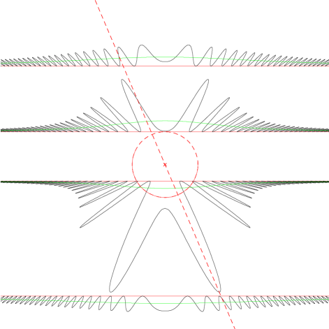
Figure 1: The figure depicts the paths of images and sources for various impact parameters with the angular position of the lens fixed. The dashed circle denotes the Einstein radius of the lens. The red line gives the path of the source (unlensed). The green curve gives the path of the image without diffractive effects. The black curve gives the path of the image with diffraction for ($f=10$). The impact parameters from top to bottom are $3R_{E},R_{E},0.5R_{E}$ and $4R_{E}$. The dashed red line indicates how to translate a location along the path of the source to the location of the image centroid.

Fig. 2 shows that the displacement of the image centroid from the source location oscillates between no displacement and $2R_{E}^{2}/v$ outward. Furthermore, the minimal displacement occurs at a maxima in the magnification. The maxima of $v\left({\bar{u}}-v\right)$ (where the black curves touch the blue curve) occur at a minima of the magnification. In particular because for small values of $v$ and large values of $f$ the magnification is well approximated by a Bessel function (Schneider et al., 1992), it is straightforward to estimate the peak displacement that occurs near the first zero of the Bessel function $J_{0}(x)$ at $x\approx 2.4$ to be

$$\left({\bar{u}}-v\right)_{\mathrm{max}}\approx 0.83fR_{E}~{}\mathrm{at}~{}\frac{v}{R_{E}}\approx 2.4f^{-1}~{}\mathrm{for}~{}f\gg\ 1.$$ (21)

For smaller values of $f$, the peak displacement occurs for smaller values of $v$ than given by this formula, and therefore the displacement is larger than given here. In particular, the displacement is larger than the geometric limit (Eq. 20) for $f>0.17$. The maxima for $f=0.17$ occurs at $v/R_{E}\approx 5.5$ as opposed to 14 as estimated from Eq. (21).

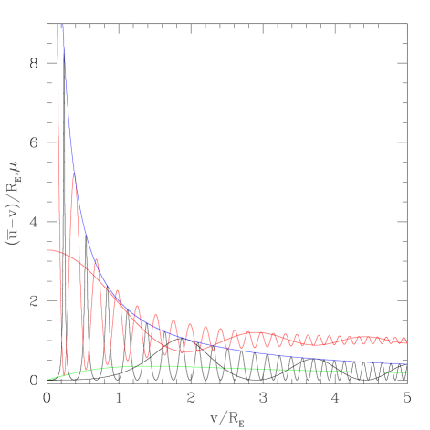
Figure 2: The total magnification (red) and the difference (black) between the apparent radial position of the image centroid and the location of the source as a function of source location relative to the centre of the lens. The green curve gives the displacement according to geometric optics. The rapid oscillations are for $f=10$ as in Fig. 1, and the slower oscillations are for $f=1$. The blue curve gives the envelope of $2R_{E}^{2}/v.$

The envelope of the displacement, $2R_{E}^{2}/v$, is robust regardless of the value of $f$ or $v$, so it is natural to focus on the displacement by dividing by the size of the envelope, yielding Fig. 3. The approximation from physical optics is depicted by the dashed curve and follows the accurate calculation for $f=10$ very closely. However, for $f=1$ the agreement is much poorer. Furthermore, the physical optics approximation does not precisely follow the simple envelope as the deviations below zero and above two manifest. Even if one is more careful and approximates the magnification as a Bessel function, the envelope only obtains approximately. The presence of the strict envelope results from an apparently thus-far unknown property of the hypergeometric functions and allows useful approximation of the possible signal.

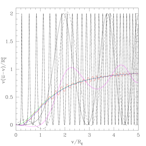
Figure 3: The difference between the apparent radial position of the image centroid and the location of the source as a function of source location relative to the centre of the lens. The result for $f=1$ is the slowly varying sinusoidal curve and $f=10$ is the more rapidly varying one. The dashed curves give the results using the physical optics approximation from Eq. (19). For $f=10$ it is nearly indistinguishable from complete result. The displacement from geometric optics is plotted in green. Notice for $f=10$ there are about three peaks over a length of one Einstein radius for small values of $v$ and more for larger values. The other colours assume that the angular radius of the source equals the Einstein radius. Blue is the geometric optics result, red is for $f=10$ and magenta is $f=1$.

Fig. 3 also shows the effect of a finite source size to wash out the observed oscillations toward the geometric optics result. It is not surprising that the rapid oscillations suffer a greater decrement than for $f=1$. However, observational realities push the use of higher frequency observations to get finer angular resolution. For a fixed source size and impact parameter, the size of the oscillations is proportional to $f^{-3/2}$ while the angular resolution of a given telescope is proportional to frequency, increasing with $f$. Consequently if angular resolution is the only factor in the accuracy of determining the centroid, the signal-to-noise of the measurement of the centroid is proportional to $f^{-1/2}$; it makes more sense to perform the measurement at lower frequency. On the other hand with increased flux, the centroid can be determined more accurately, so this conclusion could change depending on the spectrum of the object.

Determining the centroid of an object’s emission is generally more difficult than measuring the flux itself; therefore, searching for the diffractive flux variation would generally be more fruitful than looking for an astrometric signature, unless the flux from the source is inherently noisy making the oscillation in the magnification difficult to detect. Heyl (2010b) outlines using quasars as powerful tools to detect diffractive microlensing. Flat spectrum radio quasars generally have high brightness temperatures, so large fluxes from small solid angles. This can dramatically increase the expected signal-to-noise ratio for a diffractive microlensing event. On the other hand the flux from the quasar may be inherently noisy dominating the detector noise upon which Heyl (2010b) focus. For such objects the astrometric signature of diffractive microlensing is a powerful tool.

Because of the envelope of the oscillation, it is straightforward to estimate the magnitude of the displacement oscillation given the impact parameter of the source relative to the lens ($b$) and the properties of the lens itself. In particular for a planetary mass lens the following obtains

$$\left({\bar{u}}-v\right)_{\mathrm{max}}\approx 0.5\frac{M_{d}}{\mathrm{M}_{\oplus}}\left(\frac{D_{d}}{1~{}\mathrm{pc}}\right)^{-1}\!\!\!\!\left(\frac{b}{0.1~{}\mathrm{mas}}\right)^{-1}\!\!\!\!\mathrm{mas}$$ (22)

as along as the source may be considered compact compared to the diffraction fringes. In particular the SKA is expected to have an angular resolution of about 5 mas at 20 GHz, or $f\approx 7$ for an Earth-mass lens (Schilizzi et al., 2007). Whether or not SKA measurements could constrain the positions of quasars to less than a milliarcsecond remains to be seen, but the VLBA typically measures the positions of sources about 10 microarcseconds, so the SKA could in principle achieve 60 microseconds with its larger minimum wavelength and smaller size, detecting Earth-mass lenses out to about 10 pc with a source impact parameter of 0.1 milliarcseconds. If one were especially lucky and found an especially close encounter between the lens and source, the maximal displacement is

$$\left({\bar{u}}-v\right)_{\mathrm{max}}\approx 1\left(\frac{M_{d}}{\mathrm{M}_{\oplus}}\right)^{3/2}\!\!\!\left(\frac{D_{d}}{1~{}\mathrm{pc}}\right)^{-1/2}\!\!\!\!\!\frac{\nu}{20~{}\mathrm{GHz}}\mathrm{mas}$$ (23)

in principle detectable with the SKA out to 250 pc. However, at such a distance the lens subtends such a small angle that finite-source effects are likely to be important.

Heyl (2010b) calculated the expected event rate of substellar objects lensing bulge stars in the OGLE-II catalogue that can also be detected with the Square Kilometre Array (about 80,000 stars) under the assumption that the density of substellar objects in the disk of our Galaxy is about one-tenth of the total density. The total optical depth of such lenses is about $2\times 10^{-9}$. The calculation neglected the possibility of substellar objects in the Galactic halo and assumed that a lensing event lasts one day. Under these assumptions, the event rate where a source and lens align to within one Einstein radius is about once per 14 years. The lensing of bulge stars could yield an astrometric signature of diffractive microlensing in addition to the magnification signature discussed in Heyl (2010b).

This event rate can be scaled to the microlensing rate for flat spectrum radio quasars for which the astrometric signature may be easier to measure. To achieve a rate of once per decade about 100,000 radio sources would have to be monitored. Because one expects the lenses to be restricted to the plane of the Galaxy more or less, only those quasars that lie within ten degrees of the Galactic equator should be considered as sources (about two steradians). The number counts of flat-spectrum radio quasars give the expected event rate as a function of the quasar radio flux. de Zotti et al. (2010) compile the number of counts of radio-loud quasars at several frequencies. In particular above several GHz the sample will be dominated by flat-spectrum sources; furthermore, this is where the SKA is sensitive. From the number counts at 8.4 GHz (Windhorst et al., 1993; Fomalont et al., 2002; Henkel & Partridge, 2005) one can estimate that there are about $10^{5}$ flat-spectrum radio sources within ten degrees of the Galactic plane with fluxes greater than 4 mJy. To get a sample of $10^{6}$ sources requires a flux limit of 0.3 mJy. What remains to be seen is how well future instruments will be able to centroid such sources as a function of flux. These limits of course refer to the flux of the entire source not just the high brightness temperature components that will show the most dramatic astrometric signatures.

4 Conclusions

The continuous monitoring of compact, distant radio sources may provide new way to probe the constituents of our solar neighbourhood, in particular freely, floating sub-stellar objects. The astrometric signatures of diffractive microlensing can provide an estimate of the mass, distance and proper motion of the lensing object, possibly allowing follow-up observations of the lens itself. Astrometric lensing even without diffraction effects can provide this information as well (Wambsganss, 2006); however, diffraction typically amplifies the astrometric signature and radio observations often offer much higher angular resolution on the order of ten milliarcseconds versus several hundred milliarcseconds in the optical.

This letter has used the specifications of the SKA as a benchmark. Clearly the high angular resolution and high frequency offered by the SKA are helpful for the detection of astrometric lensing in the radio; however, the high sensitivity of the SKA may not strictly be necessary if one focuses on bright radio sources. Perhaps, a purpose-built very-large baseline array of phased dipoles could achieve the needed angular resolution (and possibly even a finer resolution than the SKA) with a sufficient sensitivity to continuously determine the centroids the brightest radio sources to the needed accuracy to detect low-mass objects in the solar neighbourhood. Furthermore, such a monitoring campaign could yield new insights on quasar physics as well as other ancillary results. The low expected optical depth for these events of about $2\times 10^{-9}$ would required the monitoring of 100,000 radio sources to achieve even the modest event rate of once per decade. These sources could be quasars or bulge giants, although the effect should be more pronounced with the high brightness-temperture quasars.

References

- Bontz & Haugan (1981) Bontz R. J., Haugan M. P., 1981, Astrophys. Sp. Sci., 78, 199
- Cuyt et al. (2008) Cuyt A., Petersen V. B., Verdonk B., Waadeland H., Jones W. B., 2008, Handbook of Continued Fractions for Special Functions. Springer, Berlin, p. 319
- de Zotti et al. (2010) de Zotti G., Massardi M., Negrello M., Wall J., 2010, Astron. Astrophys. Rev. , 18, 1
- Deguchi & Watson (1986) Deguchi S., Watson W. D., 1986, Astrophys. J, 307, 30
- Elster (1980) Elster T., 1980, Astrophys. Sp. Sci., 71, 171
- Fomalont et al. (2002) Fomalont E. B., Kellermann K. I., Partridge R. B., Windhorst R. A., Richards E. A., 2002, Astron. J, 123, 2402
- Gaudi & Bloom (2005) Gaudi B. S., Bloom J. S., 2005, Astrophys. J, 635, 711
- Gradshteyn & Ryzhik (1994) Gradshteyn I. S., Ryzhik I. M., 1994, Table of Integrals, Series, and Products, fifth edn. Academic Press
- Henkel & Partridge (2005) Henkel B., Partridge R. B., 2005, Astrophys. J, 635, 950
- Heyl (2010a) Heyl J., 2010a, Monthly Notices, 402, L39
- Heyl (2010b) Heyl J., 2010b, Monthly Notices, submitted
- Ingel & Rubakha (1978) Ingel L. K., Rubakha N. R., 1978, Radiofizika, 21, 87
- Karp & Sitnik (2009) Karp D., Sitnik S. M., 2009, J. Approx. Theory, 161, 337
- Koopmans & de Bruyn (2000) Koopmans L. V. E., de Bruyn A. G., 2000, in M. P. van Haarlem ed., Perspectives on Radio Astronomy: Science with Large Antenna Arrays Micro and Strong Lensing with the Square Kilometer Array: the Mass-Function of Compact Objects in High-Redshift Galaxies. pp 213–+
- Labeyrie (1994) Labeyrie A., 1994, Astronomy and Astrophysics, 284, 689
- Schilizzi et al. (2007) Schilizzi R. T., et al., 2007, Technical report, Preliminary Specifications for the Square Kilometre Array. Square Kilometre Array
- Schneider et al. (1992) Schneider P., Ehlers J., Falco E. E., 1992, Gravitational Lenses. Springer, Berlin
- Takahashi (2004) Takahashi R., 2004, Astron. Astrophys., 423, 787
- Ulmer & Goodman (1995) Ulmer A., Goodman J., 1995, Astrophys. J, 442, 67
- Wambsganss (2006) Wambsganss J., 2006, Gravitational Lensing: Strong, Weak and Micro. Springer, Berlin
- Windhorst et al. (1993) Windhorst R. A., Fomalont E. B., Partridge R. B., Lowenthal J. D., 1993, Astrophys. J, 405, 498