Another Look at Climate Sensitivity

Zusammenfassung

We revisit a recent claim that the Earth’s climate system is characterized by sensitive dependence to parameters; in particular, that the system exhibits an asymmetric, large-amplitude response to normally distributed feedback forcing. Such a response would imply irreducible uncertainty in climate change predictions and thus have notable implications for climate science and climate-related policy making. We show that equilibrium climate sensitivity in all generality does not support such an intrinsic indeterminacy; the latter appears only in essentially linear systems. The main flaw in the analysis that led to this claim is inappropriate linearization of an intrinsically nonlinear model; there is no room for physical interpretations or policy conclusions based on this mathematical error. Sensitive dependence nonetheless does exist in the climate system, as well as in climate models — albeit in a very different sense from the one claimed in the linear work under scrutiny — and we illustrate it using a classical energy balance model (EBM) with nonlinear feedbacks. EBMs exhibit two saddle-node bifurcations, more recently called “tipping points,”which give rise to three distinct steady-state climates, two of which are stable. Such bistable behavior is, furthermore, supported by results from more realistic, nonequilibrium climate models. In a truly nonlinear setting, indeterminacy in the size of the response is observed only in the vicinity of tipping points. We show, in fact, that small disturbances cannot result in a large-amplitude response, unless the system is at or near such a point. We discuss briefly how the distance to the bifurcation may be related to the strength of Earth’s ice-albedo feedback.

Keywords: Climate sensitivity, energy balance models, global warming, stability analysis, bifurcations

1 Introduction and motivation

1.1 Climate sensitivity and its implications

Systems with feedbacks are an efficient mathematical tool for modeling a wide range of natural phenomena; Earth’s climate is one of the most prominent examples. Stability and sensitivity of feedback models is, accordingly, a traditional topic of theoretical climate studies (Cess, 1976; Ghil, 1976; Crafoord and Källén, 1978; Schlesinger, 1985, 1986; Cess et al., 1989). Roe and Baker (2007) (RB07 hereafter) have recently advocated existence of intrinsically large sensitivities in an equilibrium model with multiple feedbacks. Specifically, they argued that a small, normally distributed feedback may lead to large-magnitude, asymmetrically distributed values of the system’s response.

Such a property, if valid, would have serious implications for climate dynamics (Allen and Frame, 2007) and for modeling of complex systems in general (Watkins and Freeman, 2008). In this paper, we revisit the dynamical behavior of a general, equilibrium climate model with genuinely nonlinear feedbacks, and focus subsequently on a simple energy-balance model (EBM). We notice that the main, technical part of RB07’s argument is well-known in the climate literature, cf. Schlesinger (1985, 1986), and thus it seems useful to review the associated assumptions and possible interpretations of this result.

We rederive below in Section 1.2 the key equation of RB07 and comment on their purportedly nonlinear analysis in Section 1.3. We then proceed in Section 2 with a more self-consistent version of sensitivity analysis for a nonlinear model. This analysis is applied in Section 3 to a zero-dimensional EBM. Concluding remarks follow in Section 4.

1.2 Roe and Baker’s (2007) linear analysis

We follow here RB07 and assume the following general setup. Let the net radiation $R$ at the top of the atmosphere be related to the corresponding average temperature $T$ at the Earth’s surface by $R=R(T)$. Assume, furthermore, that there exists a feedback $\alpha=\alpha(T)$, which is affected by the temperature change and which can, in turn, affect the radiative balance. Hence, one can write $R=R\left(T,\alpha(T)\right)$.

To study how a small change $\Delta\,R$ in the radiation is related to the corresponding temperature change $\Delta\,T$, one can use the Taylor expansion (Arfken, 1985) to obtain, as $\Delta\,T$ tends to zero,

$$\Delta\,R=\frac{\partial\,R}{\partial\,T}\Delta\,T+\frac{\partial\,R}{\partial\,\alpha}\frac{\partial\,\alpha}{\partial\,T}\Delta\,T+\mathcal{O}\left((\Delta\,T)^{2}\right).$$ (1)

Here, $\mathcal{O}(x)$ is a function such that $\mathcal{O}(x)\leq C\,x$ as soon as $0<x<\epsilon$ for some positive constants $C$ and $\epsilon$.

Introducing the notations

$$\frac{1}{\lambda_{0}}=\frac{\partial\,R}{\partial\,T},\leavevmode\nobreak\ {\rm and\leavevmode\nobreak\ }f=-\lambda_{0}\,\frac{\partial\,R}{\partial\,\alpha}\frac{\partial\,\alpha}{\partial\,T},$$

for the “reference sensitivity” $\lambda_{0}$ and the “feedback factor” $f$, we obtain

$$\Delta\,R=\frac{1-f}{\lambda_{0}}\,\Delta\,T+\mathcal{O}\left((\Delta\,T)^{2}\right),$$ (2)

which readily leads to

$$\Delta\,T=\frac{\lambda_{0}}{1-f}\Delta\,R+\mathcal{O}\left((\Delta\,T)^{2}\right),$$ (3)

as long as $f\neq 1$.

RB07 drop the higher-order terms in (3) to obtain

$$\Delta\,T=\frac{\lambda_{0}}{1-f}\Delta\,R,$$ (4)

which is their equation (S4). This equation leads directly to their main conclusion, namely that a normally distributed feedback factor $f$ results in an asymmetric system response $\Delta\,T$ to a fixed forcing $\Delta\,R$. The purported sensitivity is due to the divergence of the right-hand side (rhs) of Eq. (4) [their equation (S4)] as $f$ approaches unity. Figure 1, which is analogous to Fig. 1 of RB07, illustrates this effect.

Roughly speaking, RB07 use the following argument: If the derivative of $R(T)$ with respect to $T$ is close to 0, then the derivative of $T$ with respect to $R$ is very large, and a small change in the radiation $R$ corresponds to a large change in the temperature $T$. Such an argument, though, is only valid for an essentially linear dependence $R\propto T$. Our straightforward analysis in Section 2 below shows that the sensitivity effect of Fig. 1 is absent in climate models in which genuinely nonlinear feedbacks $R=R(T,\alpha(T))$ are present.

It is worth noticing that, since one seeks the temperature change $\Delta\,T$ that results from a change $\Delta\,R$ in the forcing, it might be preferable to consider the inverse function $T=T(R)$ or, more precisely, $T=T(R,\alpha(R))$ and the corresponding Taylor expansion

$$\Delta\,T=\frac{\partial\,T}{\partial\,R}\Delta\,R+\frac{\partial\,T}{\partial\,\alpha}\frac{\partial\,\alpha}{\partial\,R}\Delta\,R+\mathcal{O}\left((\Delta\,R)^{2}\right).$$

The main conclusions of our analysis will not be affected by the particular choice of direct or inverse expansion, provided the nonlinearities are correctly taken into account.

1.3 Roe and Baker’s “nonlinearänalysis

In this section we address the analysis carried out by RB07 in the supplemental on-line materials, pp. 4-5, Section “Nonlinear feedbacks.” The main conclusion of that analysis was that, given realistic parameter values for the climate system, the effects of possible nonlinearities in the behavior of the function $R=R(T)$ are negligible and do not affect the system’s sensitivity. We point out here two serious flaws in their mathematical reasoning that, each separately and the two together, invalidate such a conclusion.

First, and most importantly, despite their section’s title, the analysis carried out by RB07 is still linear. Indeed, the Taylor expansion in their Eq. (S7) is given by

$$\Delta\,R\approx R^{\prime}\Delta\,T+\frac{1}{2}\,R^{\prime\prime}\,\Delta\,T^{2},$$ (5)

where $(\cdot)^{\prime}$ stands for differentiation with respect to $T$. But RB07 immediately invert this equation for $\Delta\,T$ subject to the assumption

$$\Delta\,T^{2}=\Delta\,T\,\Delta\,T_{0},$$

where $\Delta\,T_{0}$ is a constant. Hence, instead of solving the quadratic Eq. (5), Roe and Baker solve the following linear approximation:

$$\Delta\,R=(R^{\prime}+\frac{1}{2}\,R^{\prime\prime}\,\Delta\,T_{0})\Delta\,T,$$

and thus obtain the key formula [their Eq. (S8)]

$$\Delta\,T\approx\frac{-\lambda_{0}\,\Delta\,R}{1-f-\frac{1}{2}\lambda_{0}\,R^{\prime\prime}\,\Delta\,T_{0}};$$ (6)

the last step uses the, correct, fact that $R^{\prime}=(1-f)/\lambda_{0}$. This equation artificially introduces a divergence point for the temperature at $f=1-(\lambda_{0}/2)\,R^{\prime\prime}\Delta\,T_{0}$, which clearly cannot exist in a quadratic equation. Equation (6) is thus a very crude approximation that significantly deviates from the true solution to the full quadratic equation (5) — which we discuss below in Section 2 — and thus cannot be used to justify general statements about climate models.

The second flaw in the Roe and Baker (2007) reasoning is that, using the model and parameter values they suggest, one readily finds that:

• $R^{\prime}=-2$, i.e., global temperature and radiation are negatively correlated, which is hardly the case for the current climate [e.g., Held and Soden (2000)]. We notice that the negative sign of the correlation follows directly from their Eq. (S10) and is not affected by particular values of the model parameters. Furthermore,

• $R^{\prime\prime}=-0.03$, which means that the model they consider is, indeed, essentially linear, and thus not very realistic.

Although, in this part of their analysis, Roe and Baker assumed that $f=0.4$, it is easy to check that, for all $f<0.95$, their model satisfies $|R^{\prime\prime}/R^{\prime}|<0.1$ and is therewith very close to being linear. To conclude, the effects on nonlinearities are indeed negligible in the particular model studied in this part of the RB07 paper, since the model is very close to being linear; one cannot extrapolate, therefore, their conclusions to climate models with significant nonlinearities.

We next proceed with a mathematically correct sensitivity analysis of a general climate model in the presence of truly nonlinear feedbacks.

2 A self-consistent sensitivity analysis

It is easily seen from the discussion in Section 1.2, especially from Eq. (2), that the relationship (4) is a crude approximation: it is valid only subject to the assumptions that ($a$) the higher-order terms in the expansion of $\Delta\,T$ are vanishingly small:

$$\mathcal{O}\left((\Delta\,T)^{2}\right)\ll\frac{1-f}{\lambda_{0}}\Delta\,T;$$

and ($b$) the quantity in the rhs of this inequality is itself nonzero.

If one assumes, for instance, that $\mathcal{O}\left((\Delta\,T)^{2}\right)\sim C\,(\Delta\,T)^{2}$, where the precise meaning of $g(x)\sim\,f(x)$ is given by $\lim_{x\to 0}g(x)/f(x)=1$, then the assumptions (a,b) above hold for $\Delta\,T$ that satisfy both of the following conditions

$$0<\Delta\,T\ll(1-f)/(\lambda_{0}\,C)\quad{\rm and}\quad 0<\Delta\,T<\epsilon,$$ (7)

where $C$ and $\epsilon$ are defined after Eq. (1). The first of these conditions implies that the range of temperatures within which the approximation (4) works vanishes as the feedback factor $f$ approaches unity. Hence, all the results based on this approximation — including precisely the main conclusions of RB07 — no longer apply outside a vanishingly small neighborhood of $f=1.0$.

The asymptotic behavior we assumed above for $\mathcal{O}\left((\Delta\,T)^{2}\right)$ is not exotic. Consider for instance the function $R=T^{2}$ in the neighborhood of $R=0$. Its Taylor expansion

$$\Delta\,R=2\,T\Delta\,T+\mathcal{O}\left((\Delta\,T)^{2}\right)\,$$

can be used to obtain, ignoring the second-order term,

$$\Delta\,T\approx\Delta\,R/(2\,T).\$$ (8)

The last equation would seem to imply that the growth of $\Delta\,T$ is inversely proportional to $T$ itself, so the change in $T$ should increase infinitely fast as $T$ goes to 0, a rather annoying contradiction.

The way out of this conundrum is to realize that the change $\Delta\,T$ given by Eq. (8) is only valid in a small vicinity of $T=0$ and cannot be extrapolated to larger values. Of course, we all know that the function $R=T^{2}$ is nicely bounded and smooth in the vicinity of 0, but it is essential to take into account the second term in its Taylor expansion in this vicinity to obtain correct results. We show in Section 3 below that this simple example depicts the essential dependence of the Earth surface temperature on the global solar radiative input, for conditions close to those of the current Earth system.

In summary, the linear approximation of the function $R(T)$ derived by RB07 from its Taylor expansion is not valid when $f$ approaches unity. In this case — which is precisely the situation emphasized by these authors — the higher-order terms “hiddenïnside $\mathcal{O}\left((\Delta\,T)^{2}\right)$, which they neglected, are indispensable for a correct, self-consistent climate sensitivity analysis.

A correct analysis of the case when $f$ approaches unity needs to start with a Taylor expansion that keeps the second-order term

$$\Delta\,R=\frac{1-f}{\lambda_{0}}\Delta\,T+a\,(\Delta\,T)^{2}+\mathcal{O}\left((\Delta\,T)^{3}\right),$$

where $a=R^{\prime\prime}/2$. If $\mathcal{O}\left((\Delta\,T)^{3}\right)$ is much smaller than the other two terms on the rhs, then the temperature change can be approximated by a solution of the quadratic equation

$$\frac{1-f}{\lambda_{0}}\Delta\,T+a\,(\Delta\,T)^{2}=\Delta\,R.$$ (9)

The real-valued solutions to the latter equation, if they exist, are given by

$$\Delta\,T_{1,2}=\frac{1}{2}\left(\frac{f-1}{a\,\lambda_{0}}\pm\sqrt{\left(\frac{1-f}{a\,\lambda_{0}}\right)^{2}+\frac{4\,\Delta\,R}{a}}\right).$$

In particular, when $f$ is close to 1.0, then

$$\Delta\,T_{1,2}\approx\pm\sqrt{\frac{\Delta\,R}{a}}.$$ (10)

One can see from Eq. (10) that the proximity of the feedback factor $f$ to unity no longer plays an important role in the qualitative behavior of the equilibrium temperature. This point is further illustrated in Fig. 2 that shows the climate system’s response $\Delta T$ as a function of the feedback factor $f$ for different values of the nonlinearity parameter $a$. The most important observation is that the climate response does not diverge at $f=1$; moreover, the asymmetry of the response due to the changes in feedback factor $f$ rapidly vanishes as soon as the dependence of $\Delta\,R$ on $\Delta\,T$ becomes nonlinear.

In general, one can consider an arbitrary number of terms in the Taylor expansion of $R(T)$. The very fact that one relies on the validity of the Taylor expansion implies that $R(T)$ is bounded and sufficiently smooth; in other words, a divergence of the equilibrium temperature due to a small change in the forcing contradicts the very assumptions on which RB07 based their sensitivity analysis.

3 Sensitivity for energy balance models (EBMs)

We consider here a classical climate model with nonlinear feedbacks to illustrate that, in such a model: (i) the type of sensitivity claimed by RB07 does not exist; and (ii) sensitive dependence may exist, in a very different sense, namely in the neighborhood of bifurcation points, as explained below.

3.1 Model formulation

We consider here a highly idealized type of model that connects the Earth’s temperature field to the solar radiative flux. The key idea on which these models are built is due to Budyko (1969) and Sellers (1969). They have been subsequently generalized and used for many studies of climate stability and sensitivity; see Held and Suarez (1974); North (1975) and Ghil (1976), among others.

The interest and usefulness of these “toymodels resides in two complementary features: (i) their simplicity, which allows a complete and thorough understanding of the key mechanisms involved; and (ii) the fact that their conclusions have been extensively confirmed by studies using much more detailed and presumably realistic models, including general circulation models (GCMs); see, for instance, the reviews of North et al. (1981) and Ghil and Childress (1987).

The main assumption of EBMs is that the rate of change of the global average temperature $T$ is determined only by the net balance between the absorbed radiation $R_{\rm i}$ and emitted radiation $R_{\rm o}$:

$$c\frac{\mathrm{d}T}{\mathrm{d}t}=R_{\rm i}(T)-R_{\rm o}(T).$$ (11)

For simplicity, we follow here the zero-dimensional (0-D) EBM version of Crafoord and Källén (1978) and Ghil and Childress (1987), in which only global, coordinate-independent quantities enter; thus

$$R_{\rm i}=\mu\,Q_{0}\left(1-\alpha(T)\right),\quad R_{\rm o}=\sigma\,g(T)\,T\,^{4}.$$ (12)

In the present formulation, the planetary ice-albedo feedback $\alpha$ decreases in an approximately linear fashion with $T$, within an intermediate range of temperatures, and is nearly constant for large and small $T$. Here $Q_{0}$ is the reference value of the global mean solar radiative input, $\sigma$ is the Stefan-Boltzmann constant, and $g(T)$ is the grayness of the Earth, i.e. its deviation from black-body radiation $\sigma\,T^{4}$. The parameter $\mu\approx 1.0$ multiplying $Q_{0}$ indicates by how much the global insolation deviates from its reference value.

We model the ice-albedo feedback by

$$\alpha(T;\kappa)=c_{1}+c_{2}\,\frac{1-\tanh\left(\kappa\left(T-T_{\rm c}\right)\right)}{2}.$$ (13)

This parametrization represents a smooth interpolation between the piecewise-linear formula of Sellers-type models, like those of Ghil (1976) or Crafoord and Källén (1978), and the piecewise-constant formula of Budyko-type models, like those of Held and Suarez (1974) or North (1975).

Figure 3a shows four profiles of our ice-albedo feedback $\alpha(T)=\alpha(T)$ as a function of $T$, depending on the value of the steepness parameter $\kappa$. The profile for $\kappa\gg 1$ would correspond roughly to a Budyko-type model, in which the albedo $\alpha$ takes only two constant values, high and low, depending on whether $T<T_{\rm c}$ or $T>T_{\rm c}$. The other profiles shown in the figure for smaller values of $\kappa$, correspond to Sellers-type models, in which there exists a transition ramp between the high and low albedo values. Figure 3b shows the corresponding shapes of the radiative input $R_{\rm i}=R_{\rm i}(T)$.

The greenhouse effect is parametrized, as in Crafoord and Källén (1978) and Ghil and Childress (1987), by letting

$$g(T)=1-m\,\tanh\left((T/T_{0})^{6}\right).$$ (14)

Substituting this greenhouse effect parametrization and the one for the albedo into Eq. (11) leads to the following EBM:

$$c\,\dot{T}= \mu \,Q_{0}\left(1-\alpha(T)\right)$$ (15)

$$- \sigma\,T\,^{4}\left[1-m\,\tanh\left((T/T_{0})^{6}\right)\right],$$

where $\dot{T}=\mathrm{d}T/\mathrm{d}t$ denotes the derivative of global temperature $T$ with respect to time $t$.

It is important to note that current concern, both scientific and public, is mostly with the greenhouse effect, rather than with actual changes in insolation. But in a simple EBM model — whether globally averaged, like in Crafoord and Källén (1978) and here, or coordinate-dependent, as in Budyko (1969); Sellers (1969); Held and Suarez (1974); North (1975) or Ghil (1976) — increasing $\mu$ always results in a net increase in the radiation balance. It is thus convenient, and quite sufficient for the purpose at hand, to vary $\mu$ in the incoming radiation $R_{\rm i}$, rather than some other parameter in the outgoing radiation $R_{\rm o}$. We shall return to this point in Section 4.

3.2 Model parameters

The value $S$ of the solar constant, which is the value of the solar flux normally incident at the top of the atmosphere along a straight line connecting the Earth and the Sun, is assumed here to be $S=1370$ Wm^-1. The reference value of the global mean solar radiative input is $Q_{0}=S/4=342.5$, with the factor 1/4 due to Earth’s sphericity.

The parameterization of the ice-albedo feedback in Eq. (13) assumes $T_{c}=273$ K and $c_{1}=0.15$, $c_{2}=0.7$, which ensures that $\alpha(T)$ is bounded between 0.15 and 0.85, as in Ghil (1976); see Fig. 3a. The greenhouse effect parametrization in Eq. (14) uses $m=0.4$, which corresponds to 40% cloud cover, and $T_{0}^{-6}=1.9\times 10^{-15}$ K^-6 (Sellers, 1969; Ghil, 1976). The Stefan-Boltzmann constant is $\sigma\approx 5.6697\times 10^{-8}$Wm^-2K^-4.

3.3 Sensitivity and bifurcation analysis

3.3.1 Two types of sensitivity analysis

We distinguish here between two types of sensitivity analysis for the 0-D EBM (11). In the first type, we assume that the system is driven out of an equilibrium state $T=T_{0}$, for which $R_{\rm i}(T_{0})-R_{\rm o}(T_{0})=0$, by an external force, and want to see whether and how it will return to a new equilibrium state, which may be different from the original one. This analysis refers to the “fast” dynamics of the system, and assumes that $R_{\rm i}(T)-R_{\rm o}(T)\neq 0$ for $T\neq T_{0}$; it is often referred to as linear stability analysis, since it considers mainly small displacements from equilibrium at $t=0$, $T(0)=T_{0}+\theta(0)$, where $\theta(0)$ is of order $\epsilon$, with $0<\epsilon\ll 1$, as defined in Section 2.

The second type of analysis refers to the system’s “slow” dynamics. We are interested in how the system evolves along a branch of equilibrium solutions as the external force changes sufficiently slowly for the system to track an equilibrium state; hence, this second type of analysis always assumes that the solution is in equilibrium with the forcing: $R_{\rm i}(T)-R_{\rm o}(T)=0$ for all $T$ of interest. Typically, we want to know how sensitive model solutions are to such a slow change in a given parameter, and so this type of analysis is called sensitivity analysis. In the problem at hand, we will study — again following Crafoord and Källén (1978) and Ghil and Childress (1987) — how changes in $\mu$, and hence in the global insolation, affect the model’s equilibria.

A remarkable property of the EBM governed by Eq. (11) is the existence of several stationary solutions that describe equilibrium climates of the Earth (Ghil and Childress, 1987). The existence and linear stability of these solutions result from a straightforward bifurcation analysis of the 0-D EBM (11), as well as of its one-dimensional, latutude-dependent counterparts (Ghil, 1976, 1994): there are two linearly stable solutions — one that corresponds to the present climate and one that corresponds to a much colder, “snowball Earth” (Hoffman et al., 1998) — separated by an unstable one, which lies about 10 K below the present climate.

The existence of the three equilibria — two stable and one unstable — has been confirmed by such results being obtained by several distinct EBMs, of either Budyko- or Sellers-type (North et al., 1981; Ghil, 1994). Nonlinear stability, to large perturbations in the initial state, has been investigated by introducing a variational principle for the latitude-dependent EBMs of Sellers (Ghil, 1976) and of Budyko (North et al., 1981) type, and it confirms the linear stability results.

3.3.2 Sensitivity analysis for a 0-D EBM

We analyze here the stability of the “slow,” quasi-adiabatic (in the statistical-physics sense) dynamics of model (15). The energy-balance condition for steady-state solutions $R_{\rm i}=R_{\rm o}$ takes the form

$$\mu\,Q_{0}\left(1-\alpha(T)\right)=\sigma\,T\,^{4}\left[1-m\,\tanh\left((T/T_{0})^{6}\right)\right].$$ (16)

We assume here, following the previously cited EBM work, that the main bifurcation parameter is $\mu$; this happens to agree with the emphasis of Roe and Baker (2007) on climate sensitivity as the dependence of mean temperature $T$ on global solar radiative input, denoted here by $Q=\mu Q_{0}$.

Figure 4 shows the absorbed and emitted radiative fluxes, $R_{\rm i}$ and $R_{\rm o}$, as functions of temperature $T$ for $\mu=0.5,1$ and 2.0. One can see that Eq. (16) may have one or three solutions depending on the value of $\mu$: only the present, relatively warm climate for $\mu=2.0$, only the “deep-freezeclimate for $\mu=0.5$, and all three, including the intermediate, unstable one for present-day insolation values, $\mu=1.0$. These steady-state climate values are shown as a function of the insolation parameter $\mu$ in the bifurcation diagram of Fig. 5.

The “fast” stability analysis (not presented here) shows that small deviations $\theta(0)$ from an equilibrium solution, while all parameter values are kept fixed, may result in two types of dynamics, depending on the initial equilibrium $T_{0}$: fast increase or fast decrease of the initial deviation (Ghil and Childress, 1987). The fast increase characterizes unstable equilibria: a small deviation $\theta(0)$ from such an equilibrium $T_{0}$ forces the solution to go further and further away from the equilibrium. In practice, such equilibria will not be observed, since there are always small, random perturbations of the climate present in the system: just think of weather as representing such perturbations.

The fast decrease of the initial deviation $\theta(0)$ characterizes stable solutions; only such equilibria can be observed in practice. The two stable solution branches of (15) are shown by solid lines in Fig. 5, while the unstable branch is shown by the dashed line. The arrows show the direction in which the temperature will change when drawn away from an equilibrium by external forces. This change, whether away from or towards the nearest equilibrium, is fast compared to the one that occurs along either solution branch (Ghil, 1976, 1994).

3.3.3 Bifurcation analysis

Given the choice of model parameters, the present climate state corresponds to the upper stable solution of Eq. (15), at $\mu=1$ (see Fig. 5). It lies quite close to the bifurcation point $(\mu,T)\approx(0.9,280\leavevmode\nobreak\ {\rm K})$, where the stable and unstable solutions merge.

The so-called normal form of this bifurcation is given by the equation

$$\dot{X}=\bar{\mu}-X^{2},$$ (17)

where $X$ is a suitably normalized form of $T$, and $\bar{\mu}$ is a normalized form of $\mu$. Equation (17) describes the dependence between $T$ and $\mu$ in a small neighborhood of the bifurcation point. In particular, the stable equilibrium branch is described by

$$X=+\sqrt{\bar{\mu}};$$

this result has exactly the same form as the positive solution of Eq. (10), given by our self-consistent analysis of climate sensitivity in the presence of genuine nonlinearities, cf. Section 2. Hence, the derivative ${\rm d}X/{\rm d}{\bar{\mu}}$, and thus ${\rm d}T/{\rm d}\mu$, goes to infinity as the model approaches the bifurcation point; this is exactly the situation discussed earlier in Section 2.

It is important to realize that the parabolic form of temperature dependence on insolation change is not an accident due to the particularly simple form of EBMs. Wetherald and Manabe (1975) clearly showed, in a slightly simplified GCM, that not only the mass-weighted temperature of their total atmosphere, but also the area-weighted temperatures of each of their five model levels, exhibits such a parabolic dependence on fractional radiative input; see Fig. 5 in their paper. Moreover, these authors emphasize that “As stated in the Introduction, it is not, however, reasonable to conclude that the present results are more reliable than the results from the one-dimensional studies mentioned above simply because our model treats the effect of transport explicitly rather than by parameterization. […] Nevertheless, it seems to be significant that both the one-dimensional and three-dimensional models yield qualitatively similar results in many respects.”

In fact, rigorous mathematical results demonstrate that the saddle-node bifurcation whose normal form is given by Eq. (17) occurs in several systems of nonlinear partial differential equations, such as the Navier-Stokes equations (Constantin et al., 1989; Temam, 1997), and not only in ordinary differential equations, like Eqs. (11) and (15) above. We emphasize, though, that this does not cause the temperature to increase rapidly due to small changes in insolation: the presence of the bifurcation point will result in small, positive changes of global temperature for slow, positive changes in $\mu$, while it may throw the climate system into the deep-freeze state for slow, negative changes in $\mu$.

4 Discussion

4.1 How sensitive is climate?

Making projections of climate change for the next decades and centuries, evaluating the human influence on future Earth temperatures, and making normative decisions about current and future anthropogenic impacts on climate are enormous tasks that require solid scientific expertise, as well as responsible moral reasoning. Well-founded approaches to handle the moral aspects of the problem are still being debated [e.g., Hillerbrand and Ghil (2008)]. It is that much more important to master existing tools for acquiring accurate and reliable scientific evidence from the available data and models. Several of these tools come from the realm of nonlinear and complex dynamical systems (Lorenz, 1963; Smale, 1967; Ruelle and Takens, 1971; Ghil and Childress, 1987; Ghil, 1994; Ghil et al., 2008).

A straightforward analysis, carried out in Section 2 of this paper, shows that a proper treatment of the higher-order terms in a climate model with nonlinear feedbacks does not reveal the exaggerated sensitivity to forcing that was used in RB07 to advocate intrinsic unpredictability of climate projections. We emphasize that the error in Roe and Baker’s analysis is not related to their choice of model formulation or of the model parameters nor to their interpretation of model results. The problem is purely a matter of elementary calculus, and is due to inappropriate, and unnecessary, linearization of a nonlinear model.

Our analysis complements, reinforces and goes beyond that of Hannart et al. (2009), who also showed that the claim of RB07 “results from a mathematical artifact.”We notice simply that Hannart and colleagues did not even question the linear approximation framework of RB07 and still concluded that the claims of irreducibility of the spread in the envelope of climate sensitivity are not supported by the RB07 analysis.

To summarize, while the general human concern about climate sensitivity expressed by RB07 should be reasonably shared by many, their scientific conclusions do not follow from their model and its results, when correctly analyzed, as done here in Section 2. Nor are these conclusions supported by other models of greater detail and realism, when properly investigated. Accordingly, conclusions about the likelihood of extreme warming resulting from small changes in anthropogenic forcing can hardly be used to support political proposals [e.g., Allen and Frame (2007)] that claim to provide future directions for the climate-related sciences.

Still, this paper’s analysis does not preclude in any sense the Earth’s temperature from rising significantly in coming years. The methods illustrated here can only be used to study climate sensitivity in the vicinity of a given state; they cannot be applied to investigate climate evolution over tens of years, for example in response to large increases in greenhouse gases or to other major changes in the forcing, whether natural or anthropogenic. This latter problem requires global interdisciplinary efforts and, in particular, the analysis of the entire hierarchy of climate models (Schneider and Dickinson, 1974), from conceptual to intermediate to fully coupled GCMs (Ghil and Robertson, 2000). It also requires a much more careful study of random effects than has been done heretofore (Ghil et al., 2008).

It seems to us that Roe and Baker’s title question ”Why Is Climate Sensitivity So Unpredictable?ßtill remains open.

4.2 Where are the “tipping points”?

The S-shaped diagram of Fig. 5 — see also Fig. 10.6 in Ghil and Childress (1987) and Fig. 4 in Ghil (1994) — was used here to show the smoothness and boundedness of temperature changes as a function of insolation changes, away from a saddle-node bifurcation, like that of Eq. (10) in Section 2 or of Eq. (17) in Section  3.3.3.

This S-shaped curve nevertheless reveals the existence of sensitive dependence of Earth’s temperature on insolation changes, or on other changes in Earth’s net radiation budget, such as may be caused by increasing levels of greenhouse gases, on the one hand, or of aerosols, on the other. This sensitive dependence is quite different from the one advocated by RB07. Namely, if the parameter $\mu$ were to slightly decrease — rather than increase, as it seems to have done since the mid-1970s, in the sense described in the last paragraph of Section 3.1 — then the climate system would be pushed past the bifurcation point at $\mu\approx 0.9$. The only way for the global temperature to go would be down, all the way to a deep-freeze Earth, with much lower temperatures than those of recent, Quaternary ice ages.

It has become common in recent discourse about potentially irreversible climate change to talk about “tipping points”; e.g., Lenton et al. (2008). The term was originally introduced into the social sciences by Gladwell (2000) to denote a point at which a previously rare phenomenon becomes dramatically more common. In the physical sciences, it has been identified with a shift from one stable equilibrium to another one, i.e., to a saddle-node bifurcation, as seen in Fig. 5 here and explained in Section 3.3.3 above.

In the EBM context of Fig. 5, it would require an enormous, almost twofold increase in the insolation in order for a deep-freeze–type equilibrium to reach the bifurcation point at $\mu\approx 1.85$ and jump from there to $T\approx 350$ K, a temperature that sounds equally unpleasant. Within the broader context of the recent debates on how to exit a snowball-Earth state, very large, and possibly implausible increases in ${\rm CO}_{2}$ levels would be required (Pierrehumbert, 2004).

Indeed, the likelihood to actually reach the tipping point to the left of the current climate in Fig. 5 seems to be quite small. Mechanisms for entering a snowball-Earth climate have been recently studied with a number of fairly realistic climate models (Hyde et al., 2000; Donnadieu et al., 2004; Poulsen and Jacob, 2004). Both modeling and independent geological evidence suggest that Earth’s climate can sustain significant fluctuations of the solar radiative input, and hence of global temperature, without entering the snowball Earth, and evidence for Earth ever having been in such a state is still controversial.

Nevertheless, the existence of the upper-left tipping point shown in Fig. 5 is confirmed by numerous model studies, including GCMs, and we have already cited some evidence also for the lower-right tipping point in the figure. Several hypothetical tipping points on the “warmßide have been identified by Lenton et al. (2008) and references therein, among many others. But only few of these have been studied with the same degree of mathematical and physical detail as the ones of Fig. 5 here. One worthwhile example is that of the oceans’ buoyancy-driven, or thermohaline, circulation (Stommel, 1961; Bryan, 1986; Quon and Ghil, 1992; Thual and McWilliams, 1992; Dijkstra and Ghil, 2005).

Accordingly, humankind must be careful — in pursuing its recent interest in geoengineering (Crutzen, 2006; MacCracken, 2006) — to stay a course that runs between tipping points on the warm, as well as on the “coldßide of our current climate. In any case, the existence, position and properties of such tipping points need to be established by physically careful and mathematically rigorous studies. The “margins of maneuver” seem reasonably wide, at least on the time scale of tens to hundreds of years, but this does not eliminate the possibility to eventually reach one such tipping point, and thus we are led directly to the next question.

4.3 How close are we to a cold tipping point?

Let us assume for the moment that the dangers of further warming will lead humanity to actually stop, and possibly reverse, the current trend of an increasingly positive net radiation balance. Given, on the other hand, the dangers of a snowball Earth, one might want to estimate then the closeness of the climate system to the top-left bifurcation point in Fig. 5 here.

The GCM simulations of Wetherald and Manabe (1975) (see again their Fig. 5) suggest that this point might lie no farther than $5\%$ below the current value of the solar constant. At the same time, the Sun has been much fainter 4 Gyr ago (by approximatyely 25–30%) than today, without the Earth ending up in a deep freeze, except possibly much later. So how close are we to this tipping point?

Figure 6 here shows stable and unstable equilibrium solutions for different profiles of the ice-albedo feedback, $\alpha=\alpha(T;\kappa)$; this profile is determined by the value of the steepness parameter $\kappa$ (cf. Fig. 3a). The figure suggests that the steeper the ramp of the ice-albedo feedback function, i.e. the larger $\kappa$, the further away the bifurcation might lie. In fact, for a very smooth dependence of the albedo on temperature, i.e. for a very small $\kappa$, there is no bifurcation at all (not shown): very small values of $\kappa$ produce only a single-valued, smoothly increasing, stable equilibrium solution to (15) for any value of $\mu$.

It seems worthwhile to carry out systematic bifurcation studies with atmospheric, oceanic and coupled GCMs to examine this question more carefully, for warm tipping points, as well as for cold ones. Such studies are made possible by current computing capabilities, along with well-developed methods of numerical bifurcation theory (Dijkstra and Ghil, 2005; Simonnet et al., 2009). This approach holds some promise in evaluating the distance of the current climate state from either a catastrophic warming or a catastrophic cooling.

Acknowledgements. We thank two anonymous referees for their constructive comments that helped improve the paper. This study was supported by U.S. Department of Energy grants DE-FG02-07ER64439 and DE-FG02-07ER64440 from its Climate Modeling Programs.

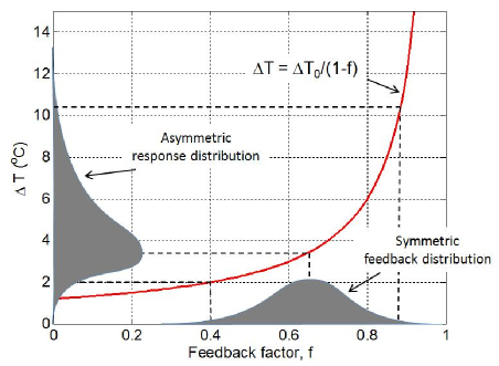
Abbildung 1: Temperature response $\Delta\,T$ as a function of the feedback factor $f$ in a linear climate model; modified after Roe and Baker (2007). In the absence of feedbacks ($f=0$), the response is given by $\Delta\,T=\Delta\,T_{0}=1.2^{o}$C. The response is amplified by feedbacks; it diverges ($\Delta\,T\to\infty$) as $f\to 1$. The shaded areas illustrate the hypothetical symmetric distribution of the feedback factor $f$ and the corresponding asymmetric distribution of the system response $\Delta\,T$. Our study shows that this prominently asymmetric response is only seen in a linear model and is absent in a general nonlinear model (see Fig. 2 below).

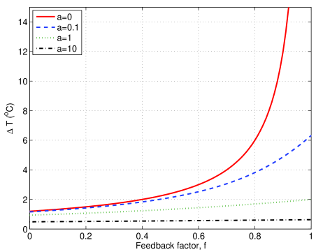
Abbildung 2: Temperature response $\Delta\,T$ as a function of feedback factor $f$ in a nonlinear, quadratic climate model, governed by Eq. (9). The curves correspond (from top to bottom) to increasing values of the magnitude $a=R^{\prime\prime}/2$ of the quadratic term; the values of $a$ for each curve are given in the figure’s legend, in the upper-left corner. The uppermost curve (red) corresponds to $a=0$ and is the same as the one shown in Fig. 1 above. Extreme sensitivity, expressed in the divergence of $\Delta\,T$, is only seen in the linear model; it rapidly vanishes in the nonlinear model, as the nonlinearity factor $a$ increases.

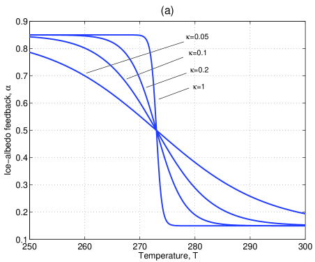
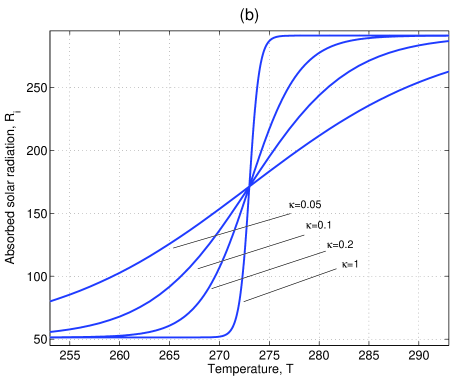
Abbildung 3: Dependence of the absorbed incoming radiation $R_{\rm i}$ on the steepness parameter $\kappa$: (a) ice-albedo feedback $\alpha=\alpha(T;\kappa)$, and (b) absorbed radiation $R_{\rm i}=R_{\rm i}(T;\kappa)$, for different values of $\kappa$; see Eqs. (12) and (13).

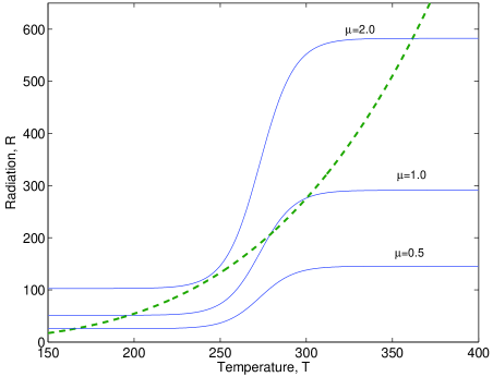
Abbildung 4: Outgoing radiation $R_{\rm o}$ (red, dashed line) and absorbed incoming solar radiation $R_{\rm i}$ (blue, solid lines) for our 0-D energy-balance model (EBM), governed by Eq. (15). The absorbed radiation is shown for $\mu=0.5,1$ and 2.0 (from bottom to top), while $\kappa=0.05$. Notice the existence of one or three intersection points between the $R_{\rm o}$ curve and one of the $R_{\rm i}$ curves, depending on the value of $\mu$; these points correspond to the equilibrium solutions of (15), i.e. to steady-state climates.

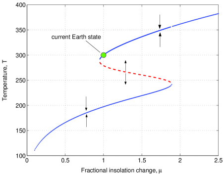
Abbildung 5: Equilibrium solutions of the EBM (15) depending on the fractional change $\mu$ in insolation. Notice the existence of two stable (blue, solid lines) and one unstable (red, dashed line) solution branches. The arrows show the direction in which the global temperature will change after being displaced from a nearby equilibrium state by external forces. The current Earth state corresponds to the upper stable solution at $\mu=1$; in this figure $\kappa=0.05$.

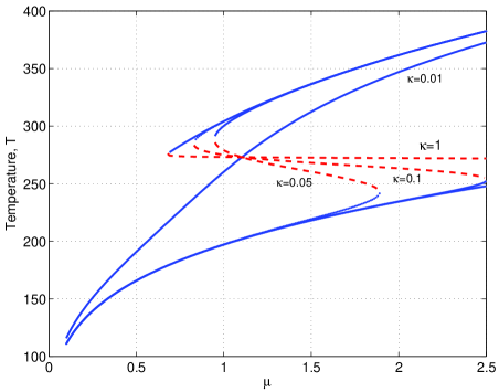
Abbildung 6: Equilibrium solutions of the EBM (15) for ice-albedo feedback functions $\alpha=\alpha(T;\kappa)$ given by Eq. (13) and corresponding to the steepness parameter values $\kappa=0.01,0.05,0.1$ and 1. Notice the deformation of the stable (blue, solid lines) and unstable (red, dashed lines) solution branches: the “coldtipping point moves to the left, away from $\mu=1.0$, as $\kappa$ increases; compare Fig. 3a.