Optical continuous-variable qubit

Abstract

In a new branch of quantum computing, information is encoded into coherent states, the primary carriers of optical communication. To exploit it, quantum bits of these coherent states are needed, but it is notoriously hard to make superpositions of such continuous-variable states. We have realized the complete engineering and characterization of a qubit of two optical continuous-variable states. Using squeezed vacuum as a resource and a special photon subtraction technique, we could with high precision prepare an arbitrary superposition of squeezed vacuum and a squeezed single photon. This could lead the way to demonstrations of coherent state quantum computing.

Among the various physical implementation schemes of quantum information processing (QIP), optical QIP in traveling light fields is a significant contender O'Brien2009 . Used at the nodes of a quantum optical network, it would deliver ultra-high capacity with minimum power in optical communications Waseda2010 and highly secure communications and distributed QIP Kimble2008 ; Briegel1998 ; Bennett1993 surpassing any classical counterpart. Unfortunately, photons do not readily interact with each other, making it quite a task to implement quantum gate elements. One currently feasible scheme is linear optical quantum computing (LOQC), which uses off-line resource states, linear optical processing, and photon-number resolving detection Knill2001 ; Gottesman2001 .There are two approaches to LOQC, the standard one being the single photon scheme, where single photons are used as the physical quantum bits (qubits) Knill2001 . The other is referred to as coherent state quantum computing (CSQC), where two phase-opposite coherent states are used for the qubits, i.e. $\left|\uparrow\right\rangle=\left|\alpha\right\rangle$, $\left|\downarrow\right\rangle=\left|-\alpha\right\rangle$ Cochrane1999 ; Jeong2002 ; Ralph2003 ; Jeong2007b ; Lund2008 .

CSQC is not only effective for exponential speed-up of computations, but also for attaining the ultimate capacity of an optical channel in current network infrastructure where coherent states are the primary carriers. Because coherent states propagate intact, even through lossy channels, simple coherent state-encoding is found to be the optimal transmission strategy Giovannetti2004 . At the same time, the optimal decoding should be fully quantum, and can be implemented by an extension of CSQC Sasaki1998 . Practical implementation of CSQC is still a big challenge, though – one requirement is the availability of arbitrary qubit states as resources. So far, two diagonal states of the qubit $\left|\alpha\right\rangle\pm\left|-\alpha\right\rangle$ – so-called Schrödinger cat states – have been generated in the laboratories Ourjoumtsev2006 ; Neergaard-Nielsen2006 ; Wakui2007 ; Ourjoumtsev2007a ; Takahashi2008 .

We have implemented a setup that is suited for the generation of such arbitrary qubits. For this demonstration, though, we perform the complete engineering of a different, but closely related kind of qubit, namely one with squeezed vacuum and squeezed single-photon states as the basis. The squeezed photon state is in fact very similar to one of the CSQC diagonal qubits, as was utilized in the previous demonstrations of those. To create the arbitrary superposition of the basis states, we use single-photon subtraction from a squeezed vacuum assisted by a coherent displacement operation Takeoka2007 . Photon subtraction is a simple, but powerful technique that has been used for non-classical state generation Ourjoumtsev2006 ; Neergaard-Nielsen2006 ; Wakui2007 ; Ourjoumtsev2007a ; Takahashi2008 , entanglement increase Ourjoumtsev2007 ; Takahashi2010 , and fundamental tests of quantum mechanics Zavatta2009 (see Kim2008a for an overview). A related experiment for engineering of superpositions of the 0-, 1-, and 2-photon states was recently reported Bimbard2009 . In our scheme, in contrast, the state elements of the superposition lie in the infinite dimensional Hilbert space, including many-photon number states. We should also note that spectacular progress in generation of complex, high-photon number states has been made in microwave resonator fields Deleglise2008 ; Hofheinz2009 , but these states are trapped and therefore of limited usefulness.

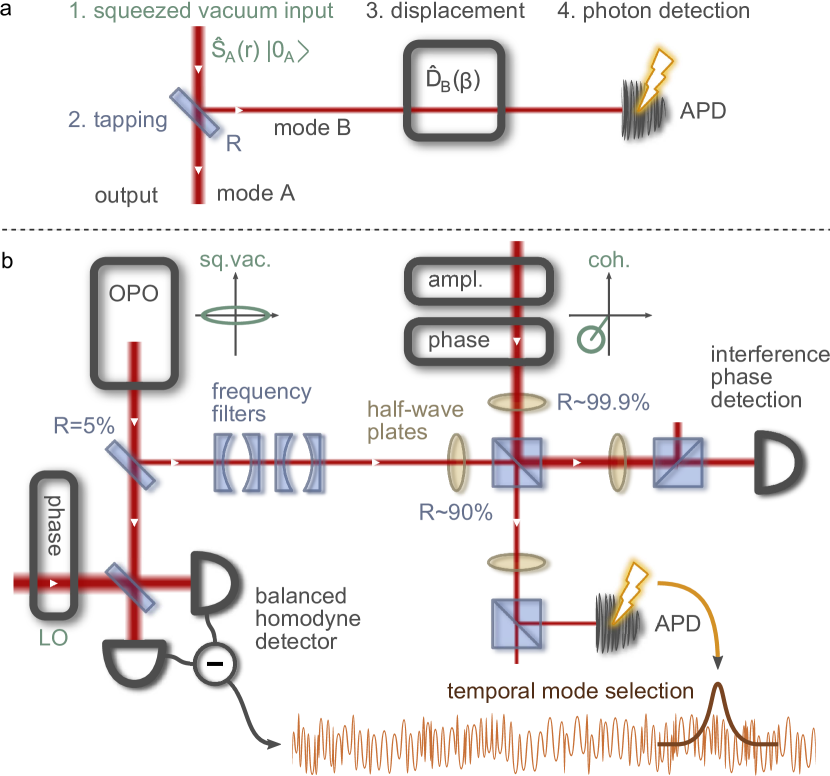
Figure 1: Experiment outline. a) Conceptual schematic. b) Experimental setup. OPO, optical parametric oscillator; R, beam splitter reflectivity; LO, local oscillator; APD, avalanche photo diode.

A simplified schematic is shown in Fig. 1a. The squeezed vacuum state $\hat{S}_{A}(r)\left|0_{A}\right\rangle$ is prepared in mode A, where $\hat{S}_{A}(r)$ represents the squeezing operation with strength $r$. A small fraction $R$ of it is tapped off via a beam splitter as a trigger beam in mode B, subjected to the displacement operation $\hat{D}_{B}(\beta)$, and detected on an avalanche photodiode (APD). Without the displacement operation, the output state conditioned on a click at the APD would be

$$\left\langle 1_{B}\right|\hat{V}_{AB}\hat{S}_{A}(r)\left|0_{AB}\right\rangle\approx-\sqrt{R}\sinh r\hat{S}_{A}(r)\left|1_{A}\right\rangle,$$ (1)

where $\hat{V}_{AB}$ is the beam splitting operator. That is, a photon has been subtracted from the squeezed vacuum state in mode A, which is equivalent to squeezing a single photon. With the inclusion of the displacement operation, this changes to

$$\left\langle 1_{B}\right|\hat{D}_{B}(\beta)\hat{V}_{AB}\hat{S}_{A}(r)\left|0_{AB}\right\rangle\approx\\ \mathcal{N}\big{(}\beta\hat{S}_{A}(r)\left|0_{A}\right\rangle-\sqrt{R}\sinh r\hat{S}_{A}(r)\left|1_{A}\right\rangle\big{)},$$ (2)

with normalization factor $\mathcal{N}$. This superposition originates from the two indistinguishable processes; an APD click comes either from the displacement or from the squeezing, corresponding to the output states $\hat{S}(r)\left|0\right\rangle$ or $\hat{S}(r)\left|1\right\rangle$, respectively. A displacement photon is uncorrelated with the output mode, hence leaving the squeezed vacuum state intact. The superposition weight and phase can be completely controlled by the displacement operation. Each of the two states is composed of several Fock state elements – only even photon numbers for $\hat{S}(r)\left|0\right\rangle$ and odd numbers for $\hat{S}(r)\left|1\right\rangle$. They are orthogonal to each other, so together they constitute a qubit basis and the general output state (2) can therefore be represented on a Bloch sphere as

$$\left|\rho(\theta,\varphi)\right\rangle=\cos\frac{\theta}{2}\hat{S}(r)\left|0\right\rangle+e^{i\varphi}\sin\frac{\theta}{2}\hat{S}(r)\left|1\right\rangle,$$ (3)

with $\varphi=\pi-\arg\beta$ and, after normalization,

$$\cos\frac{\theta}{2}=\frac{|\beta|}{\sqrt{|\beta|^{2}+R\sinh^{2}r}}=\sqrt{\frac{n_{\mathrm{disp}}}{n_{\mathrm{disp}}+n_{\mathrm{sq}}}},$$ (4)

where $n_{\mathrm{disp}}$ ($n_{\mathrm{sq}}$) are the number of photons in mode $B$ originating from the displacement beam (squeezing).

Our experimental setup is shown in detail in Fig. 1b. The input squeezed vacuum states are in a cw beam generated by an optical parametric oscillator (OPO) at a center wavelength of 860nm with a bandwidth $\zeta_{0}/\pi\sim 9$ MHz (FWHM). This cw beam is intuitively a continuous sequence of squeezed light packets, each of which is in a temporal form $\psi(t)=\sqrt{\zeta_{0}}e^{-\zeta_{0}|t|}$ (the squeezing level within these packets is -2.7 dB in our experiment).

After tapping off $R=5\%$ for the trigger, the main part of the light (the output signal) is measured on a homodyne detector for state analysis. The trigger beam is spectrally filtered by two subsequent Fabry-Perot resonators before it is displaced and directed onto a Si APD. The phase space displacement is implemented by overlapping the beam with a weak coherent state on an imbalanced beam splitter Paris1996 . For experimental convenience, we use a combination of half-wave plates (HWP) and a polarizing beam splitter (PBS) which allows for independent tuning of the splitting ratios of the two beams. For the trigger beam, 90% is reflected towards the APD, while only $\sim$0.1% of the displacement beam is transmitted in that direction. The other output mode of the PBS is monitored on a standard linear photodiode for the purpose of locking the displacement phase. The phase monitoring is done with the help of chopped probe light (10 kHz, 20% duty cycle) in both the OPO output and the displacement beam modes, and the locking is controlled by FPGA modules. Apart from this essential displacement part, the setup is mostly identical to that in Refs. Wakui2007 ; Takahashi2008 , where more details are provided.

The time resolution of the trigger signal is on a scale of sub ns, which is almost instantaneous compared with the time scale of the squeezed packets ($\pi/\zeta_{0}\sim 100$ ns). The trigger signal, say at time $t_{1}$, specifies a temporal mode $\psi(t-t_{1})$ of the output state of interest. In the homodyne channel, a continuous photo-current is sampled around the trigger time $t_{1}$, and subsequently integrated over this packet mode function to yield the observed quadrature variable of the field. The specific quadrature to be measured is determined by the phase of the local oscillator (LO) of the homodyne detector. To obtain full information about the output quantum state, we must carry out many homodyne measurements at a range of different LO phases, that is, a tomographic state reconstruction. For each state, 360,000 quadrature points were observed, distributed on 12 different LO phases. The reconstruction was then done by the maximum likelihood method Lvovsky2009 without any correction of measurement losses.

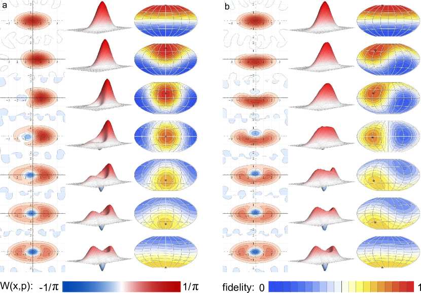
Figure 2: Control of superposition weight. A variety of experimentally generated superposition states where the superposition weight $\theta$ has been swept with the phase $\phi$ fixed at a) 0^∘, and b) $-90^{\circ}$. The left and center panels show the Wigner function as a contour plot and surface plot, respectively. The axes are the $x$- and $p$-quadratures. The right panels show a flattened Bloch sphere with an overlay signifying the fidelity between an ideal qubit (eq. 3) at the given $(\theta,\varphi)$ point and the measured state. The central longitude corresponds to $\varphi=0^{\circ}$, and $\theta=0^{\circ}$ at the north pole. The small circles serve to point out which state we were aiming at. The ideal qubit is taken to have a squeezing parameter $r=0.38$.

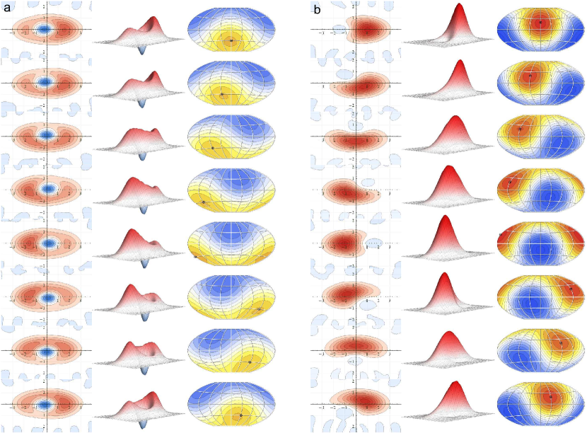
Figure 3: Control of superposition phase. Generated states with the superposition phase $\phi$ swept while keeping the superposition weight $\theta$ constant at a) 135^∘, and b) 60^∘.

A selection of our generated states are presented in Figs. 2 and 3. Each state is represented by its Wigner function as a top-down contour plot and a 3D view, as well as by a Bloch sphere map of the fidelity between the state and the ideal squeezed qubit (3) for all combinations of $\theta$ and $\phi$. To demonstrate the performance of the state engineering, we show in Fig. 2 the control of the superposition weight $\theta$ while keeping the phase constant at a) $\varphi=0^{\circ}$ and b) $\varphi=-90^{\circ}$, and conversely, in Fig. 3 we show the control of the complex phase $\varphi$ for fixed weights of the superposition, a) $\theta=135^{\circ}$ and b) $\theta=60^{\circ}$. In Fig. 2 we see that by increasing the amount of displacement in the trigger channel, $|\beta|$, we can move from the south pole (squeezed photon) to the north pole (squeezed vacuum) of the Bloch sphere along a fixed longitude. While doing that, the negative dip of the Wigner function moves away from the center in a direction determined by the displacement phase. At the same time, the dip becomes shallower and finally disappears as the state approaches the north pole. In Fig. 3, on the other hand, when sweeping the displacement phase, $\mathrm{arg}\beta$, the negative dip circles around the center while the state on the Bloch sphere turns around at a fixed latitude.

From the fidelity maps, we can see that there is a clearly defined qubit state of maximum fidelity in the center of the orange parts of the maps. These maximum points are all quite close to the target states that we aimed for in each qubit realization – these targets are marked by small circles on the fidelity maps. This illustrates the precision of our state control. It is also clear that the obtained fidelities are not as high around the south pole as they are in the north. That is because highly non-classical states with negative Wigner functions, such as the squeezed single photon, are much more fragile and susceptible to losses than, for example, squeezed vacuum.

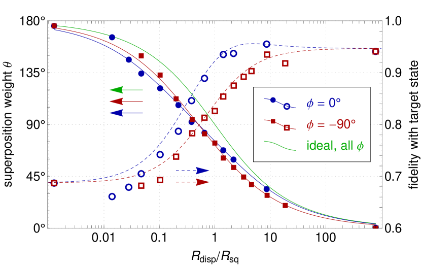
Figure 4: Influence of displacement strength. Experimentally obtained superposition weights (filled points + solid curves, left axis) and fidelities with the intended target states (unfilled points + dashed curves, right axis) versus the APD count rate of displacement photons relative to squeezing photons for two series of measurements with different superposition phase factor. The curves are obtained from a theoretical model with no free parameters, taking into account the various imperfections. The green curve is the relation for the idealized, loss-less case. Note that the extreme data points correspond to count rate ratios of 0 and infinity.

Equation (4) anticipates a direct correspondence between the APD click rates and the resulting superposition weight. The photon number from squeezing (displacement) is directly proportional to the count rate $R_{\mathrm{sq}}$ ($R_{\mathrm{disp}}$) observed when blocking the displacement (trigger) beam before the overlapping PBS, so the relation would read $\theta=2\tan^{-1}(R_{\mathrm{disp}}/R_{\mathrm{sq}})^{-1/2}$. This relation is shown as the green curve in Fig. 4, where also the experimentally obtained $\theta$ (of the ideal qubit with maximum fidelity) as a function of the click rate ratios $R_{\mathrm{disp}}/R_{\mathrm{sq}}$ are plotted. The data points are shown for both the $\varphi=0^{\circ}$ and the $\varphi=-90^{\circ}$ series of state generation. All the points are lying below the theoretical curve. That is because the model in eqs. (2–4) is an idealized picture from which there are several deviations in the actual experiment. In particular, the unavoidable losses in state generation and measurement serve to mix in vacuum which effectively acts to decrease the obtained $\theta$. To more accurately describe the experimental outcomes, we have developed a relatively simple model (see the appendix) which takes into account a more detailed description of the OPO and the trigger filtering, as well as all the inefficiencies of the setup. This model, with no free parameters (except for the squeezing parameter $r$ that is semi-fixed), is also plotted in Fig. 4 and is seen to simulate the measured outcomes very well. Apart from the superposition weights, the figure also shows the fidelities between the measured states and the target states – that is, the fidelity values at the target marks in the Bloch sphere maps of Fig. 2. The state preparation works somewhat better for displacement along the anti-squeezing direction ($\phi=0$) than along the squeezing direction. This can be ascribed to the fact that losses have a larger influence on the squeezed than on the anti-squeezed quadrature. The fidelities are also well described by the theoretical model, although with some smaller discrepancies in the weak-displacement regime.

As these results show, we were able to realize with high precision and relatively high fidelity the complete engineering of a qubit of continuous-variable states. The simple superposition preparation technique demonstrated here can be straight-forwardly applied to generation of coherent state qubits. If the input state instead of squeezed vacuum were one of the ‘cat’ states $\left|\alpha\right\rangle\pm\left|-\alpha\right\rangle$, then the single photon subtraction would change this input into the opposite state $\left|\alpha\right\rangle\mp\left|-\alpha\right\rangle$. Thus, combining this technique with the already existing cat state Takahashi2008 , we should be able to generate an arbitrary superposition of these two cat states. This is equivalent to arbitrary superpositions of the coherent states $\left|\alpha\right\rangle$ and $\left|-\alpha\right\rangle$, i.e. the coherent state qubits that are cornerstones of CSQC. As a side-note, the currently measured basis states, squeezed vacuum and squeezed photon, already have a quite good resemblance with the ‘+’-cat and ‘-’-cat states with fidelities of 81% and 68%, respectively, for a cat-amplitude $\alpha=1.0$. It is also possible to generate larger amplitude cat states by cascading the photon-subtraction Nielsen2007a . The results reported here can therefore lead the way to prototypes of CSQC quantum gates, likely to become important ingredients for attaining the ultimate capacity in future quantum optical networks.

Acknowledgments We would like to acknowledge helpful discussions with Hyunseok Jeong and Chang-Woo Lee.

Appendix: Theoretical model

In this appendix, we outline the theoretical modeling of the quantum states generated in our experiment – a model that fits very well with the observations, as seen in Fig. 4 of the main paper.

We start by recounting the experimental setup and laying out all the relevant parameters. Next, we describe a general Wigner function formalism for calculating the conditional states and relate it to our setting, including imperfections of the displaced photon subtraction. Finally, we specify the actual input Gaussian state, determined by the OPO output correlations, the trigger channel filtering, and our choice of temporal mode functions. To round off, we also include the Wigner function for the ideal squeezed vacuum/squeezed photon qubit – the class of states that we match fidelities against.

Other relevant and more general theoretical descriptions can be found in Refs. app:Suzuki2006 ; app:Sasaki2006a ; app:Takeoka2007 .

$\gamma$	OPO bandwidth	2$\pi\times$4.5 MHz
$\epsilon$	pump level	variable – in this paper, 0.3$\gamma$
$\kappa$	filter bandwidth	$\sim 2\pi\times$25 MHz
$T_{t}$	tapping BS transmission	0.95
$\eta_{A}$	overall efficiency, signal	0.82 ($0.96\times 0.91\times 0.98^{2}\times 0.99\times 0.99$)
$\eta_{B}$	overall efficiency, trigger	$\sim$ 0.1
$R_{\mathrm{sq}}$	click rate, squeezed photons	variable – in this paper, 3600 c/s
$R_{\mathrm{dc}}$	click rate, displacement photons	$\sim$30 c/s
$R_{\mathrm{disp}}$	click rate, dark counts	variable – typically 50-50,000 c/s
$\phi_{\mathrm{disp}}$	displacement angle	variable
$\chi$	displacement mode matching	0.97

Table 1: Model parameters and typical experimental values. The factors of the signal efficiency are: OPO escape, propagation, LO visibility, quantum efficiency, dark noise.

Appendix A EXPERIMENTAL SETTING

Initially, a cw squeezed vacuum is generated by a sub-threshold OPO into mode A. The OPO HWHM bandwidth is $\gamma$ and the pump level is $\epsilon<\gamma$. We align the phase space to have squeezing in the $p$-quadrature. The normal ordered temporal output correlations are then app:Gardiner2000

$$\langle:\!\Delta\hat{x}_{\mathrm{A,ini}}(t)\Delta\hat{x}_{\mathrm{A,ini}}(t^{\prime})\!:\rangle=\frac{\gamma\epsilon}{\gamma-\epsilon}e^{-(\gamma-\epsilon)|t-t^{\prime}|},$$ (5)

$$\langle:\!\Delta\hat{p}_{\mathrm{A,ini}}(t)\Delta\hat{p}_{\mathrm{A,ini}}(t^{\prime})\!:\rangle=-\frac{\gamma\epsilon}{\gamma+\epsilon}e^{-(\gamma+\epsilon)|t-t^{\prime}|}.$$ (6)

The squeezed vacuum is split on a beam splitter with transmission $T_{t}$, being mixed with vacuum from mode B. The transmitted beam is the output signal to be recorded by the homodyne detector whose overall efficiency we denote by $\eta_{A}$ – this efficiency parameter includes internal OPO losses, propagation losses etc. The reflection is sent towards an APD, being displaced on the way (after frequency filtering) by mixing it with a coherent beam. The details of the displacement process are not important: What matters is the rate of APD clicks originating from the squeezed light, $R_{\mathrm{sq}}$, or from the displacement beam, $R_{\mathrm{disp}}$ – a click coming from the squeezed light heralds a photon subtraction in mode A, while a click coming from the displacement beam (uncorrelated with mode A) heralds no action.

Other important parameters are the spatial mode matching between trigger and displacement beam, $\chi$, the dark count rate, $R_{\mathrm{dc}}$, the overall efficiency of mode B (trigger), $\eta_{B}$, the trigger filter bandwidth app:Note1 , $\kappa$, and the phase angle of displacement, $\phi_{\mathrm{disp}}$. The spatial mode matching $\chi$ must be close to 1. If not, the two possible origins of the detected photon are not indistinguishable, leading to a mixed state instead of a superposition.

The parameters used in this model together with their typical experimental values are listed in Table 1. Apart from these, there are also the parameters that define the signal mode function as used in the extraction of the homodyne data: $\gamma_{f}$, $\epsilon_{f}$, and $\kappa_{f}$. These can be chosen freely, but we usually use the experimentally-equivalent values, that is, $\gamma_{f}=\gamma$, $\epsilon_{f}=\epsilon$, $\kappa_{f}=\kappa$.

Appendix B GENERAL OUTPUT STATE FORMALISM

To describe the effect of the photon subtraction, we adopt the Wigner formalism of Ref. app:Molmer2006 . The two-mode state prior to the photon detection event is Gaussian, i.e. it has a Gaussian Wigner function fully determined by the covariance matrix $\Gamma$ and displacement vector $\mathbf{d}$:

$$W_{G}(x_{A},p_{A},x_{B},p_{B})=\frac{1}{\pi^{2}\sqrt{\det\Gamma}}e^{-(\mathbf{x}-\mathbf{d})^{T}\Gamma^{-1}(\mathbf{x}-\mathbf{d})},$$ (7)

with $\mathbf{x}=(x_{A},p_{A},x_{B},p_{B})^{T}$.

To get the state conditional on an APD click in mode B, the Gaussian Wigner function should be multiplied by the Wigner function corresponding to the detection operation and integrated over mode B – this corresponds to $\mathrm{tr}_{B}[\hat{\rho}_{AB}\hat{\Pi}_{B}]$ in the density matrix formulation. For the non-photon number resolving APD, we use the standard on/off operation $\hat{\Pi}_{\mathrm{on}}=\hat{I}-\left|0\right\rangle\left\langle 0\right|$, which has the equivalent Wigner function

$$W_{\mathrm{on}}(x,p)=W_{\mathrm{id}}(x,p)-W_{\mathrm{vac}}(x,p)=\frac{1}{2\pi}-\frac{1}{\pi}e^{-x^{2}-p^{2}}.$$ (8)

The output state conditioned on a displaced 1-photon subtraction is therefore

$$W_{\mathrm{d-1ps}}(x_{A},p_{A})=\\ \mathcal{N}_{\mathrm{out}}\,2\pi\!\!\iint_{-\infty}^{\infty}W_{G}(x_{A},p_{A},x_{B},p_{B})W_{\mathrm{on}}(x_{B},p_{B})\,dx_{B}dp_{B},$$ (9)

with normalization to be determined by integrating the output state.

B.1 Including dark counts and mode matching

If an APD click is a dark count or if it comes from the part of the displacement beam that is not mode-matched to the trigger beam, there is no action on the signal beam and the output state is simply a squeezed vacuum state

$$W_{\mathrm{sq}}(x_{A},p_{A})=\\ 2\pi\!\!\iint_{-\infty}^{\infty}W_{G}(x_{A},p_{A},x_{B},p_{B})W_{\mathrm{id}}(x_{B},p_{B})\,dx_{B}dp_{B}\\ =\iint_{-\infty}^{\infty}W_{G}(x_{A},p_{A},x_{B},p_{B})\,dx_{B}dp_{B}.$$ (10)

If, on the other hand, the click originates from the trigger beam, but from the part which is not mode-matched to the displacement beam, the result will be a normal un-displaced photon subtraction:

$$W_{\mathrm{1ps}}(x_{A},p_{A})=\\ \mathcal{N}_{\mathrm{out}}\,2\pi\!\!\iint_{-\infty}^{\infty}W_{\mathrm{G,nd}}(x_{A},p_{A},x_{B},p_{B})W_{\mathrm{on}}(x_{B},p_{B})\,dx_{B}dp_{B}.$$ (11)

with the un-displaced Gaussian state

$$W_{\mathrm{G,nd}}(x_{A},p_{A},x_{B},p_{B})=\frac{1}{\pi^{2}\sqrt{\det\Gamma}}e^{-\mathbf{x}^{T}\Gamma^{-1}\mathbf{x}}\ .$$ (12)

Let the total count rate be $R=R_{\mathrm{sq}}+R_{\mathrm{disp}}+R_{\mathrm{dc}}$. The final output state is then (with $(x_{A},p_{A})$ temporarily removed)

$$\begin{split}W_{\mathrm{out}}&=\frac{R_{\mathrm{sq}}+R_{\mathrm{disp}}}{R}\bigg{(}\chi W_{\mathrm{d-1ps}}+(1-\chi)\bigg{(}\frac{R_{\mathrm{disp}}}{R_{\mathrm{sq}}+R_{\mathrm{disp}}}W_{\mathrm{sq}}\ +\frac{R_{\mathrm{sq}}}{R_{\mathrm{sq}}+R_{\mathrm{disp}}}W_{\mathrm{1ps}}\bigg{)}\bigg{)}+\frac{R_{\mathrm{dc}}}{R}W_{\mathrm{sq}}\\ &=\chi\frac{R_{\mathrm{sq}}+R_{\mathrm{disp}}}{R}W_{\mathrm{d-1ps}}+(1-\chi)\frac{R_{\mathrm{sq}}}{R}W_{\mathrm{1ps}}+\bigg{(}(1-\chi)\frac{R_{\mathrm{disp}}}{R}+\frac{R_{\mathrm{dc}}}{R}\bigg{)}W_{\mathrm{sq}}\ .\end{split}$$ (13)

B.2 Explicit Wigner function

Any two-mode Gaussian state can – via local operations – be put on the following generic form:

$$\Gamma=\left(\begin{array}[]{cccc}a&0&e&0\\ 0&b&0&f\\ e&0&c&0\\ 0&f&0&d\\ \end{array}\right),\quad\mathbf{d}=\left(\begin{array}[]{c}r\\ s\\ t\\ u\\ \end{array}\right).$$ (14)

By having aligned the squeezing quadrature of the initial state along one of the phase space axes, we have already obtained this form (see next section), where the $x$ and $p$ variables are completely decoupled. We can set $r=s=0$ as displacement only occurs in mode B.

When inserting $\Gamma$ and $\mathbf{d}$ in (7) and carrying out the integrations, we get the following normalized expressions for the three state components of (13):

$$W_{\mathrm{sq}}(x_{A},p_{A}) =\frac{1}{\pi\sqrt{ab}}e^{-\frac{1}{a}x_{A}^{2}-\frac{1}{b}p_{A}^{2}},$$ (15)

$$W_{\mathrm{1ps}}(x_{A},p_{A}) =\frac{1}{1-w}\frac{1}{\pi\sqrt{ab}}e^{-\frac{1}{a}x_{A}^{2}-\frac{1}{b}p_{A}^{2}}$$

$$\quad-\frac{w}{1-w}\frac{1}{\pi\sqrt{a^{\prime}b^{\prime}}}e^{-\frac{1}{a^{\prime}}x_{A}^{2}-\frac{1}{b^{\prime}}p_{A}^{2}},$$ (16)

$$W_{\mathrm{d-1ps}}(x_{A},p_{A}) =\frac{1}{1-w_{d}}\frac{1}{\pi\sqrt{ab}}e^{-\frac{1}{a}x_{A}^{2}-\frac{1}{b}p_{A}^{2}}$$

$$-\frac{w_{d}}{1-w_{d}}\frac{1}{\pi\sqrt{a^{\prime}b^{\prime}}}e^{-\frac{1}{a^{\prime}}(x_{A}-r_{d})^{2}-\frac{1}{b^{\prime}}(p_{A}-s_{d})^{2}},$$ (17)

with

$$a^{\prime} = a-\frac{e^{2}}{1+c},\quad b^{\prime}=b-\frac{f^{2}}{1+d},$$ (18)

$$r_{d} = -\frac{et}{1+c},\quad s_{d}=-\frac{fu}{1+d},$$ (19)

$$w = \frac{2}{\sqrt{(1+c)(1+d)}},$$ (20)

$$w_{d} = \frac{2}{\sqrt{(1+c)(1+d)}}e^{-t^{2}/(1+c)-u^{2}/(1+d)}.$$ (21)

The photon subtracted states are just the difference between two squeezed states. For the total state, we can then gather terms to get

$$\begin{split}W_{\mathrm{out}}(x_{A},p_{A})=&\bigg{(}\chi\frac{R_{\mathrm{sq}}+R_{\mathrm{disp}}}{R}\frac{1}{1-w_{d}}+(1-\chi)\frac{R_{\mathrm{sq}}}{R}\frac{1}{1-w}+\frac{(1-\chi)R_{\mathrm{disp}}+R_{\mathrm{dc}}}{R}\bigg{)}\frac{1}{\pi\sqrt{ab}}e^{-\frac{1}{a}x_{A}^{2}-\frac{1}{b}p_{A}^{2}}\\ &-(1-\chi)\frac{R_{\mathrm{sq}}}{R}\frac{w}{1-w}\frac{1}{\pi\sqrt{a^{\prime}b^{\prime}}}e^{-\frac{1}{a^{\prime}}x_{A}^{2}-\frac{1}{b^{\prime}}p_{A}^{2}}\ \ -\ \ \chi\frac{R_{\mathrm{sq}}+R_{\mathrm{disp}}}{R}\frac{w_{d}}{1-w_{d}}\frac{1}{\pi\sqrt{a^{\prime}b^{\prime}}}e^{-\frac{1}{a^{\prime}}(x_{A}-r_{d})^{2}-\frac{1}{b^{\prime}}(p_{A}-s_{d})^{2}}.\end{split}$$ (22)

Appendix C PHYSICAL DESCRIPTION OF STATE BEFORE TRIGGER DETECTION

In this section, the generalized variables of the covariance matrix and displacement vector in the previous section are related to experimental parameters. The two-mode Gaussian state before the trigger detection has temporal correlations given by the OPO output correlations (5)-(6), by the trigger filtering and by losses. The APD click automatically defines a temporally localized single mode of the trigger beam, and based on the click time, we define a localized mode for the signal beam. Although this mode selection occurs after the actual photon subtraction, it is possible in the model to impose it on the initial Gaussian state, in order to get a time-independent covariance matrix and displacement vector.

C.1 Covariance matrix

The initial time-dependent covariance matrix is modified by the tapping beam splitter, losses, and the mode selection. The handling of covariance matrix transformations is simplified a little by using normal ordering - we do not have to take account of the vacuum contributions until the end.

The initial two-mode time-dependent covariance matrix is

$$:\!\Gamma_{\mathrm{OPO}}(t-t^{\prime})\!:=\left(\begin{array}[]{cccc}:\!\Gamma_{\mathrm{OPO,11}}\!:&0&0&0\\ 0&:\!\Gamma_{\mathrm{OPO,22}}\!:&0&0\\ 0&0&0&0\\ 0&0&0&0\\ \end{array}\right),$$ (23)

with

$$:\!\Gamma_{\mathrm{OPO,11}}\!: = 2\langle:\!\Delta\hat{x}_{\mathrm{A,ini}}(t)\Delta\hat{x}_{\mathrm{A,ini}}(t^{\prime})\!:\rangle,$$ (24)

$$:\!\Gamma_{\mathrm{OPO,22}}\!: = 2\langle:\!\Delta\hat{p}_{\mathrm{A,ini}}(t)\Delta\hat{p}_{\mathrm{A,ini}}(t^{\prime})\!:\rangle.$$ (25)

The tapping beam splitter, represented by the matrix $V(T_{t})$, transforms it to

$$:\!\Gamma_{\mathrm{bs}}(t-t^{\prime})\!:=V(T_{t}):\!\Gamma_{\mathrm{ini}}(t-t^{\prime})\!:V(T_{t})^{T}.$$ (26)

To obtain the state within the selected temporal mode, we integrate the quadrature variables over the relevant filter functions, $f_{A}(t),f_{B}(t)$, for example,

$$\hat{x}_{A}=\int_{-\infty}^{\infty}f_{A}(t)\hat{x}_{\mathrm{A,bs}}(t)dt.$$ (27)

When calculating the elements of the covariance matrix $\Gamma$, we can move the integration outside the expectation values, e.g.

$$\begin{split}:\!\Gamma_{13}\!:&=2\langle:\!\Delta\hat{x}_{A}\Delta\hat{x}_{B}\!:\rangle\\ &=2\langle:\!\int\!\!f_{A}(t)\Delta\hat{x}_{\mathrm{A,bs}}(t)dt\int\!\!f_{B}(t^{\prime})\Delta\hat{x}_{\mathrm{B,bs}}(t^{\prime})dt^{\prime}\!:\rangle\\ &=\int\!\!f_{A}(t)f_{B}(t^{\prime})\ 2\langle:\!\Delta\hat{x}_{\mathrm{A,bs}}(t)\Delta\hat{x}_{\mathrm{B,bs}}(t^{\prime})\!:\rangle dtdt^{\prime}\\ &=\int\!\!f_{A}(t)f_{B}(t^{\prime}):\!\Gamma_{\mathrm{bs,13}}(t-t^{\prime})\!:dtdt^{\prime}.\end{split}$$ (28)

Losses in both modes, as well as the trigger frequency filtering can be incorporated in the filter functions (see later). Therefore, the final matrix is

$$:\!\Gamma\!:\ =\iint\mathbf{f}(t)^{T}:\!\Gamma_{\mathrm{bs}}(t-t^{\prime})\!:\mathbf{f}(t^{\prime})\,dtdt^{\prime},$$ (29)

with $\mathbf{f}(t)=\mathrm{diag}(f_{A}(t),f_{A}(t),f_{B}(t),f_{B}(t))$, and, remembering to put back the vacuum:

$$\Gamma=\ :\!\Gamma\!:+\Gamma_{\mathrm{vac}}.$$ (30)

C.2 Displacement vector

With a displacement $\hat{D}_{B}(\beta)=\hat{D}_{B}\big{(}|\beta|e^{i\phi_{\mathrm{disp}}}\big{)}$ in mode B, the displacement vector is

$$\mathbf{d}=\sqrt{2}|\beta|\ (0,0,\cos\phi_{\mathrm{disp}},\sin\phi_{\mathrm{disp}})^{T}.$$ (31)

The photon number in the mode due to this displacement is of course $n_{\mathrm{disp}}=|\beta|^{2}$. On the other hand, from $n=(\langle:\!\Delta\hat{x}^{2}\!:\rangle+\langle:\!\Delta\hat{p}^{2}\!:\rangle)/2$, the photon number due to the squeezing can be obtained as

$$n_{\mathrm{sq}}=\frac{1}{4}\left(:\!\Gamma_{33}\!:+:\!\Gamma_{44}\!:\right).$$ (32)

The photon numbers are not directly experimentally accessible, but they are proportional to the detected APD click rates, so we can get $|\beta|$ and the displacement vector in terms of these rates:

$$|\beta|=\sqrt{\frac{n_{\mathrm{disp}}}{n_{\mathrm{sq}}}n_{\mathrm{sq}}}=\sqrt{\frac{R_{\mathrm{disp}}}{R_{\mathrm{sq}}}\frac{:\!\Gamma_{33}\!:+:\!\Gamma_{44}\!:}{4}}\ ,$$ (33)

$$\mathbf{d}=\sqrt{\frac{R_{\mathrm{disp}}}{R_{\mathrm{sq}}}\frac{:\!\Gamma_{33}\!:+:\!\Gamma_{44}\!:}{2}}\ (0,0,\cos\phi_{\mathrm{disp}},\sin\phi_{\mathrm{disp}})^{T}\ .$$ (34)

C.3 Mode functions

In the approach taken here, the filter functions play two different roles:

1. To model the physical effect on the correlation matrix by losses and trigger filtering.

2. To describe the actual observed temporal mode.

#2 is the original meaning of the mode function, but #1 can be included very nicely.

For the signal (mode A), the observed mode is the temporal filter applied to the raw homodyne data in post-processing. This can be chosen freely, but we always use the experimentally most reasonable function which is

$$\psi_{A}(t)=\sqrt{\mathcal{N}_{A}}\left(\frac{e^{-\gamma|t|}}{\gamma}-\frac{e^{-\kappa|t|}}{\kappa}\right),$$ (35)

with normalization $\mathcal{N}_{A}=\gamma^{3}\kappa^{3}(\gamma+\kappa)/(\gamma^{4}+\gamma^{3}\kappa-4\gamma^{2}\kappa^{2}+\gamma\kappa^{3}+\kappa^{4})$. This is the double-sided exponential from the OPO output correlations, smoothened by the frequency filtering of the trigger. Including the overall signal efficiency gives the filter function

$$f_{A}(t)=\sqrt{\eta_{A}}\psi_{A}(t).$$ (36)

The APD detection time is very short relative to the correlation time, so the temporal mode can be taken to be a delta function:

$$\psi_{B}(t)=\delta(t).$$ (37)

The frequency filtering, however, has the effect that the photons arriving at the APD has been delayed relative to their correlated twins in the signal path. This can be taken into account by convoluting the mode function with the filter response, which gives (assuming the single Lorentzian filter)

$$f_{B}(t)=\sqrt{2\kappa\eta_{B}}e^{\kappa t}\ ,\quad\text{for}\ t\leq 0\ \text{and 0 otherwise}.$$ (38)

The overall trigger efficiency was also included in the filter function.

Both filter functions assumes a photon click at time $t=0$. Due to the inclusion of losses, they are not normalized to 1.

Appendix D IDEAL SQUEEZED QUBIT

When we compare the experimentally obtained or theoretically predicted states with the ideal squeezed qubit, we calculate the overlap (fidelity) between the Wigner function of these states and the Wigner function of the ideal squeezed qubit app:Note2 . Given parameters $r$ (squeezing parameter), $\theta$ and $\phi$ (Bloch vector), the ideal squeezed qubit has the state ket

$$\left|\mathrm{SQ}\right\rangle=\cos\frac{\theta}{2}\hat{S}(r)\left|0\right\rangle+e^{i\varphi}\sin\frac{\theta}{2}\hat{S}(r)\left|1\right\rangle,$$ (39)

For the calculation of the Wigner function, $W_{\mathrm{SQ}}(x,p)=(2\pi)^{-1}\int e^{iyp}\langle x-y/2\left|\mathrm{SQ}\right\rangle\left\langle\mathrm{SQ}\right|x+y/2\rangle dy$, we need the wave functions of the squeezed vacuum and the squeezed photon:

$$\left\langle x\right|\hat{S}(r)\left|0\right\rangle =(\pi e^{2r})^{-1/4}e^{-x^{2}/2e^{2r}},$$ (40)

$$\left\langle x\right|\hat{S}(r)\left|1\right\rangle =\left\langle x\right|\frac{1}{\sinh r}\hat{a}\hat{S}(r)\left|0\right\rangle$$

$$=\frac{1}{\sqrt{2}\sinh r}\left(x+\frac{d}{dx}\right)\left\langle x\right|\hat{S}(r)\left|0\right\rangle$$

$$=\sqrt{\frac{2}{\sqrt{\pi}e^{3r}}}\,xe^{-x^{2}/2e^{2r}}.$$ (41)

This gives the following expression for the squeezed qubit Wigner function:

$$W_{\mathrm{SQ}}(x,p)=\frac{1}{\pi}e^{-e^{-2r}x^{2}-e^{2r}p^{2}}\bigg{(}\!\cos\theta+(1-\cos\theta)\Big{(}\frac{x^{2}}{e^{2r}}+\frac{p^{2}}{e^{-2r}}\Big{)}+\sqrt{2}\Big{(}\cos\phi\frac{x}{e^{r}}+\sin\phi\frac{p}{e^{-r}}\Big{)}\sin\theta\bigg{)}.$$ (42)

References

- (1) J. L. O’Brien, A. Furusawa, and J. Vučković, Nature Photonics 3, 687 (2009)
- (2) A. Waseda, M. Takeoka, M. Sasaki, M. Fujiwara, and H. Tanaka, J. Opt. Soc. Am. B 27, 259 (2010)
- (3) H. J. Kimble, Nature 453, 1023 (2008)
- (4) H.-J. Briegel, W. Dür, J. I. Cirac, and P. Zoller, Phys. Rev. Lett. 81, 5932 (1998)
- (5) C. H. Bennett, G. Brassard, C. Crépeau, R. Jozsa, A. Peres, and W. K. Wootters, Phys. Rev. Lett. 70, 1895 (1993)
- (6) E. Knill, R. Laflamme, and G. J. Milburn, Nature 409, 46 (2001)
- (7) D. Gottesman, A. Kitaev, and J. Preskill, Phys. Rev. A 64, 012310 (2001)
- (8) P. Cochrane, G. Milburn, and W. Munro, Phys. Rev. A 59, 2631 (1999)
- (9) H. Jeong and M. Kim, Phys. Rev. A 65, 042305 (2002)
- (10) T. C. Ralph, A. Gilchrist, G. J. Milburn, W. J. Munro, and S. Glancy, Phys. Rev. A 68, 042319 (2003)
- (11) H. Jeong and T. Ralph, in Quantum Information with Continuous Variables of Atoms and Light, edited by N. Cerf, G. Leuchs, and E. Polzik (Imperial College Press, London, 2007) Chap. 9
- (12) A. Lund, T. Ralph, and H. Haselgrove, Phys. Rev. Lett. 100, 030503 (2008)
- (13) V. Giovannetti, S. Guha, S. Lloyd, L. Maccone, J. Shapiro, and H. Yuen, Phys. Rev. Lett. 92, 027902 (2004)
- (14) M. Sasaki, T. Sasaki-Usuda, M. Izutsu, and O. Hirota, Phys. Rev. A 58, 159 (1998)
- (15) A. Ourjoumtsev, R. Tualle-Brouri, J. Laurat, and P. Grangier, Science 312, 83 (2006)
- (16) J. S. Neergaard-Nielsen, B. M. Nielsen, C. Hettich, K. Mølmer, and E. S. Polzik, Phys. Rev. Lett. 97, 083604 (2006)
- (17) K. Wakui, H. Takahashi, A. Furusawa, and M. Sasaki, Opt. Express 15, 3568 (2007)
- (18) A. Ourjoumtsev, H. Jeong, R. Tualle-Brouri, and P. Grangier, Nature 448, 784 (2007)
- (19) H. Takahashi, K. Wakui, S. Suzuki, M. Takeoka, K. Hayasaka, A. Furusawa, and M. Sasaki, Phys. Rev. Lett. 101, 233605 (2008)
- (20) M. Takeoka and M. Sasaki, Phys. Rev. A 75, 064302 (2007)
- (21) A. Ourjoumtsev, A. Dantan, R. Tualle-Brouri, and P. Grangier, Phys. Rev. Lett. 98, 030502 (2007)
- (22) H. Takahashi, J. S. Neergaard-Nielsen, M. Takeuchi, M. Takeoka, K. Hayasaka, A. Furusawa, and M. Sasaki, Nature Photonics, DOI:10.1038/nphoton.2010.1(2010)
- (23) A. Zavatta, V. Parigi, M. Kim, H. Jeong, and M. Bellini, Phys. Rev. Lett. 103, 140406 (2009)
- (24) M. S. Kim, J. Phys. B: At. Mol. Opt. Phys 41, 133001 (2008)
- (25) E. Bimbard, N. Jain, A. MacRae, and A. Lvovsky, Nature Photonics, DOI:10.1038/nphoton.2010.6(2010)
- (26) S. Deléglise, I. Dotsenko, C. Sayrin, J. Bernu, M. Brune, J.-M. Raimond, and S. Haroche, Nature 455, 510 (2008)
- (27) M. Hofheinz, H. Wang, M. Ansmann, R. C. Bialczak, E. Lucero, M. Neeley, A. D. O’Connell, D. Sank, J. Wenner, J. M. Martinis, and A. N. Cleland, Nature 459, 546 (2009)
- (28) M. Paris, Phys. Lett. A 217, 78–80 (1996)
- (29) A. Lvovsky and M. Raymer, Rev. Mod. Phys. 81, 299 (2009)
- (30) A. E. B. Nielsen and K. Mølmer, Phys. Rev. A 76, 043840 (2007)

References

- (1) S. Suzuki, K. Tsujino, F. Kannari, M. Sasaki, Opt. Comm. 259, 758 (2006).
- (2) M. Sasaki and S. Suzuki, Phys. Rev. A 73, 043807 (2006).
- (3) M. Takeoka and M. Sasaki, Phys. Rev. A 75, 064302 (2007).
- (4) C. W. Gardiner, P. Zoller, Quantum Noise, Springer-Verlag, Berlin (2000).
- (5) The trigger filtering consists of two Fabry-Perot cavities, each with a Lorentzian transmission spectrum. However, one cavity is considerably narrower than the other, so we model the total effect of the filtering as a single Lorentzian filter with a bandwidth slightly lower than that of the narrowest cavity.
- (6) K. Mølmer, Phys. Rev. A 73, 063804 (2006).
- (7) The experimental reconstruction method actually gives a density matrix instead of a Wigner function, so for the measured states we calculate fidelity by the trace of the density matrix products instead. This is equivalent to the Wigner function overlap.