Anomalous Hall effects and electron polarizability

Abstract

A theory of the anomalous and spin Hall effects, based on the space distribution of the current densities, is presented. Spin-orbit coupling gives rise to a space separation of the mass centers, as well as a current density separation of the quasiparticle states having opposite group velocities. It is shown that this microscopic property is essential for existence of both Hall effects.

It has been known for more than a century that a ferromagnetic material exhibits, in addition to the standard Hall effect when placed in a magnetic field, an extraordinary Hall effect which does not vanish at zero magnetic field. The theory of this so-called anomalous Hall effect (AHE) has a long and confusing history, with different approaches giving in some cases conflicting results. While more recent calculations have somewhat unified the different approaches and clarified the situation, it is still an active topic of research (see Ref. [Nagaosa2009, ] for a recent review). Closely related to the AHE is the spin Hall effect, represented by spin accumulation on the edges of a current carrying sample spin_Hall_1 ; spin_Hall_2 .

It is generally accepted that the anomalous and spin Hall effects are induced by spin-orbit coupling. It was first suggested by Karplus and Luttinger Karplus in 1954 to explain anomalous Hall effect observed on ferromagnetic crystals. Their analysis leads to the scattering independent off-diagonal components of the conductivity, which are assigned to the so-called ”intrinsic” effect. Later, theories of this effect based on several specific models have been developed Miyazawa ; Onoda . As has been recently shown it is accompanied by strong orbital Hall effect Shindou ; Kontani . The conductivity is also affected by the scattering, which in the presence of spin-orbit coupling gives rise to so called side-jump Berger and skew scattering Smit ; Luttinger_58 ; Sinitsyn . These also lead to anomalous Hall effect, called ”extrinsic”. The best quantitative agreement with experimental observations has been obtained with semi-classical transport theory Niu , leading to the Berry phase correction to the group velocity. For Fe crystals Jungw_2 it gives an anomalous conductivity $\sim 750\;\Omega^{-1}$ cm^-1 while a value approaching $1000\;\Omega^{-1}$ cm^-1 has been observed.

It is the goal of this letter to shed light on AHE using a novel point of view. Our approach is based on the analysis of the space distribution of local current densities, and it is simple and rather intuitive. We will show that the anomalous Hall conductivity is related to the spatial separation of the mass centers of states with opposite velocities. This confirms the interpretation of AHE in ferromagnetic systems as a consequence of the periodic field of electric dipoles (electric polarizability) induced by the applied current Karplus ; Adams ; Fivaz , despite the fact that the original arguments were not convincing Berger . We will also show that in non-magnetic systems, the spin-orbit coupling leads to a periodic variation of the spin polarizability of the current densities in the transport regime. This effect can be viewed as an internal spin Hall effect. For the sake of simplicity, we limit our consideration to crystalline structures invariant under space inversion.

Current density distribution is closely related to the orbital magnetization of solids. In zero magnetic field it has its origin in the orbital magnetic moment of atomic states. Ignoring spin effects, atomic wave functions in spherical polar-coordinate system can be written as

$$\Psi^{(at)}_{\alpha}(r,\theta,\phi)\,=\,f_{\alpha}(r,\theta)\,\frac{e^{im\phi}}{\sqrt{2\pi}}\qquad,\quad\alpha\,\equiv\,n,l,m\;,$$ (1)

where $m$ is the so called magnetic quantum number, with $m=0,\pm 1,\cdots$, and $|m|\leq l$. It determines the magnetic moment along the $\hat{z}$ direction

$$M_{z}(\alpha)\equiv-\frac{e}{2c}\langle\alpha|\left(\vec{r}\times\vec{v}\right)_{z}|\alpha\rangle\equiv-\frac{m}{|m|}\,\frac{\pi R_{\alpha}^{2}}{c}\;\left|j_{\alpha}\right|\;,$$ (2)

where $e$ denotes absolute value of the electron charge and $\vec{v}$ stands for velocity operator. The last expression represents a classical analogy with $j_{\alpha}$ being the current flowing on a circular loop of the radius $R_{\alpha}$. Because of the energy degeneracy in $m$ the total orbital magnetic moment vanishes. However, spin-orbit coupling together with exchange interaction remove this degeneracy giving rise to non-zero magnetic moment.

Within a mean field approach the electron properties are controlled by a single electron Hamiltonian $H$ containing two additive terms $H_{so}$ and $H_{z}$ representing spin-orbit coupling and an effective Zeeman-like spin splitting due to the exchange interaction, respectively:

$$H\,=\,\frac{p^{2}}{2m_{0}}\,+\,V(\vec{r})\,+\,H_{so}\,+\,H_{z}\;,$$ (3)

with $m_{0}$ being free electron mass, $V(\vec{r})$ denotes the crystalline potential, $\vec{p}$ is momentum operator and

$$H_{so}\,=\,\frac{\lambda_{c}^{2}}{4\hbar}\,\vec{\sigma}\cdot\left[\vec{\nabla}V(\vec{r})\times\vec{p}\,\right]\;\;,\;\;H_{z}\,=\,-\,\mu_{B}\,\vec{B}_{\rm eff}\cdot\vec{\sigma}\,,$$ (4)

where $\lambda_{c}$ denotes an effective Compton length, and elements of the vector $\vec{\sigma}$ are Pauli matrices. Strength of the Zeeman-like splitting is controlled by the product of the Bohr magneton $\mu_{B}$ and the parameter $\vec{B}_{\rm eff}$ representing an effective magnetic field. The corresponding velocity operator reads

$$\vec{v}\,=\,\frac{\vec{p}}{m_{0}}\,+\,\frac{\lambda_{c}^{2}}{4\hbar}\,\vec{\sigma}\times\vec{\nabla}V(\vec{r})\;.$$ (5)

Eigenfunctions are spinors with two components, and since spin-orbit coupling does not destroy translation symmetry they are of the Bloch form. Energy spectrum $E_{\alpha}(k)$ is a function of the wave vector $\vec{k}$, with $\alpha$ being a band index, now including also, in addition to atomic orbital numbers, a spin number. Eigenfunctions are of the following form

$$|\alpha,\vec{k}\rangle\equiv\Psi_{\alpha,\vec{k}}(\vec{r})=\frac{e^{i\vec{k}\vec{r}}}{\sqrt{8\pi^{3}}}\,u_{\alpha}(\vec{k},\vec{r})\,,$$ (6)

and velocity expectation values are

$$\vec{v}_{\alpha}(\vec{k})=\frac{1}{\hbar}\vec{\nabla}_{\vec{k}}E_{\alpha}(\vec{k})\,.$$ (7)

Spinors $u_{\alpha}(k,\vec{r})$ are periodic functions of the lattice translation vectors. Assumed invariance under space inversion results in following $\vec{k}$-space symmetry: $E_{\alpha}(\vec{k})=E_{\alpha}(-\vec{k})$ and $v_{\alpha}(\vec{k})=-v_{\alpha}(-\vec{k})$.

In order to analyze the role of the space distribution of the current densities, it is illustrative to present first the results for a simple model of a linear chain of atomic orbitals. It is assumed that this chain is forming a one-dimensional lattice along $\hat{x}$ direction with a period $a$. Model parameter will be chosen to satisfy conditions for which the tight-binding approach is applicable. Energy bands originated in overlap of atomic states $|\alpha\rangle$ will be denoted by the corresponding magnetic quantum number $m$. To model a ferromagnetic state, we assume that the effective field $\vec{B}_{\rm eff}$ is parallel with $\hat{z}$ direction and it is strong enough to ensure spin orientation along $\pm\hat{z}$ direction with $s_{z}=\pm 1/2$ being good quantum numbers. We have obtained numerical results by diagonalizing the single particle Hamiltonian for a two-dimensional separable chain potential

$$V(x,y)\,=\,-\,V_{0}\cos(2\pi x/a)+m_{0}\Omega_{0}^{2}y^{2}/2\;.$$ (8)

Note that adding a $z$-dependent potential would not affect the current distribution of the considered model system. The parameters have been chosen to be in the tight-binding regime, i.e. to fully separate the studied band from the other energy bands (we used $2m_{0}a^{2}V_{0}/\hbar^{2}=75.0$, $m_{0}\Omega_{0}^{2}a^{2}=1.4\times 4\pi^{2}V_{0}$ and $\pi\lambda_{c}^{2}/a^{2}=0.015$).

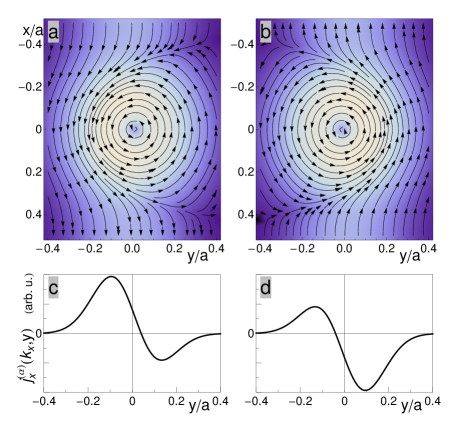
Figure 1: (color online) Current distributions for an energy band given by a chain of atomic states with spin $s_{z}=1/2$ and $m=-1$ for $k_{x}=1.5/a$ (a,c) and $k_{x}=-1.5/a$ (b,d). In a and b, the arrows indicate the direction of the current, and a lighter background indicates a larger current. In c and d the averaged current densities $j_{x}^{\alpha}(k_{x},y)$ are shown.

Typical current density distribution within the unit cell for the Bloch states $|\alpha,k_{x}\rangle$ and $|\alpha,-k_{x}\rangle$ are shown in Figs. 1a and 1b, respectively. One observes circulating currents forming vortices, which have the same orientation for both cases. This orientation coincides with the orientation of the circulating current of the atomic orbitals. In addition to this circulating current, there is a direct current flow, with opposite sign for the two cases. Corresponding total current and its direction is just determined by the velocity expectation value, $-ev_{x}^{\alpha}(k_{x})$. Note that these current flows are spatially separated in the two cases (they are on opposite sides of the circulating current). The current densities averaged over $x$ and $z$ coordinates,

$$j_{x}^{\alpha}(k_{x},y)=-e\int\int\Psi_{\alpha,k_{x}}^{+}(\vec{r})\,v_{x}\Psi_{\alpha,k_{x}}(\vec{r})\,dx\,dz\,,$$ (9)

clearly demonstrate the above mentioned spatial separation of the currents having opposite velocity directions, as shown on Figs. 1c and 1d.

This space separation of currents flowing in opposite directions is closely related to the mass-center separation $\Delta Y_{\alpha}(k_{x})$ of states $|\alpha,k_{x}\rangle$ and $|\alpha,-k_{x}\rangle$ with $k_{x}$ being consider as positive, $k_{x}>0$. For the considered model potential, Eq. (8), the $y$-component of the force operator reads

$$F_{y}\,\equiv\,\frac{1}{i\hbar}\,[p_{y},H]\,=\,-\,m_{0}\Omega_{0}^{2}y\,+\,2s_{z}\,\frac{\lambda_{c}^{2}}{4\hbar}\,m_{0}\Omega_{0}^{2}\,p_{x}\;.$$ (10)

In a stationary state the force expectation values has to vanish. Using the relation between $p_{x}$ and $v_{x}$ given by Eq. (5) we get

$$\Delta Y_{\alpha}(k_{x})=2s_{z}\,\frac{\lambda_{c}^{2}m_{0}}{4\hbar}\left[1-\left(\frac{\lambda_{c}^{2}m_{0}}{4\hbar}\right)^{2}\Omega_{0}^{2}\right]^{-1}\!2v_{x}^{\alpha}(k_{x})\;.$$ (11)

In the limiting case of vanishing spin-orbit coupling $\Delta Y_{\alpha}(k_{x})\rightarrow 0$ and sum of the current densities $j_{x}^{\alpha}(k_{x},y)+j_{x}^{\alpha}(-k_{x},y)$ approaches zero as well.

Non-zero total current appears if there is different occupation of states with opposite velocities which can be characterized by the chemical potential difference $\Delta\mu$. It can be related to the electric field along $\hat{y}$ direction, ${\cal{E}}_{y}=\Delta\mu/(e|\Delta Y_{\alpha}(k_{F})|)$, with $\Delta Y_{\alpha}(k_{F})$ being the mass-center separation of quasiparticles having opposite velocities at the Fermi energy $E_{F}=\mu$. Within linear response approach the resulting current at zero temperature reads

$$J_{x}^{\alpha}(\mu)=-\frac{e}{h}\frac{v_{x}^{\alpha}(k_{F})-v_{x}^{\alpha}(-k_{F})}{\left|v_{x}^{\alpha}(k_{F})\right|}\,\Delta\mu=-\frac{e^{2}}{h}\,\Delta Y_{\alpha}(k_{F})\,{\cal{E}}_{y}\;.$$ (12)

Because of the non-zero separation $\Delta Y_{\alpha}(k_{F})$ and non-equal occupation of states with opposite velocities the applied current is giving rise an electric dipole moment, i.e. a charge polarization is induced.

For the later use, let us express current $J_{x}^{\alpha}(\mu)$ in terms of the following quantity

$$\frac{\vec{P}_{\alpha}(\vec{k})}{\Omega_{\rm ws}}\,\equiv\,-\,\frac{e}{c}\,\langle\alpha,\vec{k}|\vec{r}|\alpha,\vec{k}\rangle\times\vec{v}_{\alpha}(\vec{k})\;,$$ (13)

where $\Omega_{\rm ws}$ defines a unit cell volume. Evaluation of the following expression

$$J_{x}^{\alpha}(\mu)=-\frac{ec{\cal{E}}_{y}}{2\pi\Omega_{\rm ws}}\int\limits_{-\pi/a}^{+\pi/a}\!\!\delta(E_{\alpha}(k_{x})-\mu)\,\left[\vec{P}_{\alpha}(k_{x})\right]_{z}dk_{x}\;,$$ (14)

immediately gives the above result, Eq. (12), since velocity expectation value along $\hat{y}$ direction vanishes. The above defined quantity, Eq. (13), is the part of the orbital magnetic moment within each of the unit cells which gives rise an electric dipole moment in the current carrying regime. For this reason it will be called as the orbital polarization moment.

Generalization of the above treatment to a three-dimensional system is straightforward. Velocity expectation values have non-zero component also along $\hat{y}$ direction and they contribute to the orbital polarization moment defined by Eq. (13). The resulting contribution of the band $\alpha$ to the Hall conductivity component $\sigma_{xy}$ can thus be written as follows

$$\sigma_{xy}^{(\alpha)}(\mu)=-\frac{ec}{8\pi^{3}\Omega_{\rm ws}}\int\limits_{\rm BZ}\!\!\delta(E_{\alpha}(\vec{k})-\mu)\,\left[\vec{P}_{\alpha}(\vec{k})\right]_{z}d^{3}k\,,$$ (15)

where integration is limited to the Brillouin zone and $\Omega_{\rm ws}$ now denotes volume of the Wiegner-Seitz cell. Inserting for $\vec{P}_{\alpha}(\vec{k})$ and $\vec{v}_{\alpha}(\vec{k})$ their explicit forms, Eq. (13) and Eq. (7), respectively, and using equality

$$\langle\alpha,\vec{k}|\vec{r}\,|\alpha,\vec{k}\rangle=-{\rm Im}\int\limits_{\Omega_{\rm ws}}\!u^{+}_{\alpha}(\vec{k},\vec{r})\left(\vec{\nabla}_{\vec{k}}u_{\alpha}(\vec{k},\vec{r})\right)d^{3}r\,,$$ (16)

already derived by Karplus and Luttinger Karplus , the integration per parts gives the well known expression for the Hall conductivity of Bloch electrons

$$\sigma_{xy}(\mu)=-\frac{e^{2}}{4\pi^{2}h}\sum_{\alpha}\int\limits_{\rm BZ}\!\!f_{0}\left(E_{\alpha}(\vec{k})\right)\,\left[\vec{\Omega}_{\alpha}(\vec{k})\right]_{z}d^{3}k\,.$$ (17)

Here $f_{0}(E)$ stands for zero-temperature Fermi-Dirac distribution function and the Berry phase curvature $\vec{\Omega}_{\alpha}(\vec{k})$ defined by the periodic part of Bloch functions, $u_{\alpha}(\vec{k},\vec{r})$, reads

$$\vec{\Omega}_{\alpha}(\vec{k})\,=\,-\,{\rm Im}\,\left\langle\,\vec{\nabla}_{\vec{k}}\,u_{\alpha}(\vec{k},\vec{r})\,\left|\times\right|\,\vec{\nabla}_{\vec{k}}\,u_{\alpha}(\vec{k},\vec{r})\,\right\rangle\,.$$ (18)

Our description of the anomalous Hall effect based on charge polarization effect is thus equivalent to the approach based on the Berry phase correction Niu .

For completeness, we must note that for the three-dimensional case, computing the quantity $\Delta Y$, representing the mass-center separation of states having opposite velocities along $\hat{x}$ direction, is not as easy as it was for the single atomic chain. It requires to express eigenfunctions in a mixed representation, to preserve the Bloch form along the $\hat{x}$ direction, while using Wannier representation along perpendicular directions. The Wannier representation gives functions which are bounded along the $\hat{y}$ direction, allowing to compute $\Delta Y$. Although the explicit form of $\Delta Y$ is not simple, the main features are qualitatively the same as those presented for the single chain.

Conductivity can directly be measured on samples having Corbino disc geometry. This arrangement can be modelled by considering a strip with periodic boundary conditions along $\hat{x}$ direction and current contacts attached to the strip edges allowing to apply current along $\hat{y}$ direction. It induces gradient of the electro-chemical potential along $\hat{y}$ direction and consequently it gives rise to the local charge polarization. As a result, Hall current is induced. Intra band scattering ensuring finite conductivity across the strip is naturally of the side-jump character. This type of scattering does not affect Hall conductivity which is given as the sum of the additive band contributions defined by Eq. (15) or Eq. (17). However, inter band scattering which is generally of the skew character can affect Hall conductivity significantly. These features of the anomalous conductivity directly follows from the analysis based on quantum theory of the linear response, Kubo formula. Although the derivation is straightforward, it is quite lengthy and will be thus presented in a separate publication.

The relation we have presented here between the charge polarization and the anomalous Hall effect is similar to the discussion of Hall conductivity of Bloch electrons in rational quantizing magneticgv fields in terms of charge polarization.polarizability_08 However, in that case the physical picture is strongly affected by chiral magnetic edge states.

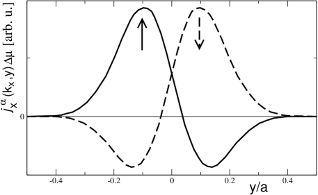
Figure 2: Transport current densities $j_{x}^{\alpha}(k_{x},y)\Delta\mu$ for the energy band of the two-fold degeneracy ($B_{\rm eff}=0$) given by a chain of atomic states $|\alpha\rangle$ with $m=-1,\,s_{z}=1/2$ (full line) and $m=1,\,s_{z}=-1/2$ (dashed line) for Fermi energy given by the wave number $k_{x}=1.5/a$.

Of particular interest are non-magnetic systems in which spin-orbit coupling is not negligible but effective Zeeman-like spin splitting vanishes, $B_{\rm eff}\rightarrow 0$. In this case the states of the single atomic chain $|\alpha,k_{x}\rangle$ with orbital number $m$ and spin $s_{z}$ are of the same energy as states $|\bar{\alpha},k_{x}\rangle$ with opposite sign of the orbital number and spin, $-m$ and $-s_{z}$. Their orbital magnetization have opposite sign, the sum of their current densities vanishes, $j_{x}^{\alpha}(k_{x},y)+j_{x}^{\bar{\alpha}}(k_{x},y)+j_{x}^{\alpha}(-k_{x},y)+j_{x}^{\bar{\alpha}}(-k_{x},y)=0$, and total magnetization vanishes as well. The mass-center separation has also opposite signs, $\Delta Y_{\alpha}(k_{x})=-\Delta Y_{\bar{\alpha}}(k_{x})$, and in accord with Eq. (12) the resulting anomalous Hall effect vanishes. However, the spin-orbit coupling has still an important effect in the transport regime. The current applied along the $\hat{x}$ direction gives rise for each band to non-equal occupation of states with opposite velocities represented by a local chemical potential difference $\Delta\mu$. The two considered bands have the same total current, but they have different space distribution because of the different mass-center positions determined by their spin orientation (Eq. (11)). As a result, the spin polarization of the transport current density averaged over $x$ and $z$ coordinates will be a function of the $y$ coordinate. This is illustrated on Fig. 2, where the averaged transport current densities are shown for the same model parameters as in Fig. 1. Qualitatively the same features are expected for three-dimensional crystals: the spin polarization of the transport current density will show a periodic oscillation. This property can be interpreted as an internal spin Hall effect. At the sample edges of semiconductor systems, the oscillations of the spin polarizability will be modified by the confining potential defining sample edges. It can be expected that this modification is responsible for the already observed spin Hall effect. spin_Hall_1 ; spin_Hall_2

To conclude, we have shown that the mass-center separation as well as the current density separation of states having opposite velocities is the essential feature of the systems with spin-orbit coupling. In the transport regime it gives rise to the charge polarization inducing anomalous Hall effect in ferromagnetic crystals. In non-magnetic systems it leads to a periodic spatial variation of the spin polarizability of the transport current density, predicted internal spin Hall effect, which is expected to be the origin of the spin accumulation at the edges of current currying samples.

Authors acknowledge support from Grant No. GACR 202/08/0551 and the Institutional Research Plan No. AV0Z10100521. P.S. thanks CPT (UMR 6207 of CNRS) and Université du Sud Toulon-Var for their hospitality.

References

- (1) N. Nagaosa, J. Sinova, S. Onoda, A. H. MacDonald and N. P. Ong, arxiv:0904.4154
- (2) Y. K. Kato, R. C. Myers, A. C. Gossard, and D. D. Awschalom, Science 306, 1910 (2004).
- (3) J. Wunderlich, B. Kaestner, J. Sinova, and T. Jungwirth, Phys. Rev. Lett. 94, 047204 (2005).
- (4) R. Karplus, and J. M. Luttinger, Phys. Rev. 95, 1154 (1954).
- (5) M. Miyazawa, H. Kontani, and K. Yamada, J. Phys. Soc. Jpn. 68, 1625 (1999).
- (6) M. Onoda and N. Nogaosa, J. Phys. Soc. Jpn. 71, 19 (2002).
- (7) R. Shindou and N Nagaosa, Phys. Rev. Lett. 87, 116801 (2001).
- (8) H. Kontani, T. Tanaka, D. S. Hirashima, K. Yamada, and J. Inoue, Phys. Rev. Lett. 100, 096601 (2008).
- (9) L. Berger, Phys. Rev. B 2, 4559 (1970).
- (10) J. Smit, Physica (Amsterdam) 24, 39 (1958).
- (11) J. M. Luttinger, Phys. Rev. 112, 739 (1958).
- (12) N. A. Sinitsyn, A. H. MacDonald, T. Jungwirth, V. K. Dugaev, and J. Sinova, Phys. Rev. B 75, 045315 (2007).
- (13) G. Sundaram and Q. Niu, Phys. Rev. B 59, 14915 (1999).
- (14) Yugui Yao, L. Kleinman, A. H. MacDonald, J. Sinova, T. Jungwirth, Ding-sheng Wang, Enge Wang and Q. Niu, Phys. Rev. Lett. 92, 037204 (2004).
- (15) E. N. Adams, and E. I. Blount, J. Phys. Chem. Solids 10, 286 (1959).
- (16) R. C. Fivaz, Phys. Rev. 183, 586 (1969).
- (17) P. Středa, T. Jonckheere, and T. Martin, Phys. Rev. Lett. 100, 146804 (2008).