The standard model of star formation applied to massive stars: accretion disks and envelopes in molecular lines

Abstract

We address the question of whether the formation of high-mass stars is similar to or differs from that of solar-mass stars through new molecular line observations and modeling of the accretion flow around the massive protostar IRAS20126+4104. We combine new observations of NH₃ (1,1) and (2,2) made at the Very Large Array, new observations of CH₃CN(13-12) made at the Submillimeter Array, previous VLA observations of NH₃(3,3), NH₃(4,4), and previous Plateau de Bure observations of C³⁴S(2-1), C³⁴S(5-4), and CH₃CN(12-11) to obtain a data set of molecular lines covering 15 to 419 K in excitation energy. We compare these observations against simulated molecular line spectra predicted from a model for high-mass star formation based on a scaled-up version of the standard disk-envelope paradigm developed for accretion flows around low-mass stars. We find that in accord with the standard paradigm, the observations require both a warm, dense, rapidly-rotating disk and a cold, diffuse infalling envelope. This study suggests that accretion processes around 10 M_⊙ stars are similar to those of solar mass stars.

1 Introduction

Does the formation of massive stars differ significantly from that of solar mass stars? As far as we know, stars of all masses form in gravitationally unstable regions of molecular clouds and gain their mass by accretion. A standard model developed for accretion flows around low-mass stars consists of two-components, a rotationally-supported disk inside a freely-falling envelope (Shu, Adams, Lizano, 1987; Hartmann, 2001). This model has been particularly successful in explaining infrared observations of low-mass star formation. The disk and envelope produce an excess of long-wavelength infrared emission that has been adopted as the identifying signature of accreting protostars in Galactic (Whitney et al., 2003) and extragalactic (Whitney et al., 2008) star-forming regions. Furthermore, because the disk and envelope have different densities and temperatures, the evolutionary state of the protostars can be identified by the shape of the infrared spectral energy distribution: class 0 (envelope dominated) and class I (disk dominated) (Lada, 1987; Andre et al., 1993).

Does this standard two component accretion model developed for low-mass stars also describe the accretion flows around massive stars? There are some doubts. The more massive stars are luminous enough to generate radiation pressure and hot enough to ionize their own accretion flows such that the outward radiative and thermal pressures rival the inward pull of the stellar gravity (Larson & Starrfield, 1971; Kahn, 1974; Keto, 2002; Keto & Wood, 2006). Do these outward pressures result in accretion flows that are different around more massive stars? In this paper we compare new and previous molecular line observations of an accretion flow around one massive star against the standard disk-envelope paradigm for accretion flows around low-mass stars.

The previous molecular line observations of the massive protostar IRAS20126+4104 , suggest an accretion disk and bipolar outflow around a 7 to 15 M_⊙ protostar embedded in a dense molecular envelope (Cesaroni et al., 1997; Zhang, Hunter, & Sridharan, 1998; Cesaroni et al., 1999; Kawamura et al., 1999; Zhang et al., 1999; Shepherd et al., 2000; Cesaroni et al., 2005; Lebron et al., 2006; Su et al., 2007; Qiu et al., 2008). Previous infrared observations of absorption and scattering also reveal a disk and outflow cavity immediately around the star (Sridharan, Williams, & Fuller, 2005; deBuizer, 2007).

In this study, we assemble a suite of observations of molecular lines of different excitation temperature in order to compare with molecular spectra predicted from the disk-envelope model. Lines of different excitation temperature are useful because massive stars heat the surrounding molecular gas to observationally significant temperatures ($>100K$) at observationally significant distances from the star, ($T_{gas}\sim T_{\ast}(R/R_{\ast})^{\alpha}$), and we can exploit the relationship between temperature and radius to distinguish emission from gas at different radii around the star. We expect to identify the emission from the higher excitation temperature lines with gas in the flow closer to the star and also to separate the emission from the disk and envelope components. In previous observations, Keto, Ho & Haschick (1987) and Cesaroni et al. (1994) used this technique, observing several lines of NH₃ to study the accretion flows around very high mass stars associated with HII regions.

We present new observations of the NH₃ (1,1) and (2,2), inversion transitions made with the National Radio Astronomy Observatory’s Very Large Array (VLA) and new observations of CH₃CN(13-12) made with the Submillimeter Array (SMA). The new observations of NH₃(1,1) and NH₃(2,2) have a factor of 3 better sensitivity than the earlier observations of Zhang, Hunter, & Sridharan (1998). Combined with previous observations of NH₃(3,3) and NH₃(4,4) (Zhang et al., 1999) the 4 NH₃ lines span a range of excitation temperatures from 23 K to 200 K. We also have additional lines of lower and higher excitation temperature from previous observations of the C³⁴S(2-1) and C³⁴S(5-4) lines with energies of 7 K and 35 K respectively, and the ladder of CH₃CN (J=12-11) lines with energies ranging from 69 K for (K=0) to 419 K for (K=7). The C³⁴S and CH₃CN observations were previously presented in Cesaroni et al. (1999) and Cesaroni et al. (2005).

We specify the two-component accretion model in terms of 6 parameters: the scale factors for the density and temperature of the envelope and of the disk, the angular momentum of the envelope, and the stellar mass. We use our molecular line emission code MOLLIE to predict molecular line spectra from the parameterized model, and we use a least-squares fitting procedure to adjust the parameters to fit the observations.

We find that the two-component, disk-envelope model can successfully describe the observations, but a single component model cannot. A warm, dense rotationally-supported disk is required to obtain sufficient brightness and width in the high-excitation lines, and a cold, large-scale envelope is required to match the emission from the lower excitation lines. We find no evidence that the accretion flow around IRAS20126 is profoundly altered by the outward force of radiation pressure or by ionization. At 10 M_⊙, the star might simply not be luminous enough or hot enough for its radiation pressure or ionization to significantly affect the accretion process. Based on this example, the accretion flows around 10 M_⊙ stars are quite similar to flows around lower-mass stars.

2 The Data

2.1 Ammonia inversion lines

We observed the IRAS 20126+4104 region, R.A. (J2000) = 20:14:26.06, decl. (J2000) = 41:13:31.50, in the inversion transitions of NH₃ (J,K) = (1,1), (2,2), (3,3) and (4,4) on 1999 March 27 and 1999 May 29 with the VLA in its D configuration. We used the 2IF correlator mode to sample both the right and left polarizations, a spectral bandwidth of 3.13 MHz, and a channel width of 24 kHz or 0.3 kms^-1. The primary beam of the VLA at the NH₃ line frequencies is about $2^{\prime}$. Quasars 3C48 and 3C286 were used for flux calibration, 3C273 and 3C84 for bandpass calibration, and quasar 2013+370 for phase calibrations. The NH₃(3,3) and NH₃(4,4) observations were previously discussed in Zhang et al. (1999).

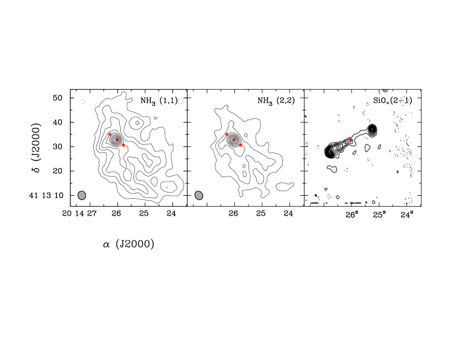
Figure 1: Images of IRAS20126 in NH₃(1,1), NH₃(2,2), and SiO(2-1). The red stars in the NH₃ images show the locations of the NH₃ spectra in figures 2 and 3. See text for absolute coordinates. The single star in the SiO image corresponds to the middle star in the other images. The angular resolution (FWHM) is indicated by the shaded ellipse, lower-left corner of each panel. The contour interval and first contour is 35 mJy kms^-1 for the NH₃(1,1) and NH₃(2,2) emission, and 130 mJy kms^-1 for the SiO(2-1). The SiO image is from Cesaroni et al. (1999).

The VLA data were processed using the NRAO Astronomical Image Processing System (AIPS) package. Data from the two days were combined to achieve an rms of 3 mJy per 0.3 km s^-1 channel for the NH₃ (1,1), (2,2) lines and 6 mJy and 4 mJy per 0.6 km s^-1 channel for the NH₃ (3,3) and (4,4) lines respectively. Figure 1 shows two images of IRAS20126 in the integrated intensity of NH₃(1,1) and (2,2). The protostar is located within the bright core of the larger scale cloud. Also shown in figure 1 is the image of the bipolar outflow in SiO(2-1) from Cesaroni et al. (1999). The NH₃ spectra used in the analysis are taken at positions offset from the phase center by -0.23, 1.00 (center), -3.10, 3.25 (left), and 2.50,-0.94 (right) in arc seconds of RA and dec. The corresponding absolute positions are R.A. (J2000) = 20:14:26.02, decl. (J2000) = 41:13:32.8 (center) , R.A. (J2000) = 20:14:25.79, decl. (J2000) = 41:13:30.8 (right) , and R.A. (J2000) = 20:14:26.28, decl. (J2000) = 41:13:35.0 (left) , The locations of the spectra are shown as red stars on figure 1.

2.2 Methyl Cyanide and Carbon Sulfide lines

The CH₃CN(13-12) observations were made with the SMA on July 10, 2006 with a maximum baseline of $\sim 0.5$ km, a beam size of $0.40\times 0.36$”, and a phase center of R.A. (J2000) = 20:14:26.02, decl. (J2000) = 41:13:32.7. The channel width is 0.8 kms^-1 at the observing frequency of 239 GHz. The rms noise of the data is 0.05 Jy beam^-1 channel^-1 or 8 K channel^-1 in brightness temperature.

Data in the CH₃CN J = 12-11, and C³⁴S J = 5-4 and J = 2-1 transitions were obtained from the IRAM interferometer between 1996 December through 1997 March, and 2002 January through March. The phase center of the observations is R.A. (J2000) = 20:14:26.03, decl. (J2000) = 41:13:32.7. The primary beam of the array at the frequency of the observed CH₃CN transitions (230 GHz) and C³⁴S(5-4) (241 GHz) is approximately $20^{\prime\prime}$ with a spatial resolution of about $0.8^{\prime\prime}$. At the lower frequency of the C³⁴S(2-1) transtion (96 GHz) the primary beam is about $50^{\prime\prime}$ and the spatial resolution is and $2.4^{\prime\prime}$. The full details of these observations can be found in Cesaroni et al. (1999, 2005).

3 The Standard Model for Star Forming Accretion Flows

3.1 The density of the accretion flow

The standard model for a star-forming accretion flow consists of an inflowing envelope around a rotationally supported disk. Similar to the approach in Whitney et al. (2003), we use the model of Ulrich (1976) to describe the gas density in the infalling envelope and standard thin-disk theory (Pringle, 1981) to describe the disk,

The model for the envelope assumes that the gas flows toward a gravitational point source along ballistic trajectories. The flow conserves angular momentum and ignores the pressure and self-gravity of the gas. This is the same envelope model that Whitney et al. (2003) adopted for low-mass stars and similar to the model used to describe the accretion flow onto a cluster of high-mass stars, G10.6-0.07 (Keto, 1990; Keto & Wood, 2006). Thus despite, or perhaps because of, its simplicity, the model has found application to accretion flows from low-mass stars to star clusters. The model is particularly useful in analyzing observational data because only 3 parameters are required to describe individual cases: 1) the density of the gas at a single radius (the gas density elsewhere follows from mass conservation), 2) the mass of the point source, and 3) the specific angular momentum.

The model for the envelope is fully described in Ulrich (1976). We use the equations as presented in Keto (2007), and Mendoza, Canto, Raga (2004). The envelope density is (equation 10 of Keto (2007)),

$$\rho_{\rm env}=\rho_{e0}(r/R_{d})^{-3/2}\bigg{(}1+{{\cos{\theta}}\over{\cos{\theta_{0}}}}\bigg{)}^{-1/2}$$

$$\quad\quad\quad\times\quad(1+(r/R_{d})^{-1}(3\cos^{2}{\theta_{0}}-1))^{-1}$$ (1)

where $\rho_{e0}=\rho_{\rm env}(R_{d})$ is the density in the mid-plane, $\theta=\pi/2$, at radius, $R_{d}$, $\theta_{0}$ is the initial polar angle of the streamline, and $\theta$ and $r$ are the polar angle and radius at each point along a streamline. The angle, $\theta$ is related to the polar radius, $r$, and the initial angle $\theta_{0}$ (equation 7 of Keto (2007)),

$$r={R_{d}\cos{\theta_{0}}\sin^{2}{\theta_{0}}\over{\cos{\theta_{0}}-\cos{\theta}}}$$ (2)

The density is related to the mass accretion rate (equation 11 of Keto (2007))

$$\dot{M}=\rho_{e0}(R_{d})4\pi R_{d}^{2}v_{k}$$ (3)

where $v_{k}$ is the Keplerian velocity at $R_{d}$.

The model for the disk assumes that a rotationally-supported disk forms at the radius where the centrifugal force in the rotating envelope equals the gravitational force of the point mass,

$${{\Gamma^{2}}\over{R^{3}_{d}}}={{GM_{\ast}}\over{R^{2}_{d}}}$$ (4)

and $\Gamma=v_{\phi}R$. The disk is truncated at $R_{d}$.

The gas density in the disk is (equation 3.14 of Pringle (1981)),

$$\rho_{\rm disk}(z,R)=\rho_{0}(R)\exp(-z^{2}/2H^{2})$$ (5)

where $\rho_{0}(R)$ is the density in the mid-plane, $\theta=\pi/2$, at any radius $R$. We use $R=\sqrt{x^{2}+y^{2}}$ to denote the cylindrical radius, and $r=\sqrt{x^{2}+y^{2}+z^{2}}$ for the polar radius. In the thin disk theory, the scale height, $H$, is

$$H^{2}=c_{s}^{2}R^{3}/GM_{\ast}$$ (6)

where $c_{s}$ is the sound speed. We follow Whitney et al. (2003) and use a modified version of this equation,

$$H=H_{0}(R/R_{\ast})^{1.25}$$ (7)

with $H_{0}=0.01R_{\ast}$. The density in the mid-plane of the accretion disk, $\rho_{0}(R)$, is

$$\rho_{0}=\rho_{d0}({{R_{d}}/{R}})^{2.25}$$ (8)

where $\rho_{d0}$ is the density in the mid-plane at $R_{d}$. Again following Whitney et al. (2003), we use an exponent of 2.25 in equation 8 rather than 2 which is derived in the thin-disk theory. As explained in Whitney et al. (2003) the modifications to the equations for the scale height and mid-plane densities are based on fits to numerical models of disk structure.

The densities in the disk and envelope at radius $R_{d}$ are related by a factor, $A_{\rho}$,

$$\rho_{d0}=A_{\rho}\rho_{e0}$$ (9)

For example, in the steady-state flow, the disk would have a higher density if, as should be the case, the inward velocities in the rotationally-supported disk were lower than in the freely-falling envelope. Because the inward velocities in the disk are not described by the thin-disk theory, we leave $A_{\rho}$ as an adjustable parameter. The total gas density at any point in the model is the sum of the densities in the disk and envelope,

$$\rho_{\rm gas}=\rho_{\rm disk}+\rho_{\rm env}$$ (10)

3.2 The temperature

We assume that the envelope is heated by the star. The envelope temperature is (equation 7.36 of Lamers & Cassinelli (1999))

$$T_{\rm env}=T_{\ast}(R_{\ast}/2r)^{2/(4+p)}$$ (11)

where $p$ in our model is an adjustable parameter related to the dust opacity and the geometry of the flow. If the density structure were spherically symmetric, then $p$ would be the exponent in the frequency dependence, $\nu^{p}$, of the Planck mean opacity of the dust. In a flattened flow, $p$ can be negative if the geometrical dilution of the radiation in the accretion flow is greater than $r^{-2}$. This can happen if the dust at each radius absorbs and isotropically re-emits the outward flowing radiation. Radiation that is emitted perpendicular to the disk escapes from the flow. Only the radiation that is emitted in the direction along the flattened flow continues to heat the dust at larger radii. The result is a decrease in the radiation in the disk faster than $r^{-2}$.

In the thin-disk theory, the disk is heated by dissipation related to the accretion rate. The disk temperature is (equation 3.23 of Pringle (1981))

$$T_{\rm disk}=B_{T}\bigg{[}\bigg{(}{{3GM_{\ast}\dot{M}}\over{4\pi R^{3}\sigma}}\bigg{)}\bigg{(}1-\sqrt{{{R_{\ast}}\over{R}}}\bigg{)}\bigg{]}^{1/4}$$ (12)

We include an adjustable factor, $B_{T}$, to allow for additional, or possibly less, disk heating. For example, the observations constrain the gas density through the observed optical depth of NH₃. This means that the density and therefore the accretion rate, $\dot{M}$, are dependent on the assumed NH₃ abundance which is not well known. The adjustable factor, $B_{T}$, decouples the disk temperature from the assumed molecular abundance. Also the disk temperature may be raised by stellar radiation (passive heating). The factor, $B_{T}$, allows for these effects in an approximate way.

The gas temperature in the model is the density weighted average of the envelope and disk temperatures,

$$T_{\rm gas}={{T_{\rm disk}\rho_{\rm disk}+T_{\rm env}\rho_{\rm env}}\over{\rho_{\rm disk}+\rho_{\rm env}}}$$ (13)

3.3 The velocity

The 3 components of the gas velocity in the envelope are given in spherical coordinates by equations 4,5,6 of Keto (2007), but there are errors in earlier papers. In particular, equations 5 and 6 of Keto (2007) and equation 8 of Ulrich (1976) are incorrect. Equation 8 of Ulrich (1976) (same as equation 5 of Keto (2007)) does not result in energy conservation, $mv^{2}/2=GM/r$, when combined with the other velocity components. The error is small, 1 part in $10^{4}$. The following equations, same as in Mendoza, Canto, Raga (2004), are exact.

$$v_{r}(r,\theta)=-\bigg{(}{{GM_{\ast}}\over{r}}\bigg{)}^{1/2}\bigg{(}1+{{\cos{\theta}}\over{\cos{\theta_{0}}}}\bigg{)}^{1/2}$$ (14)

$$v_{\theta}(r,\theta)=\bigg{(}{{GM_{\ast}}\over{r}}\bigg{)}^{1/2}\bigg{(}{{\cos{\theta_{0}}-\cos{\theta}}\over{\sin\theta}}\bigg{)}\bigg{(}1+{{\cos\theta}\over{\cos{\theta_{0}}}}\bigg{)}^{1/2}$$ (15)

$$v_{\phi}(r,\theta)=\bigg{(}{{GM_{\ast}}\over{r}}\bigg{)}^{1/2}{\sin{\theta_{0}}\over{\sin{\theta}}}\bigg{(}1-{{\cos{\theta}}\over{\cos{\theta_{0}}}}\bigg{)}^{1/2}$$ (16)

The velocity in the disk is simply the Keplerian velocity,

$$v_{\rm disk}(R)=\sqrt{GM_{\ast}/R}$$ (17)

where the velocity in the disk is purely azimuthal. We assume that the radial velocity in the rotationally-supported disk is comparatively small. The gas velocity in the model is the density weighted average of the envelope and disk velocities,

$$\vec{v}_{\rm gas}={{\vec{v}_{\rm disk}\rho_{\rm disk}+\vec{v}_{\rm env}\rho_{\rm env}}\over{\rho_{\rm disk}+\rho_{\rm env}}}$$ (18)

where $\vec{v}_{\rm env}$ is given by equations 14 through 16 and $\vec{v}_{\rm disk}$ is given by 17.

3.4 The density singularities in the accretion model

The density in the Ulrich model is singular in the mid-plane of the disk at the centrifugal radius and also at the origin. These singularities are caused by the convergence of the streamlines in the simple mathematical description of the flow. This convergence is not expected on physical grounds because gas pressure, neglected in the Ulrich model, would prevent it. We handle the singularities in two ways. We define the computational grid to have an even number of cells so that the centers of the middle cells are above and below the midplane and around the origin. Second, we smooth the density in the radial direction with a Gaussian with a width of $R_{d}/2$.

3.5 The model parameters

Based on the analyses of the previous observations cited in the introduction, we assume that the disk-envelope is viewed edge-on. The model contains 6 adjustable parameters: 1) $\rho_{0}$ sets the density of the envelope (equation 1) and the mass accretion rate (equation 3), 2) $p$ sets the exponent of the power law decrease of the temperature in the envelope (equation 11), 3) $\Gamma=v_{\phi}r$ is the specific angular momentum (equation 4) of the envelope flow, 4) $M_{\ast}$ is the stellar mass 5) $A_{\rho}$ sets the ratio (equation 9) of the disk density to the envelope density at $R_{d}$, 6) $B_{T}$ is factor multiplying the disk temperature (equation 12).

4 Fitting the model to the NH₃ data

The disk enters into the model additively, and we can test for the presence of a disk by fitting models to the data with and without the disk. In the first case, with the disk, we adjust all 6 model parameters for both the envelope and the disk, and in the second case, without the disk, we adjust only the first 4 parameters for the envelope. The fitting is done independently in each case, and the 4 envelope parameters are therefore different in the 2 cases. The procedure for fitting the data is the same as described in Keto et al. (2004). We use a fast simulated annealing algorithm to adjust the model parameters to minimize the summed squared difference ($\chi^{2}$) between the data and the model spectra.

The model spectra for each particular set of model parameters are generated by our radiative transfer code MOLLIE (Keto, 1990; Keto et al., 2004). We assume LTE conditions for the NH₃ and CH₃CN lines. The LTE approximation is appropriate for NH₃ because in the absence of strong infrared radiation the level populations are expected to be mostly in the ”metastable” states which are the lowest J-state of each K-ladder. Since radiative transitions between K-ladders are forbidden, the coupling between the metastable states is purely collisional and the population approximates a Boltzmann distribution as in LTE (Ho & Townes, 1983). CH₃CN is also a symmetric top and transitions across the K-ladders are similarly forbidden; however, unlike NH₃, the upper states are easily populated in warm gas ($>100$ K). While the justification for the LTE approximation is not as strong for CH₃CN as for NH₃, we find that CH₃CN always traces hot, very dense gas where collisional transitions should be important. For C³⁴S we use the accelerated lambda iteration algorithm (ALI) of Rybicki & Hummer (1991) to solve for the non-LTE level populations.

In comparing the model to the data, we take into account the spatial averaging of the brightness by the width of the observing beam. We compute spectra over a grid of positions and smooth the result by convolution with a Gaussian with the FWHM equivalent to the observing beam of each observation, §2.

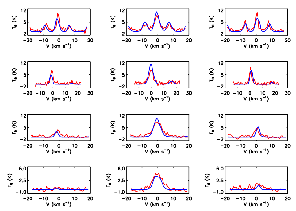
Figure 2: Data (red) and model (blue) spectra of NH₃(1,1) (top row) NH₃(2,2) (2nd row) NH₃(3,3) (3rd row) and NH₃(4,4) (bottom row) at 3 positions across the mid-plane of IRAS20126 for the accretion flow including both an infalling envelope and a flared disk. The spectra in the middle column are toward the center of the flow, and the the columns to the left and right show spectra on either side of the center, 6200 AU to the left, and 5700 au to the right. The 3 locations are shown in figure 1.

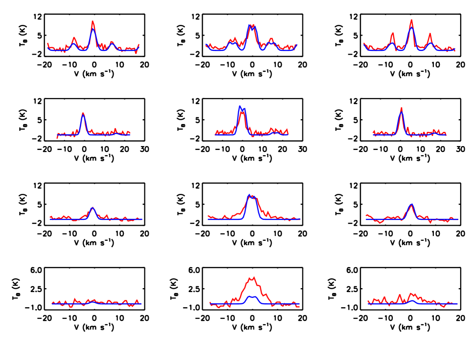
Figure 3: Spectra in the same format as figure 2 for the accretion flow with an envelope only without a flared disk.

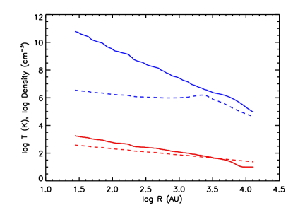
Figure 4: The temperature (red) and density (blue) for the model with both an envelope and flared disk (solid line) and for the model without a disk (dashed line). The temperatures are about the same in both models, but the disk adds considerable density. The increase in density in the envelope-only model (dashed) at 3300 AU is the smoothed density singularity at $R_{d}$ in the Ulrich (1976) model.

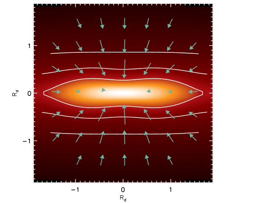
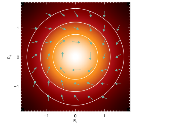
Figure 5: Density (color) and velocities (arrows) for the model with both an envelope and flared disk. Left: The XZ plane (perpendicular to the rotation) and right: the XY plane (the mid-plane of the disk and rotationally-flattened envelope). In the left panel, the color scale is logarithmic between $9.2\times 10^{4}$ and $3.7\times 10^{6}$ cm^-3. Contours (white) indicate the density at 0.006, 0.01, and 0.03, of the peak density. The longest arrow corresponds to 2.5 kms^-1 In the right panel the color scale is logarithmic between $1.1\times 10^{5}$ and $8.1\times 10^{7}$ cm^-3. Contours (white) show the density at 0.03, 0.10, and 0.3 of the peak density. The linear scale in both panels is $R_{d}=6900$ AU.

We simultaneously fit 12 NH₃ spectra, 4 transitions at 3 locations. The 3 locations are marked on figure 1. We ran twenty thousand trial models for each of the two cases with and without the disk. The spectra of the 2 best-fit models (with and without the disk) are shown in figures 2 and 3. Parameters for both cases are listed in table 1. Figure 4 shows the temperature and density in the mid-plane of our best fitting models. Figure 5 shows the density and velocity of the disk-envelope model on planes parallel and perpendicular to the rotation.

We also have CH₃CN and C³⁴S data from the observations of Cesaroni et al. (1999). The way the radiative transfer simulation program operates, we cannot use our automated search algorithm on more than one molecule at a time. The program is recompiled for each molecule. We also have not implemented the automated search for CH₃CN. We could fit the model to the C³⁴S data, but this line does not have the hyperfine structure of NH₃ that is so useful in constraining the optical depth and temperature. Therefore we opted for a different strategy. We do not use the CH₃CN or the C³⁴S data in the fitting. We use the data on these other lines as a check on the model derived from the NH₃ data. We simulate the CH₃CN and C³⁴S emission using the same two models (with and without the disk) previously derived from the NH₃ observations for comparison with the predicted spectra against the data. The models derived from the NH₃ fitting fix the temperature, densities, and velocities, but we still need to assume abundances for CH₃CN and C³⁴S. For CH₃CN we assume an abundance of $6\times 10^{-8}$. The assumed abundance of C³⁴S is $9.0\times 10^{-11}$, chosen to match the brightness of the (2-1) line.

4.1 Comparison of the model with the observed spectra

The comparison of figures 2 and 3 shows that the higher temperature and density disk and the lower temperature and density envelope are both required to fit both the high-excitation and low-excitation NH₃ spectra. Without the disk, there is not enough warm, dense gas to reproduce the (4,4) line brightness. Without the large-scale envelope, there is not enough cold gas to fit the observed ratios of the NH₃(1,1) hyperfine lines.

Further evidence for the disk component comes from the CH₃CN spectrum. The results again show that the warm, high-density, disk component is required to get enough brightness in lower frequency (higher velocity) K transitions. Based on the observed line width, the CH₃CN(12-11) emission comes from gas very close to the star. The observed CH₃CN(12-11) lines that are not blended with other molecular lines, have line widths of 10.0 kms^-1. The 2 lines that appear much broader in the data contain contaminating emission from transitions of CH¹³CN(12-11) and HNCO (Cesaroni et al., 1999). Rotational velocities $>10$ kms^-1 are only found at radii closer than 600 AU ($<GM/v^{2}$) around a 10 M_⊙ star. Figure 4 shows that the gas in the disk has a temperature of greater than 150 K within this radius. Thus the CH₃CN emission derives mostly from warm gas that is very close to the star and is thus a good molecular tracer of the inner disk.

The CH₃CN(13-12) spectra is too noisy to help discriminate between the two cases. The peak signal-to-noise ratio is about 6 after smoothing by every other channel. Nonetheless, the models are at least consistent with these observations.

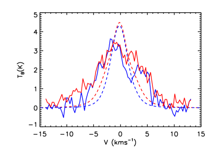
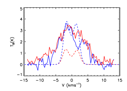
Figure 7: C³⁴S(2-1) (blue) and C³⁴S(5-4)(red) spectra of the data (solid lines) and the model (dashed lines). Left: Model with both the accretion envelope and flared disk. Right: Model with only an accretion envelope and without a flared disk. The brightness of the C³⁴S(5-4) spectra, both observed and modeled, have been divided by 6. The comparison shows that the model with the disk produces the correct brightness ratio. Without the disk, the C³⁴S(5-4) line is not bright enough and both lines have the wrong profile shape. The zero velocity refers to the model. The observed spectra have been shifted to match.

The brightness ratio of the C³⁴S (5-4) and (2-1) lines also suggests the presence of a warm, dense disk (figure 7). The model with the disk reproduces the observed brightness ratio, 6:1 for the 2 lines, although line width is less than observed. The model without the disk is not able to generate sufficient brightness in the higher excitation line, and the shapes of the line profiles do not match the data. In particular, the strong splitting that is seen in the model profiles without the disk is not seen in the data. This difference is also seen in the NH₃ and CH₃CN spectra of the 2 models, although not as prominently. We usually associate split line profiles with spatially unresolved observations of Keplerian disks (Beckwith & Sargent, 1993) whereas here the disk produces a triangular profile. What happens here is that the disk component is spatially resolved and has a very high density. Thus within the beam through the center of the model there is a lot of high density gas from the outer part of the disk with very low velocity projected along the line-of-sight. This gas disk creates the peak in the spectrum around zero velocity. In the envelope-only model without the high density disk, the model is optically thin in C³⁴S. In this case, we get the usual split line profiles from the rotation and infall in the envelope.

4.2 Goodness of fit

How well do the data constrain the model parameters? Some appreciation can be gained by plotting $\chi^{2}$ obtained from all the trial models versus each model parameter. Each panel shows the fits obtained (ordinate) for each value of a single parameter (abscissa) as all the other parameters are varied. The lowest value of $\chi^{2}$ (ordinate) at each parameter value (abscissa) is the best fit that can be obtained for that parameter value, for any combination of all the other parameters. The formal error of a model parameter is proportional to the second derivative of $\chi^{2}$ with respect to the model parameter. Thus the curvature or width of the lower boundary of the collection of points in each figure is a qualitative measure of the sensitivity of the model to the parameter.

5 Discussion

5.1 The density

The gas density is constrained by the optical depths of the NH₃ lines, which can be determined from the brightness ratios of the hyperfine lines. The density, $\rho_{0}$, at $R_{d}$ is $7.9\times 10^{4}$ (table 1) assuming an NH₃ abundance of $10^{-7}$. With this abundance, the mass of the disk is 2.5 M_⊙, the mass of the envelope is 12.6 M_⊙, and the accretion rate (equation 3), asssumed to be the same in the envelope and the disk, is $\dot{M}=7.6\times 10^{-5}$ M_⊙ yr^-1. The total mass in the accretion flow is mass of the disk and envelope together which is 15.1 M_⊙. This mass estimate is the total mass within the model boundary of 26000 AU. Cesaroni et al. (1999) estimates that there is between 0.6 and 8.0 M_⊙ within a radius of 5000 AU.

The mass estimate derived from molecular line observations is subject to a large uncertainty. The radiative transfer modeling determines the column density of NH₃ rather than H₂. Therefore, the gas density, the masses of the disk and envelope, and the accretion rate depend inversely on the assumed abundance of NH₃ which is not well known. Estimates from models and observations of similar clouds range from $10^{-9}$ to $10^{-6}$ (Herbst & Klemperer, 2003; Keto, 1990; Estalella et al., 1993; Caproni et al., 2000; Galvan-Madrid et al., 2009). Thus the abundance of NH₃ may be uncertain by more than an order of magnitude, yet a factor of 2 in the masses of the disk and envelope is significant in an interpretation of the accretion dynamics. Furthermore, the abundance of NH₃ could be different in the disk and envelope. Estimates of the NH₃ abundance are generally lowest in colder clouds and highest in warm gas around massive stars. Some NH₃ may be frozen onto dust grains in colder gas and sublimated into the gas phase as the temperature rises. Therefore, it is possible that the NH₃ abundance is higher in the warm disk than the cold envelope. If so, the mass of the envelope could be higher than 12.6 M_⊙, assuming a lower abundance, without necessarily implying a higher mass for the disk.

5.2 The disk density factor

In the model with the flared disk, the density in the mid-plane of the disk at the radius of the disk boundary $R_{d}$ is 5 times more dense than the smoothed density of the envelope at the same point. Considering that the gas density changes by 6 orders of magnitude across the model, there is little discontinuity between the envelope and disk densities (figure 4). In the model without the disk the smoothed density is approximately constant from $R_{d}$ to the origin (figure 4).

5.3 The stellar mass

The stellar mass, 10.7 M_⊙, is constrained primarily by the disk velocities (equation 17 ) required to match the observed linewidths (about 10 kms^-1) and the gas temperature that determines the brightness ratios of the low and high excitation lines. The gas velocities and therefore line widths due to unresolved motions within the beam depend on the stellar mass because the velocities are proportional to the square root of the mass. The gas temperature depends on the mass of the star because the stellar temperature is a strong function of the stellar mass and because the accretion rate depends on the stellar mass. In the disk, heating by both the star and by accretion (dissipation) are important (equations 11, 12 and 13 ). In the best-fit model, the disk temperature would be about 1/3 lower without the passive heating from the star, The temperature of the infalling envelope is determined entirely by the stellar temperature (equation 11).

5.4 The angular momentum of the envelope

The angular momentum of the envelope is determined from the widths of the spectral lines and from the VLSR of the NH₃ spectra at the locations left and right of the center. If there were too much rotation then both of the off-center spectra would have an incorrect V_LSR; too little, and all the NH₃ line widths would be too narrow. The disk radius, $R_{d}=6900$, is set by the angular momentum in the envelope, $\Gamma$, and the stellar mass (equation 4). The velocity at $R_{d}$, $v_{k}=1.2$ kms^-1, increases inward as $R^{-1/2}$. We assume a microturbulent broadening of 1 kms^-1, added in quadrature to the thermal broadening. Since the observed line widths are about 10 kms^-1 most of the width of the spectral lines comes from rotation and infall in the model.

The model radius of 6900 AU seems large, and we would regard this as an upper limit. First, the Ulrich flow conserves angular momentum whereas real accretion flows probably involve some braking of the spin-up. If the spin-up were slower, then the disk would be found at a smaller radius. Second, the high density of the disk is helpful in providing optical depth to strengthen the NH₃(1,1) outer hyperfines. The Ulrich flow has a density singularity in the mid-plane which we have handled as desribed in §3.4 by a combination of gridding and smoothing. Maybe our mid-plane density in the envelope is too low, and to compensate, the thin disk is bigger.

5.5 The exponent of the temperature power law

The modelling suggests that the temperature of the envelope falls off very quickly away from the star, as $r^{-1}$. This implies that the dilution of the radiation is faster than spherical, $r^{-2}$. The rapid dilution is consistent with the rotationally flattened geometry. At each radius, radiation is absorbed and re-emitted by dust in the flow. In a flattened flow, much of this reprocessed radiation escapes vertically out of the flow. In contrast, in a spherical flow, all the reprocessed radiation continues to interact with the flow at larger radii. If the gas temperature decreases outward fast enough that most of the envelope is at the minimum gas temperature, then a larger value of the exponent (more negative value of the parameter $p$ in equation 11) would have no further effect. We assume a minimum temperature of 10 K, a typical temperature of molecular gas, We derive an upper limit $p<-1$.

5.6 The disk temperature multiplier

The disk temperature multiplier determines the relative importance of active disk heating, owing to accretion and dissipation (equation 12), and passive heating from the protostar (equation 11). With active disk heating, the temperature in the disk is about 50% above that from passive heating alone.

6 Conclusions

This investigation shows that a standard model of a freely-falling, rotationally-flattened accretion envelope around a rotationally supported disk is able to reproduce the NH₃, CH₃CN, and C³⁴S spectral line observations of IRAS20126. Both the disk and envelope components are required to fit the observed brightness of both the low and high excitation lines, and to fit the observed line widths.

This disk-envelope model was developed for low-mass stars and is quite successful in explaining many of their observable characteristics. The success of this model in explaining the molecular line observations of the massive star IRAS20126 suggests that at least up to 10 M_⊙, the accretion processes of massive stars are similar to those of solar mass stars.

There are some differences. Although the mass of the disk is uncertain owing to its dependence on the NH₃ abundance, the disk mass is a significant fraction of the mass of the star. Furthermore, the extent of the disk is quite large, $\sim$6900 AU. This suggests that self-gravity in the disk is dynamically important, and therefore, the disk may be unstable to local fragmentation and the formation of companion stars.

The physical model in combination with the molecular line radiative transfer presented in this paper has a further application to other massive star forming regions. The spatial resolution and sensitivity of the present generation of interferometers cannot spatially resolve accretion disks in massive protostellar objects at multi-kpc distances. However, spectral lines sampling a wide range of densities and temperatures can still provide constraints to the physical structure of the core and disk. As shown in IRAS20126, the spectral lines formed in the higher density and temperature regions confirm the presence of an accretion disk. While future observatories such as ALMA will be able to spatially resolve the flow on the disk scale, before the science commissioning of ALMA, this method is a promising technique to probe the spatially unresolved regions of the flow and disk using data from the current interferometers.

Table 1: Model Parameters.

Parameter	Symbol	Disk	No Disk
Env. Density at $R_{d}$ (cm-3)	$\rho_{0}$	$7.9\times 10^{4}$	$7.9\times 10^{5}$
Temperature power law exp.	$p$	$<-1$	0.4
Angular Momentum (AU kms-1)	$\Gamma$	8100	3500
Stellar Mass (M⊙)	M∗	10.7	7.3
Disk Density Ratio	$A_{\rho}$	5.1	…
Disk Temperature factor	$B_{T}$	15.0	…
Centrifugal radius (AU)	$R_{d}$	6900	1900
Velocity at $R_{d}$ (kms-1)	$v_{k}$	1.2	1.8
Total mass1 within 0.128 pc ($M_{\odot}$)		12.6	10.1
Disk mass ($M_{\odot}$)		2.5	…
Envelope accretion rate ($M_{\odot}$ yr-1)		$7.6\times 10^{-5}$	$1.0\times 10^{-4}$
1 The mass estimates include the envelope and the disk for the case
with a disk, and the envelope only for no disk.
Both cases assume an NH3 abundance of $1.0\times 10^{-7}$.

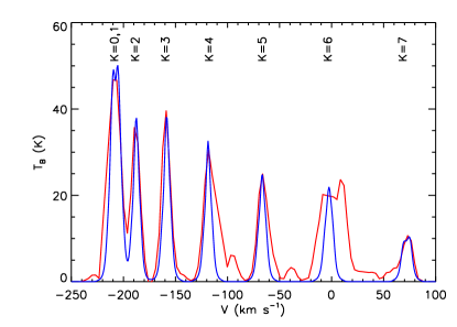
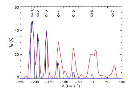
Figure 6: Data (red) and model (blue) spectra of CH₃CN(12-11). The left panel shows the spectrum for the model with both an accretion envelope and flared disk. The model is the same as shown in figures 2, 4, 5. The right panel is for the model with only an accretion envelope and without a disk (figures 3, 4). In the observed spectrum, the line that is anomalously wide (K=6, 2nd from right) is contaminated by HNCO emission. Additionally, contamination from weak CH${}_{3}^{13}$CN emission shows up to the red (right) of 4 of the lines. The velocity of the K=6 hyperfine line has been set to zero. The observed spectra have been shifted in velocity to match.

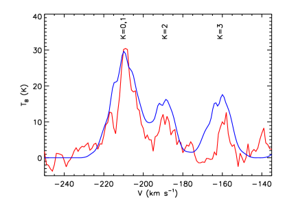
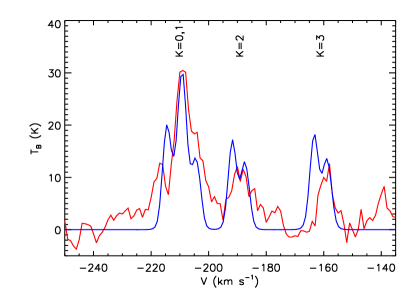
Figure 8: Spectra of CH₃CN(13-12) in the same format as figure 6 except that we have only the 4 lowest K transitions. The K=0 and K=1 transitions are blended together in the bluest peak. The left panel shows the spectrum for the model with both an accretion envelope and flared disk. The right panel is for the model with only an accretion envelope and without a disk (figures 3, 4). The signal-to-noise ratio of the observed spectra, about 6 at the peak, is not high enough to discriminate between the two models. At least the models are consistent with the data. The data are from T.K. Sridharan (private communication).

Figure 9: The value of $\chi^{2}$ as a function of a single parameter. The plots show $\chi^{2}$ for the better fitting disk-envelope models as a function of a single parameter. The width of the collection of points in each figure is a qualitative measure of the sensitivity of the models to each parameter. Values of the parameters outside the range shown by the lower $\chi^{2}$ values produce very poor fits. The units of the density are the log of $cm^{-3}$, the units of stellar mass are $M_{\odot}$, and the units of angular momentum are AU $\times$ kms^-1 divided by 1000. The parameters are listed in Table 1.

References

- Andre et al. (1993) Andre, P., Ward-Thompson, D., & Barsony, M., 1993, 406, 122
- Caproni et al. (2000) Caproni, A., Abraham, Z., & Vilas-Boas, J.W.S., 2000, AA, 361, 685
- Cesaroni et al. (1997) Cesaroni, R., Felli, M., Walmsley, C.M., & Olmi, L, 1997, AA, 325, 725
- Cesaroni et al. (1999) Cesaroni, R., Felli, M., Jenness, T., Neri, R., Olmi, L., Robberto, M., Testi, L., Walmsley, C.M., 1999, AA, 345, 949
- Cesaroni et al. (2005) Cesaroni, R., Neri, R., Olmi, L., Testi, L., Walmsley, C.M., & Hofner, P., 2005, AA, 434, 1039
- Estalella et al. (1993) Estalella, R., Mauersberger, R., Torrelles, J.M., Anglada, G., Gomez, J.F., Lopez, R., Murders, D., 1993, ApJ, 419,698
- deBuizer (2007) deBuizer J.M., 2007, ApJ, 654, L147
- Galvan-Madrid et al. (2009) Galvan-Madrid, R., Keto, E., Zhang, Q., Kurtz, S., Rodriguez,L.F., Ho, P.T.P., 2009, ApJ, submitted
- Herbst & Klemperer (2003) Herbst, E. & Klemperer, W., 1973, ApJ, 616, 301
- Keto, Ho & Haschick (1987) Keto, E., Ho, P., & Haschick, A., 1987, ApJ, 318, 712
- Cesaroni et al. (1994) Cesaroni, R., Churchwell, E., Hofner, P., Walmsley, C.M., & Kurtz, S., 1994, AA, 288, 903
- Hartmann (2001) Hartmann, L., Accretion Processes in Star Formation Cambridge, UK: Cambridge University Press
- Ho & Townes (1983) Ho, P.T.P., Townes, C.H., 1983, ARAA, 21, 239
- Kahn (1974) Kahn, F.D., 1974, AA, 37, 149
- Kawamura et al. (1999) Kawamura, J.H., Hunter, T.R. , Tong, C.-Y.E., Blundell, R., Zhang, Q., Katz, C., Papa, D.C. & T.K. Sridharan, 1999, PASP, 111, 1088
- Keto (1990) Keto, E., 1990, ApJ, 355, 190
- Keto (2002) Keto, E. 2002b, ApJ, 580, 980
- Keto et al. (2004) Keto, E., Rybicki, G.B., Bergin, E.A., Plume, R., 2004, ApJ, 613, 355
- Keto & Wood (2006) Keto, E. & Wood, K., 2006, ApJ, 637, 850
- Keto (2007) Keto, E., 2007, ApJ, 666, 976
- Kumar & Grave (2007) Kumar M.S.N. & Grave, J.M.C., 2007, AA, 472, 155
- Lada (1987) Lada, C.J., in IAU Symp. 115, Star Forming Regions, ed. M Peimbert & J.Jugaku (Dordrecht:Kluwer), 1
- Lamers & Cassinelli (1999) Lamers, H.J.G.L.M. & Cassinelli, J.P., 1999, Introduction to Stellar Winds Cambridge, UK: Cambridge University Press
- Larson & Starrfield (1971) Larson, R.B. & Starrfield, S., 1971, AA, 13, 190
- Lebron et al. (2006) Lebron, M., Beuther, H., Schilke, P. & Stanke, T. 2006, AA, 448, 1037
- Mendoza, Canto, Raga (2004) Mendoza, S., Canto, J., Raga, A.C., 2004 Rev. Mex. AA, 40, 147
- Pringle (1981) Pringle J., 1981, ARAA, 19, 137
- Qiu et al. (2008) Qiu, Keping, Zhang, Qizhou, Megeath, S Thomas, Gutermuth, Robert A., Beuther, Henrik, Shepherd, Debra S., Testi, L., and De Pree, C. G. 2008, ApJ, 685, 1005
- Rybicki & Hummer (1991) Rybicki, G.B. & Hummer, D.G., 1991, AA, 245, 171
- Beckwith & Sargent (1993) Beckwith, S.V.W. & Sargent, A.I., 1993, ApJ, 402, 280
- Shepherd et al. (2000) Shepherd, D. S., Yu, K. C., Bally, J. & Testi, L. 2000, ApJ, 535, 833
- Shu, Adams, Lizano (1987) Shu, F.H., Adams, F.C., Lizano, S., 1987, ARAA, 25, 23
- Sridharan, Williams, & Fuller (2005) Sridharan, T.K., Williams, S.J., & Fuller, G.A., 2005, ApJ, L73
- Su et al. (2007) Su, Yu-Nung, Liu, Sheng-Yuan, Chen, Huei-Ru, Zhang, Qizhou, and Cesaroni, Riccardo, 2007, ApJ, 671, 571
- Ulrich (1976) Ulrich J., 1976, ApJ, 210, 377
- Whitney et al. (2003) Whitney, B.A., Wood, K., Bjorkman, J.E., Wolff, M.J., 2003, ApJ, 591, 1049
- Whitney et al. (2008) Whitney, B.A., et al., 2008, AJ, 136, 18
- Wilking, Lada, Young (2007) Wilking, Bruce A, Lada, Charles J., & Young, Eric T. 1989, ApJ, 340, 823
- Wolfile & Cassinelli (1987) Wolfire, M.G., Cassinelli, J.P., 1987, ApJ, 319, 850
- Zhang, Hunter, & Sridharan (1998) Zhang, Q., Hunter, T.R., Sridharan, T.K., 1998, ApJ, 505, L151
- Zhang et al. (1999) Zhang, Q., Hunter, T. R., Sridharan, T. K., & Cesaroni, R., 1999, Astrophysical Journal, 527, L117