Charge-density-wave formation in a half-filled fermion-boson transport model:
a projective renormalization approach

Abstract

We study the metal-insulator transition in a very general two-channel transport model, where charge carriers are coupled to a correlated background medium. The fluctuations of the background were described as bosonic excitations, having the ability to relax. Employing an analytical projector-based renormalization technique, we calculate the ground-state and spectral properties of this fermion-boson model and corroborate recent numerical results, which indicate—in dependence on the ‘stiffness’ of the background medium—a Luttinger-liquid to charge-density-wave transition for the one-dimensional half-filled band case. In particular, we determine the renormalized electron and boson dispersion relations and show that the quantum phase transition is not triggered by a softening of the boson modes. Thus the charge density wave is different in nature from an usual Peierls distorted state.

I Introduction

Charge density waves (CDWs) are broken symmetry states of metals that predominantly appear in materials which have a highly anisotropic crystal and electronic structure Grüner (1994). The formation of CDWs strongly depends on the band-filling and on the topology of the Fermi surface. Concerning the latter, one-dimensional (1D) systems are peculiar, because their Fermi surface consists of two points only. Not surprisingly, electron-electron and electron-phonon interactions, which are the driving forces behind most metal-insulator transitions, have more impact in reduced dimensions. At the same time, however, quantum fluctuations and finite-temperature effects—both counteracting any development of long-range order—become increasingly important as well. Then, all in all, in 1D, usually a rather complex interplay between the charge, spin, orbital and lattice degrees of freedom evolves, which, of course, will strongly affect the transport properties of the system. Prominent examples are quasi-1D halogen-bridged transition metal complexes (MX-chains) Bishop and Swanson (1993).

The theoretical description of such highly correlated 1D systems is frequently based on ‘microscopic’ models like the half-filled SSH Su et al. (1979), Holstein Holstein (1959); Bursill et al. (1998); Hohenadler et al. (2006), Peierls Peierls (1955), Hubbard Hubbard (1963), (quarter-filled) $t$-$J$ models Mutou et al. (1998), or combination of these Takada and Chatterjee (2003). Thereby, the complexity of the electron-electron or electron-phonon interactions in the Hamiltonians usually prevents the exact (numerical) solution of the model in the thermodynamic limit, which would be necessary in order to pinpoint a true quantum phase transition between a metal and a CDW.

To some extent, the state of affairs improves if one considers simplified transport models instead, where particle motion takes place in an effective background medium. The ‘background’ reflects the correlations inherent in the system, e.g., the charge-, orbital- or spin-order in a solid. That quasiparticles move through an ordered insulator is a very general situation in condensed matter physics Wohlfeld et al. (2009); Berciu (2009). This scenario also applies to soft matter systems like DNA, where the charge transport on the backbone is affected by the ‘configuration’ of chemical side groups, which, vice versa, depends on the physical presence of charge carriers Komineas et al. (2007).

Along this line, a novel fermion-boson quantum transport model,

$$H=-t_{b}\sum_{\langle i,j\rangle}c_{j}^{\dagger}c_{i}(b_{i}^{\dagger}+b_{j})-\lambda_{b}\sum_{i}(b_{i}^{\dagger}+b_{i})+\omega_{b}\sum_{i}b_{i}^{\dagger}b_{i}\,,$$ (1)

has been proposed a few years ago Edwards (2006), and was shortly afterwards solved for a single particle ($N_{e}=1$) in a 1D infinite system Alvermann et al. (2007) by a variational numerical diagonalization technique Alvermann et al. (2007). The Hamiltonian (1) mimics the ‘background’ by bosonic degrees of freedom [$b_{i}^{(\dagger)}$], which influence and even may control the transport of fermionic particles [$c_{i}^{(\dagger)}$] on the $N$ sites of a regular lattice. Every time a particle hops between nearest-neighbor Wannier sites $\langle i,j\rangle$, it creates (or destroys) a local excitation of energy $\omega_{b}$ in the background medium at the site it leaves (it enters). Clearly these distortions tie the particle to its origin (cf. the string effect as a hole moves in a Néel spin background). Of course, any distortion of the background can heal out by quantum fluctuations (again, one can have spin fluctuations in mind). Accordingly, in the Hamiltonian (1), the $\lambda_{b}$-term was included, allowing for spontaneous boson creation and annihilation processes.

Strong correlations, nevertheless, may evolve in a system described by the Hamiltonian (1), provided the background excitations have a rather large energy and the ability of the background medium to relax is small, i.e.,

$$\Omega=\frac{\omega_{b}}{t_{b}}\gg 1\quad\mbox{and}\quad\Lambda=\frac{\lambda_{b}}{t_{b}}\ll 1\,.$$ (2)

For the half-filled band sector ($N_{e}=N/2$), these correlations may even drive the system into an insulating state by establishing CDW long-range order. This has been shown quite recently for the 1D case: small cluster diagonalizations Wellein et al. (2008) and density matrix renormalization group (DMRG) calculations supplemented by finite-size scaling Ejima et al. (2009); Ejima and Fehske (2009) give strong evidence for a Tomonaga-Luttinger-liquid (TLL) CDW quantum phase transition as $\Lambda$ becomes small at large enough $\Omega$. These purely numerical approaches rely on an (inevitable) truncation of the bosonic Hilbert space. Determining the metal-insulator phase boundary this seems to be uncritical, because the CDW found at half-filling is a few-boson state. The situation becomes more difficult if we enter the fluctuation-dominated regime of small $\Omega$, where many bosons are excited in the system.

In the present work, we investigate the fermion-boson transport model (1) by means of an analytical approach, which avoids these disadvantages. This approach, called projective renormalization method (PRM) Hübsch et al. (2008), is based on a sequence of discrete unitary transformations, so that—in contrast to continuous (e.g. flow-equation based) unitary transformation schemes Wegner (1994)—a direct link to perturbation theory can be provided. The method has already been successively applied to a number of many-particle models Hübsch and Becker (2005); Sykora et al. (2005); Becker et al. (2007b); Hübsch et al. (2008). Here we will analyze the ground-state and spectral properties of the Hamiltonian (1) exclusively for the half-filled band case, in both the metallic and insulating regimes. In particular we study the signatures of the TLL-CDW transition in terms of the renormalized quasiparticle band and boson dispersion, and the boson spectral function. The paper is organized as follows. In Sec. II. A we briefly resume the basic concepts behind the PRM approach. The application of the PRM to the fermion-boson transport model will be described in detail in Sec. II B. Section III presents the results of the numerical evaluation of the renormalization equations. We conclude in Sec. VI.

II Theoretical approach

II.1 Projector-based renormalization method

The PRM starts from the usual decomposition of a many-particle Hamiltonian into a solvable unperturbed part $H_{0}$ and a perturbation $H_{1}$, where $H_{1}$ should not contain any part that commutes with $H_{0}$. Thus, the perturbation $H_{1}$ consists of transitions between the eigenstates of $H_{0}$ with non-vanishing transition energies. The basic idea of the PRM is to construct an effective Hamiltonian $H_{\lambda}=H_{0,\lambda}+H_{1,\lambda}$ with renormalized parts $H_{0,\lambda}$ and $H_{1,\lambda}$, where all transitions with energies $|E_{0,\lambda}^{n}-E_{0,\lambda}^{m}|$ larger than a given cutoff energy $\lambda$ are eliminated. $E_{0,\lambda}^{n}$ and $E_{0,\lambda}^{m}$ denote the eigenenergies of $H_{0,\lambda}$.

The renormalization procedure starts from the cutoff energy $\lambda=\bar{\lambda}$ of the original model $H$ and proceeds in steps of $\Delta\lambda$ to lower values of $\lambda$. Every renormalization step is performed by means of a unitary transformation,

$$H_{\lambda-\Delta\lambda}=e^{X_{\lambda,\Delta\lambda}}\,H_{\lambda}\,e^{-X_{\lambda,\Delta\lambda}}.$$ (3)

The generator $X_{\lambda,\Delta\lambda}$ of the unitary transformation has to be fixed appropriately (for details see Ref. Hübsch et al., 2008). For instance, in lowest order perturbation theory, it reads

$$X_{\lambda,\Delta\lambda} = \frac{1}{{\bf L}_{0,\lambda}}{\bf Q}_{\lambda-\Delta\lambda}{H}_{1,\lambda}\,.$$ (4)

Here, ${\bf L}_{0,\lambda}$ is the Liouville superoperator of the ‘unperturbed’ Hamiltonian ${H}_{0,\lambda}$, which is defined by the commutator of ${H}_{0,\lambda}$ with any operator variable $A$, i.e. ${\bf L}_{0,\lambda}A=[H_{0,\lambda},A]$, and ${\bf Q}_{\lambda-\Delta\lambda}$ is a projection superoperator, which projects on all transitions with respect to the eigenspectrum of ${H}_{0,\lambda-\Delta\lambda}$ with transition energies larger than $\lambda-\Delta\lambda$. In this way difference equations can be derived which connect the parameters of $H_{\lambda}$ with those of $H_{\lambda-\Delta\lambda}$, and which are called renormalization equations.

The limit $\lambda\rightarrow 0$ provides the desired effective Hamiltonian $\tilde{H}=H_{\lambda\rightarrow 0}=H_{0,\lambda\rightarrow 0}$ where the elimination of the transitions originating from the perturbation $H_{1}$ leads to a renormalization of the parameters of $\tilde{H}$. Note that $\tilde{H}$ is diagonal or at least quasi-diagonal and allows to evaluate physical quantities. The final results depend on the parameter values of the original Hamiltonian $H$. Finally, we note that $\tilde{H}$ and $H$ have the same eigenvalue problem since both Hamiltonians are connected by a unitary transformation.

To evaluate expectation values of operators $A$, formed with the full Hamiltonian, we have to apply the unitary transformation as well,

$$\langle A\rangle=\frac{{\rm Tr}Ae^{-\beta H}}{{\rm Tr}e^{-\beta H}}=\langle A(\lambda)\rangle_{H_{\lambda}}=\langle\tilde{A}\rangle_{\tilde{H}}\,,$$ (5)

where we define $A(\lambda)=e^{X_{\lambda}}Ae^{-X_{\lambda}}$ and $\tilde{A}=A(\lambda\rightarrow 0)$. Thus additional renormalization equations are required for $A(\lambda)$.

II.2 Application to the two-channel transport model

II.2.1 Renormalization equations

We first rewrite the model (1), performing a unitary transformation $b_{i}\mapsto b_{i}+\lambda_{b}/\omega_{b}$ that eliminates the boson relaxation term in favor of a free-particle hopping channel,

$$H=-t_{f}\sum_{\langle i,j\rangle}c_{j}^{\dagger}c_{i}-t_{b}\sum_{\langle i,j\rangle}\;c_{j}^{\dagger}c_{i}(b_{i}^{\dagger}+b_{j})+\omega_{b}\sum_{i}\;b_{i}^{\dagger}b_{i}\,,$$ (6)

with

$$\frac{t_{f}}{t_{b}}=2\frac{\lambda_{b}}{\omega_{b}}=2\frac{\Lambda}{\Omega}\,.$$ (7)

This makes the two transport channels contained in the Hamiltonian (1) explicit: the coherent particle transfer, which takes place on an energy scale $(\propto t_{f})$, and the boson-affected hopping $(\propto t_{b})$.

Next, in order to exploit the translation invariance, we consider the Hamiltonian (6) in momentum space

$$H = \sum_{k}\varepsilon_{k}c_{k}^{{\dagger}}c_{k}+\omega_{b}\sum_{q}b_{q}^{{\dagger}}b_{q}$$ (8)

$$+\frac{1}{\sqrt{N}}\sum_{k,q}g_{k}\big{(}b_{q}^{{\dagger}}c_{k}^{{\dagger}}c_{k+q}+b_{q}c_{k+q}^{{\dagger}}c_{k}\big{)}\,.$$

In what follows, we consider a 1D lattice with lattice constant $a$, i.e., $\varepsilon_{k}=-2t_{f}\cos{ka}$ and $g_{k}=-2t_{b}\cos{ka}$.

Going forward, it turns out to be useful to remove the mean-field part from the fermion-boson coupling term. Defining fluctuation operators,

$$\delta(c_{k}^{\dagger}c_{k+q})=c_{k}^{\dagger}c_{k+q}-\langle c_{k}^{\dagger}c_{k}\rangle\,\delta_{q,0}\,,$$ (9)

the Hamiltonian (8) takes the form

$$H = \sum_{k}\varepsilon_{k}c_{k}^{{\dagger}}c_{k}+\omega_{b}\sum_{q}b_{q}^{{\dagger}}b_{q}$$ (10)

$$+\frac{1}{\sqrt{N}}\sum_{k}g_{k}\langle c_{k}^{\dagger}c_{k}\rangle(b_{0}^{\dagger}+b_{0})$$

$$+\frac{1}{\sqrt{N}}\sum_{k,q}g_{k}\big{[}b_{q}^{{\dagger}}\delta(c_{k}^{{\dagger}}c_{k+q})+b_{q}\delta(c_{k+q}^{{\dagger}}c_{k})\big{]}\,.$$

Obviously, the purely bosonic part of $H$, i.e. the second and third term of Eq.(10), can be diagonalized by a shift of the bosonic operators. Introducing new bosonic creation operators,

$$B_{q}^{\dagger}=b_{q}^{\dagger}+\frac{1}{\sqrt{N}}\sum_{k}\frac{g_{k}}{\omega_{b}}\langle c_{k}^{\dagger}c_{k}\rangle\delta_{q,0}\,,$$ (11)

the Hamiltonian (10) can be rewritten as $H=H_{0}+H_{1}$ with

$$H_{0} = \sum_{k}\Big{(}\varepsilon_{k}-2g_{k}\frac{1}{N}\sum_{k^{\prime}}\frac{g_{k^{\prime}}}{\omega_{b}}\langle c_{k^{\prime}}^{\dagger}c_{k^{\prime}}\rangle\Big{)}\,c_{k}^{{\dagger}}c_{k}$$ (12)

$$+\omega_{b}\sum_{q}B_{q}^{{\dagger}}B_{q}+\frac{1}{N\omega_{b}}\Big{(}\sum_{k}g_{k}\langle c_{k}^{\dagger}c_{k}\rangle\Big{)}^{2},$$

$$H_{1} = \frac{1}{\sqrt{N}}\sum_{k,q}g_{k}\Big{[}B_{q}^{{\dagger}}\delta(c_{k}^{{\dagger}}c_{k+q})+B_{q}\delta(c_{k+q}^{{\dagger}}c_{k})\Big{]}.$$ (13)

Following the ideas of the PRM approach, we make the following ansatz for the renormalized Hamiltonian ${H}_{\lambda}$ (after all transitions with energies larger than $\lambda$ have been integrated out), $H_{\lambda}=H_{0,\lambda}+H_{1,\lambda}$, where

$$H_{0,\lambda} = \sum_{k}\varepsilon_{k,\lambda}c_{k}^{{\dagger}}c_{{k}}+\sum_{k}\Delta_{k,\lambda}c_{k}^{{\dagger}}c_{k+Q}$$ (14)

$$+\sum_{q}\omega_{q,\lambda}B_{q}^{{\dagger}}B_{q}+E_{\lambda}\,,$$

$$H_{1,\lambda}=\frac{1}{\sqrt{N}}\sum_{k,q}g_{k}\Theta_{k,q}(\lambda)\Big{[}B_{q}^{{\dagger}}\delta(c_{k}^{{\dagger}}c_{k+q})+B_{q}\delta(c_{k+q}^{{\dagger}}c_{k})\Big{]}\,.$$ (15)

The $\Theta$-function in (15)

$$\Theta_{k,q}(\lambda)=\Theta(\lambda-|\varepsilon_{k,\lambda}-\varepsilon_{k+q,\lambda}+\omega_{q,\lambda}|)$$

guarantees that only transitions with excitation energies smaller than $\lambda$ remain in $H_{1,\lambda}$. In $H_{0,\lambda}$, also a symmetry breaking field, $\Delta_{k,\lambda}$, was introduced which couples together particle-hole excitations with wave vectors $k$ and $k+Q$, where $Q=\pi/a$. Note that the renormalization of $\Delta_{k,\lambda}$ may lead to a transition to a CDW ground state at half filling.

By integrating out all transitions between the cutoff of the original model $\bar{\lambda}$ and $\lambda=0$, all parameters of the original model will become renormalized. To find their $\lambda$-dependence, we derive renormalization equations for the parameters $\varepsilon_{k,\lambda}$, $\Delta_{k,\lambda}$, $\omega_{q,\lambda}$, and $E_{\lambda}$. The coupling parameter $g_{k}$ is not renormalized when we restrict ourselves to lowest order perturbation theory in one renormalization step. The initial parameter values are determined by the original model ($\lambda=\bar{\lambda}$):

$$\varepsilon_{k,\bar{\lambda}} = \varepsilon_{k}-2g_{k}\frac{1}{N}\sum_{k^{\prime}}\frac{g_{k^{\prime}}}{\omega_{b}}\langle c_{k^{\prime}}^{\dagger}c_{k^{\prime}}\rangle\,,$$ (16)

$$E_{\bar{\lambda}} = \frac{1}{N\omega_{b}}\Big{(}\sum_{k}g_{k}\langle c_{k}^{\dagger}c_{k}\rangle\Big{)}^{2}\,,$$ (17)

$$\Delta_{k,\bar{\lambda}} = 0^{+}\,,\;\;\mbox{and}\;\;\;\omega_{q,\bar{\lambda}}\,=\,\omega_{b}\,.$$ (18)

Let us assume that the symmetry breaking field $\sim\Delta_{k,\lambda}$ can be considered as small compared to the hopping part in ${H}_{0,\lambda}$. In this case, the dynamics of ${H}_{0,\lambda}$ is approximately governed by

$$\,[H_{0,\lambda},c_{k}^{\dagger}] = \varepsilon_{k,\lambda}c_{k}^{\dagger}\,,$$ (19)

$$\,[H_{0,\lambda},B_{q}^{\dagger}] = \omega_{q,\lambda}B_{q}^{\dagger}\,.$$ (20)

Following [Hübsch et al., 2008], the lowest order expression generator $X_{\lambda,\Delta\lambda}$ is obtained as

$$X_{\lambda,\Delta\lambda} = \frac{1}{\sqrt{N}}\sum_{k,q}\frac{g_{k}\Theta_{k,q}(\lambda,\Delta\lambda)}{\varepsilon_{k,\lambda}-\varepsilon_{k+q,\lambda}+\omega_{q,\lambda}}$$ (21)

$$\times\Big{[}B_{q}^{\dagger}\delta(c_{k}^{\dagger}c_{k+q})-B_{q}\delta(c_{k+q}^{\dagger}c_{k})\Big{]}\,.$$

Here,

$$\Theta_{k,q}(\lambda,\Delta\lambda)=\Theta(\lambda-|\varepsilon_{k,\lambda}-\varepsilon_{k+q,\lambda}+\omega_{q,\lambda}|)\quad$$ (22)

$$\;\;\;\;\;\times\Theta(|\varepsilon_{k,\lambda-\Delta\lambda}-\varepsilon_{k+q,\lambda-\Delta\lambda}+\omega_{q,\lambda-\Delta\lambda}|-(\lambda-\Delta\lambda))$$

is a product of two $\Theta$-functions which assure that only excitations between $\lambda$ and $\lambda-\Delta\lambda$ are eliminated by the unitary transformation (3). From Eq.(3), the Hamiltonian ${H}_{\lambda-\Delta\lambda}$ is easily evaluated within second order perturbation theory,

$$H_{\lambda-\Delta\lambda} = H_{\lambda}+[X_{\lambda,\Delta\lambda},H_{0,\lambda}]$$ (23)

$$\quad\;+\frac{1}{2}[X_{\lambda,\Delta\lambda},[X_{\lambda,\Delta\lambda},H_{0,\lambda}]]$$

$$\quad\;+[X_{\lambda,\Delta\lambda},H_{1,\lambda}]\,.$$

An alternative expression for ${H}_{\lambda-\Delta\lambda}$ is obtained by replacing $\lambda$ in Eqs.(14), (15) by the reduced cutoff $\lambda-\Delta\lambda$. Thus, ${H}_{\lambda-\Delta\lambda}={H}_{0,\lambda-\Delta\lambda}+{H}_{1,\lambda-\Delta\lambda}$ with

$$H_{0,\lambda-\Delta\lambda} = \sum_{k}\varepsilon_{k,\lambda-\Delta\lambda}c_{k}^{{\dagger}}c_{{k}}+\sum_{k}\Delta_{k,\lambda-\Delta\lambda}c_{k}^{{\dagger}}c_{k+Q}$$ (24)

$$+\sum_{q}\omega_{q,\lambda-\Delta\lambda}B_{q}^{{\dagger}}B_{q}+E_{\lambda-\Delta\lambda},$$

$$H_{1,\lambda-\Delta\lambda} = \frac{1}{\sqrt{N}}\sum_{k,q}g_{k}\Theta_{k,q}(\lambda-\Delta\lambda)$$ (25)

$$\times\Big{[}B_{q}^{{\dagger}}\delta(c_{k}^{{\dagger}}c_{k+q})+B_{q}\delta(c_{k+q}^{{\dagger}}c_{k})\Big{]}\,.$$

A comparison of expression (23) with (24), (25) leads to the renormalization equations which connect the parameter values of the Hamiltonian at cutoff $\lambda$ with those at cutoff $\lambda-\Delta\lambda$. We obtain

$$\varepsilon_{k,\lambda-\Delta\lambda}-\varepsilon_{k,\lambda} = \frac{1}{N}\sum_{q}\left\{(n_{q}^{B}+n_{k+q}^{c})\frac{g_{k}^{2}\Theta_{k,q}(\lambda,\Delta\lambda)}{\varepsilon_{k,\lambda}-\varepsilon_{k+q,\lambda}+\omega_{q,\lambda}}\right.\left.+(n_{q}^{B}-n_{k-q}^{c}+1)\frac{g_{k-q}^{2}\Theta_{k-q,q}(\lambda,\Delta\lambda)}{\varepsilon_{k,\lambda}-\varepsilon_{k-q,\lambda}-\omega_{q,\lambda}}\right\},$$ (26)

$$\omega_{q,\lambda-\Delta\lambda}-\omega_{q,\lambda} = \frac{1}{N}\sum_{k}(n_{k}^{c}-n_{k+q}^{c})\frac{g_{k}^{2}\Theta_{k,q}(\lambda,\Delta\lambda)}{\varepsilon_{k,\lambda}-\varepsilon_{k+q,\lambda}+\omega_{q,\lambda}}\,,$$ (27)

$$\Delta_{k,\lambda-\Delta\lambda}-\Delta_{k,\lambda} = \frac{1}{N}\sum_{q}\left\{\frac{g_{k}^{2}\Theta_{k,q}(\lambda)\Theta_{k+Q,q}(\lambda,\Delta\lambda)}{\varepsilon_{k+Q,\lambda}-\varepsilon_{k+q+Q,\lambda}+\omega_{q,\lambda}}+\frac{g_{k+q}^{2}\Theta_{k+q,-q}(\lambda)\Theta_{k+q+Q,-q}(\lambda,\Delta\lambda)}{\varepsilon_{k+q+Q,\lambda}-\varepsilon_{k+Q,\lambda}+\omega_{q,\lambda}}\right.$$ (28)

$$\left.\hskip 34.14322pt+\frac{g_{k}^{2}\Theta_{k+Q,q}(\lambda)\Theta_{k,q}(\lambda,\Delta\lambda)}{\varepsilon_{k,\lambda}-\varepsilon_{k+q,\lambda}+\omega_{q,\lambda}}+\frac{g_{k+q}^{2}\Theta_{k+q+Q,-q}(\lambda)\Theta_{k+q,-q}(\lambda,\Delta\lambda)}{\varepsilon_{k+q,\lambda}-\varepsilon_{k,\lambda}+\omega_{q,\lambda}}\right\}d_{k+q}^{c}$$

$$-\frac{1}{N}\sum_{k^{\prime}}\left\{\frac{\Theta_{k+Q,Q}(\lambda)\Theta_{k^{\prime},Q}(\lambda,\Delta\lambda)}{\varepsilon_{k^{\prime},\lambda}-\varepsilon_{k^{\prime}+Q,\lambda}+\omega_{Q,\lambda}}+\frac{\Theta_{k,Q}(\lambda)\Theta_{k^{\prime}+Q,Q}(\lambda,\Delta\lambda)}{\varepsilon_{k^{\prime}+Q,\lambda}-\varepsilon_{k^{\prime},\lambda}+\omega_{Q,\lambda}}\right.$$

$$\left.\hskip 39.83368pt-\frac{\Theta_{k^{\prime},Q}(\lambda)\Theta_{k,Q}(\lambda,\Delta\lambda)}{\varepsilon_{k,\lambda}-\varepsilon_{k+Q,\lambda}+\omega_{Q,\lambda}}-\frac{\Theta_{k^{\prime}+Q,Q}(\lambda)\Theta_{k+Q,Q}(\lambda,\Delta\lambda)}{\varepsilon_{k+Q,\lambda}-\varepsilon_{k,\lambda}+\omega_{Q,\lambda}}\right\}g_{k}g_{k^{\prime}}d_{k^{\prime}}^{c}\,.$$

Since the equation for the energy shift $E_{\lambda-\Delta\lambda}$ is not needed in the following it has been left out for briefness. In Eqs.(26)–(28), we have defined new expectation values $n_{k}^{c}=\langle c_{k}^{\dagger}c_{k}\rangle$, $n_{q}^{B}=\langle B_{q}^{\dagger}B_{q}\rangle$, and $d_{k}^{c}=\langle c_{k}^{\dagger}c_{k+Q}\rangle$, which are formed with the full Hamiltonian $H$. Suppose these expectation values are known, the renormalization between the cutoff $\bar{\lambda}$ of the original Hamiltonian $H$ and $\lambda=0$ leads to the Hamiltonian $\tilde{H}$,

$$\tilde{H}=\sum_{k}\tilde{\varepsilon}_{k}c_{k}^{\dagger}c_{k}+\sum_{k}\tilde{\Delta}_{k}c_{k}^{\dagger}c_{k+Q}+\sum_{q}\tilde{\omega}_{q}B_{q}^{\dagger}B_{q}+\tilde{E}\,,$$ (29)

where $\tilde{\varepsilon}_{k}$, $\tilde{\Delta}_{k}$, $\tilde{\omega}_{q}$ and $\tilde{E}$ denote the parameter values at $\lambda=0$.

Note that the fully renormalized Hamiltonian $\tilde{H}$ describes an uncoupled system of renormalized (dressed) electrons and bosons. Both parts are quadratic either in the fermionic or in bosonic operators. By a rotation in the fermionic subspace the electronic part of $\tilde{H}$ can easily be diagonalized. Thus, any expectation value can be evaluated. This property will be used in the following in order to evaluate the yet unknown expectation values $n_{k}^{c}$, $n_{q}^{B}$, and $d_{k}^{c}$.

II.2.2 Expectation values

The expectation values can be evaluated self-consistently within the PRM formalism by applying the same unitary transformation as was used before for the Hamiltonian. Following Eq.(3), for instance, $n_{k}^{c}$ can be expressed by $n_{k}^{c}=\langle c_{k}^{\dagger}(\lambda)c_{k}(\lambda)\rangle_{{H}_{\lambda}}$, where $\langle\cdots\rangle_{{H}_{\lambda}}$ means the average formed with ${H}_{\lambda}$ and $c_{k}^{\dagger}(\lambda)$ is given by $c_{k}^{\dagger}(\lambda)=e^{X_{\lambda}}c_{k}^{\dagger}e^{-X_{\lambda}}$. For the transformed operators $c_{k}^{\dagger}(\lambda)$ and $B_{q}^{\dagger}(\lambda)$ we use the ansatz

$$c_{k}^{\dagger}(\lambda)=\alpha_{k,\lambda}c_{k}^{\dagger}+\sum_{q}\left(\beta_{k,q,\lambda}B_{q}c_{k+q}^{\dagger}+\gamma_{k,q,\lambda}B_{q}^{\dagger}c_{k-q}^{\dagger}\right)$$ (30)

and

$$B_{q}^{\dagger}(\lambda)=\phi_{q,\lambda}B_{q}^{\dagger}+\eta_{q,\lambda}B_{-q}+\sum_{k}\psi_{k,q,\lambda}\delta(c_{k+q}^{\dagger}c_{k})\,,$$ (31)

respectively. The operator structure is again taken over from the lowest order expansion of the unitary transformation, apart from the second term in $B_{q}^{\dagger}(\lambda)$ which is due to higher-order terms. For the $\lambda$-dependent coefficients $\alpha_{k,\lambda},\beta_{k,q,\lambda},\cdots$ also renormalization equations have to be derived,

$$\alpha_{k,\lambda-\Delta\lambda}-\alpha_{k,\lambda} = -\frac{1}{2N}\sum_{q}\left(n_{k+q}^{c}+n_{q}^{B}\right)\left(\frac{g_{k}}{\varepsilon_{k,\lambda}-\varepsilon_{k+q,\lambda}+\omega_{q,\lambda}}\right)^{2}\,\alpha_{k,\lambda}\Theta_{k,q}(\lambda,\Delta\lambda)$$ (32)

$$\quad-\frac{1}{2N}\sum_{q}\left(1-n_{k-q}^{c}+n_{q}^{B}\right)\left(\frac{g_{k-q}}{\varepsilon_{k-q,\lambda}-\varepsilon_{k,\lambda}+\omega_{q,\lambda}}\right)^{2}\,\alpha_{k,\lambda}\Theta_{k-q,q}(\lambda,\Delta\lambda)\,,$$

$$\beta_{k,q,\lambda-\Delta\lambda}-\beta_{k,q,\lambda} = -\frac{1}{\sqrt{N}}\frac{g_{k}}{\varepsilon_{k,\lambda}-\varepsilon_{k+q,\lambda}+\omega_{q,\lambda}}\,\alpha_{k,\lambda}\Theta_{k,q}(\lambda,\Delta\lambda)\,,$$ (33)

$$\gamma_{k,q,\lambda-\Delta\lambda}-\gamma_{k,q,\lambda} = \frac{1}{\sqrt{N}}\frac{g_{k+q}}{\varepsilon_{k+q,\lambda}-\varepsilon_{k,\lambda}+\omega_{q,\lambda}}\,\alpha_{k,\lambda}\Theta_{k+q,-q}(\lambda,\Delta\lambda)\,,$$ (34)

$$\phi_{q,\lambda-\Delta\lambda}-\phi_{q,\lambda} = -\frac{1}{2N}\sum_{k}\left(n_{k}^{c}-n_{k+q}^{c}\right)\left(\frac{g_{k}}{\varepsilon_{k,\lambda}-\varepsilon_{k+q,\lambda}+\omega_{q,\lambda}}\right)^{2}\,\phi_{q,\lambda}\Theta_{k,q}(\lambda,\Delta\lambda)\,,$$ (35)

$$\eta_{q,\lambda-\Delta\lambda}-\eta_{q,\lambda} = \frac{1}{2N}\sum_{k}\left(n_{k}^{c}-n_{k+q}^{c}\right)\left(\frac{g_{k+q}}{\varepsilon_{k+q,\lambda}-\varepsilon_{k,\lambda}+\omega_{q,\lambda}}\right)^{2}\,\eta_{q,\lambda}\Theta_{k+q,-q}(\lambda,\Delta\lambda)\,,$$ (36)

$$\psi_{k,q,\lambda-\Delta\lambda}-\psi_{k,q,\lambda} = -\frac{1}{\sqrt{N}}\left[\frac{g_{k}}{\varepsilon_{k,\lambda}\!-\!\varepsilon_{k+q,\lambda}\!+\!\omega_{q,\lambda}}\,\phi_{q,\lambda}\Theta_{k,q}(\lambda,\Delta\lambda)-\frac{g_{k+q}}{\varepsilon_{k+q,\lambda}\!-\!\varepsilon_{k,\lambda}\!+\!\omega_{q,\lambda}}\,\eta_{q,\lambda}\Theta_{k+q,-q}(\lambda,\Delta\lambda)\right].$$ (37)

Integrating these equations between $\bar{\lambda}$ (where $\alpha_{k,\bar{\lambda}}=\phi_{q,\bar{\lambda}}=1$ and all other coefficients zero) and $\lambda=0$, we arrive at the final result for $n_{k}^{c}$, $n_{q}^{B}$, and $d_{k}^{c}$:

$$n_{k}^{c}\! = \!\tilde{\alpha}_{k}^{2}\tilde{n}_{k}^{c}$$

$$+\sum_{q}\Big{[}\tilde{\beta}_{k,q}^{2}(1+\tilde{n}_{q}^{B})\tilde{n}_{k+q}^{c}+\tilde{\gamma}_{k,q}^{2}\tilde{n}_{q}^{B}\tilde{n}_{k-q}^{c}\Big{]},$$

$$n_{q}^{B}\! = \!\tilde{\phi}_{q}^{2}\tilde{n}_{q}^{B}$$

$$+\tilde{\eta}_{q}^{2}(1+\tilde{n}_{-q}^{B})+\sum_{k}\tilde{\psi}_{k,q}^{2}\tilde{n}_{k+q}^{c}(1-\tilde{n}_{k}^{c}),$$

$$d_{k}^{c}\! = \!\tilde{\alpha}_{k}\tilde{\alpha}_{k+Q}\tilde{d}_{k}^{c}$$

$$+\sum_{q}\Big{[}\tilde{\beta}_{k,q}\tilde{\beta}_{k+Q,q}(1+\tilde{n}_{q}^{B})+\tilde{\gamma}_{k,q}\tilde{\gamma}_{k+Q,q}\tilde{n}_{q}^{B}\Big{]}\tilde{d}_{k-q}^{c}\,.$$

Here, $\tilde{\alpha}_{k},\tilde{\beta}_{k,q},\cdots$ denote the fully renormalized parameter values at $\lambda=0$. Similarly, $\tilde{n}_{k}^{c},\tilde{n}_{q}^{B}$, and $\tilde{d}_{k}^{c}$ are expectation values defined with $\tilde{H}$, i.e.,

$$\tilde{n}_{k}^{c} = \langle c_{k}^{\dagger}c_{k}\rangle_{\tilde{H}}\,,$$ (41)

$$\tilde{n}_{q}^{B} = \langle B_{q}^{\dagger}B_{q}\rangle_{\tilde{H}}\,,$$ (42)

$$\tilde{d}_{k}^{c} = \langle c_{k}^{\dagger}c_{k+Q}\rangle_{\tilde{H}}\,,$$ (43)

where the fully renormalized Hamiltonian $\tilde{H}$ is given by Eq.(29).

II.2.3 Dynamical correlation functions

Let us consider the boson spectral function,

$$C_{q}(\omega)=\frac{1}{2\pi\omega}\int_{-\infty}^{\infty}\left\langle[b_{q}(t),\;b_{q}^{\dagger}]\right\rangle\;e^{i\omega t}\,dt\,,$$ (44)

and the two electronic one-particle spectral functions

$$A_{k}^{+}(\omega) = \frac{1}{2\pi}\int_{-\infty}^{\infty}\left\langle c_{k}(t)\;c_{k}^{\dagger}\right\rangle\;e^{i\omega t}\,dt\,,$$ (45)

$$A_{k}^{-}(\omega) = \frac{1}{2\pi}\int_{-\infty}^{\infty}\left\langle c_{k}^{\dagger}\;c_{k}(t)\right\rangle\;e^{i\omega t}\,dt\,.$$ (46)

Here, $A_{k}^{+}(\omega)$ describes the creation of an electron with momentum $k$ at time zero and its annihilation at time $t$ whereas in $A_{k}^{-}(\omega)$ first an electron is annihilated. As it is well-known, $A_{k}^{+}(\omega)$ and $A_{k}^{-}(\omega)$ can be measured by inverse photoemission and by photoemission.

To evaluate Eqs. (44)–(46) within the PRM approach, we use again that expectation values are invariant with respect to a unitary transformation under the trace. Thus, $C_{q}(\omega)$, $A_{k}^{+}(\omega)$, and $A_{k}^{-}(\omega)$ can easily be computed if the bosonic and electronic one-particle operators are transformed in the same way as the Hamiltonian. In this way we obtain

$$C_{q}(\omega) = \frac{\tilde{\phi}_{q}^{2}}{\tilde{\omega}_{q}}\delta(\omega-\tilde{\omega}_{q})+\frac{\tilde{\eta}_{q}^{2}}{\tilde{\omega}_{-q}}\delta(\omega+\tilde{\omega}_{-q})+\sum_{k}\tilde{\psi}_{k,q}^{2}\frac{\tilde{n}_{k}^{c}-\tilde{n}_{k+q}^{c}}{\tilde{\varepsilon}_{k+q}-\tilde{\varepsilon}_{k}}\delta(\tilde{\varepsilon}_{k+q}-\tilde{\varepsilon}_{k}-\omega),$$ (47)

$$A_{k}^{-}(\omega) = \tilde{\alpha}_{k}^{2}\tilde{n}_{k}^{c}\delta(\omega-\tilde{\varepsilon}_{k})+\sum_{q}\Big{[}\tilde{\beta}_{k,q}^{2}\left(1+\tilde{n}_{q}^{B}\right)\tilde{n}_{k+q}^{c}\delta(\omega+\tilde{\omega}_{q}-\tilde{\varepsilon}_{k+q})+\,\tilde{\gamma}_{k,q}^{2}\tilde{n}_{q}^{B}\tilde{n}_{k-q}^{c}\delta(\omega-\tilde{\omega}_{q}-\tilde{\varepsilon}_{k-q})\Big{]},$$ (48)

$$A_{k}^{+}(\omega) = \tilde{\alpha}_{k}^{2}(1-\tilde{n}_{k}^{c})\delta(\omega-\tilde{\varepsilon}_{k})$$ (49)

$$+\sum_{q}\Big{[}\tilde{\beta}_{k,q}^{2}\tilde{n}_{q}^{B}(1-\tilde{n}_{k+q}^{c})\delta(\omega+\tilde{\omega}_{q}-\tilde{\varepsilon}_{k+q})+\,\tilde{\gamma}_{k,q}^{2}(1+\tilde{n}_{q}^{B})(1-\tilde{n}_{k-q}^{c})\delta(\omega-\tilde{\omega}_{q}-\tilde{\varepsilon}_{k-q})\Big{]},$$

where terms with two bosonic creation or annihilation operators have been neglected. The $\tilde{\phi}_{q}$, $\tilde{\eta}_{q}$, and $\tilde{\psi}_{k,q}$ are the zero-$\lambda$ coefficients taken from the evaluation of Eqs.(35)-(37).

Let us emphasize that the expressions (44), (45) and (46) fulfill the sum rules,

$$\int_{-\infty}^{\infty}\,d\omega\,\omega\,C_{q}(\omega)=1$$ (50)

and

$$\int_{-\infty}^{\infty}d\omega\,[A_{k}^{+}(\omega)+A_{k}^{-}(\omega)]=1\,,$$ (51)

respectively, which also hold if Eq. (47) for $C_{q}(\omega)$ and the corresponding expressions for $A_{k}^{+}(\omega)$ and $A_{k}^{-}(\omega)$ are inserted.

II.2.4 Numerical analysis

The set of renormalization equations (26)–(28) and (32)–(37) has to be solved numerically. To this end, we choose some initial values for the expectation values entering the renormalization equations. Using this set of quantities, the numerical evaluation starts from the cutoff $\bar{\lambda}$ of the original model $H$ and proceeds step by step to $\lambda=0$. For this procedure we consider a lattice of $N=500$ sites in one dimension. The width of the energy shell $\Delta\lambda$ was taken to be somewhat smaller than the typical smallest energy spacing of the eigenstates of $H_{0,\lambda}$. For $\lambda=0$, the Hamiltonian and the one-particle operators are fully renormalized. The case $\lambda=0$ allows the re-calculation of all expectation values, and the renormalization procedure starts again with the improved expectation values by reducing again the cutoff from $\bar{\lambda}$ to $\lambda=0$. After a sufficient number of such cycles, the expectation values are converged and the renormalization equations are solved self-consistently. Convergence is assumed to be achieved if all quantities are determined with a relative error less than $10^{-5}$. The dynamical correlation functions (47)–(49) are evaluated using a broadening in energy space that is equal to $\Delta\lambda$.

III Ground-state properties

III.1 DMRG phase diagram

In order to classify the PRM ground-state and spectral properties given below, we first present in Fig. 1 a refined version of the DMRG ground-state phase diagram of the half-filled fermion-boson model (1). Here the phase boundary, separating the insulating phase with CDW long-range order from the metallic TLL phase in the $\Lambda$–$\Omega$ plane, was obtained from the $N\to\infty$ extrapolated values of the Luttinger liquid parameter $K_{\rho}$ and the single particle (charge) gap $\Delta_{c}$ Ejima et al. (2009); SEprivate . In the limit of large $\Omega$, the background fluctuations, associated with any particle hop, are energetically costly. As a result the motion of the particle is hindered and charge ordering becomes favorable if $\Lambda$, describing the ability of the background to relax, is sufficiently low. By contrast, for large $\Lambda$ ($\Lambda>\Lambda_{c}(\Omega=\infty)\simeq 0.1588$), we find metallic behavior for all $\Omega$. In the limit of small $\Omega$, the rate of bosonic fluctuations ($\propto\Omega^{-1}$) is high. Then, in no way, correlations emerge within the background medium. The DMRG results suggest that for $\Lambda=0$, i.e. when the relaxation channel is closed, the ground state is nevertheless metallic below a finite critical boson energy $\Omega_{c}(\Lambda=0)$. Let us re-emphasize that coherent particle hopping is possible even when $\Lambda=0$, due to a six-step vacuum-restoring hopping process Alvermann et al. (2007),

$$R_{i,i+2}^{(6)}=L^{\dagger}_{i+2}L^{\dagger}_{i+1}R^{\dagger}_{i}L_{i+2}R_{i+1}R_{i}$$ (52)

with $R_{i}^{\dagger}=c_{i}^{\dagger}c_{i+1}b_{i}$ and $L_{i}^{\dagger}=c_{i}^{\dagger}c_{i-1}b_{i}$. $R_{i,i+2}^{(6)}$ leads to an ‘effective’ (coherent) next nearest-neighbor transfer.

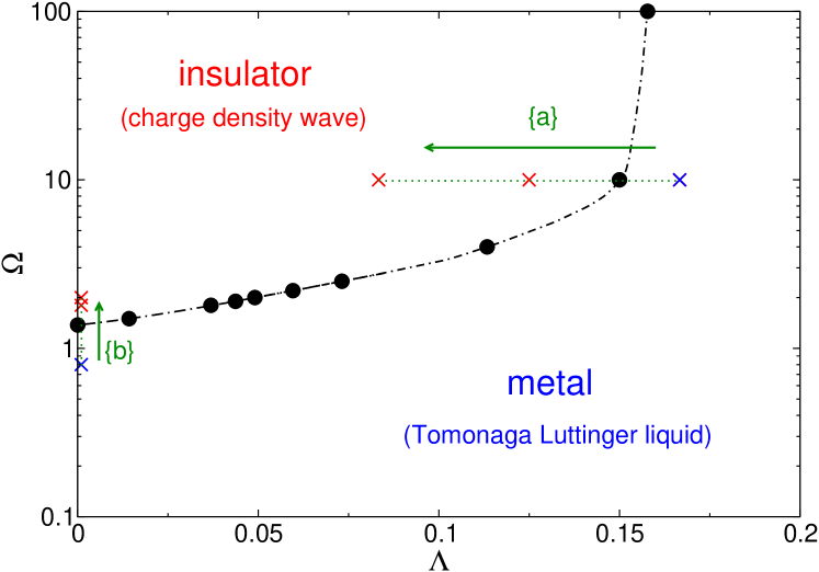
Figure 1: (Color online) DMRG phase diagram of the two-channel fermion-boson transport model (1) [see also Eq. (6)] for the 1D half-filled band case (the dot-dashed line is a guide to the eye). The crosses mark the parameter values used within our PRM calculation when passing the TLL$\to$CDW transition at fixed $\Omega=10$ {a} and $\Lambda=0.001$ {b} (green arrows), respectively.

Concerning the nature of the metal-insulator quantum phase transition, it is a moot point, whether the TLL-CDW crossover in the half-filled fermion-boson model (1), taking place at relatively large $\Omega$, bears some resemblance to the usual Peierls transition in the spinless fermion Holstein model Bursill et al. (1998); Sykora et al. (2005); Hohenadler et al. (2006); Ejima and Fehske (2009). In this regard the question of boson softening will certainly be of importance.

III.2 CDW order parameter

To analyze the nature of the metal-insulator transition of (1) in more detail, we calculate in the following a set of characteristic quantities by the PRM for the (1D half-filled) infinite system. Thereby we cross the TLL$\to$CDW transition in the following figures at fixed $\Omega$ [panels (a)] and $\Lambda$ [panels (b)] (cf. Fig. 1 lines {a} and {b}, respectively). As for the half-filled Holstein model Sykora et al. (2009), the CDW structure of the insulating state shows up in the correlation function $d_{k}^{c}=\langle c_{k}^{\dagger}c_{k+Q}\rangle$, which can be considered as CDW order parameter.

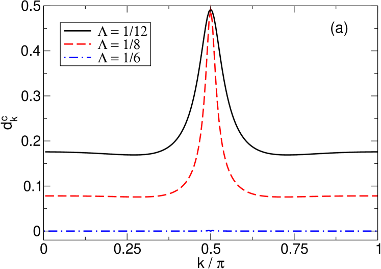
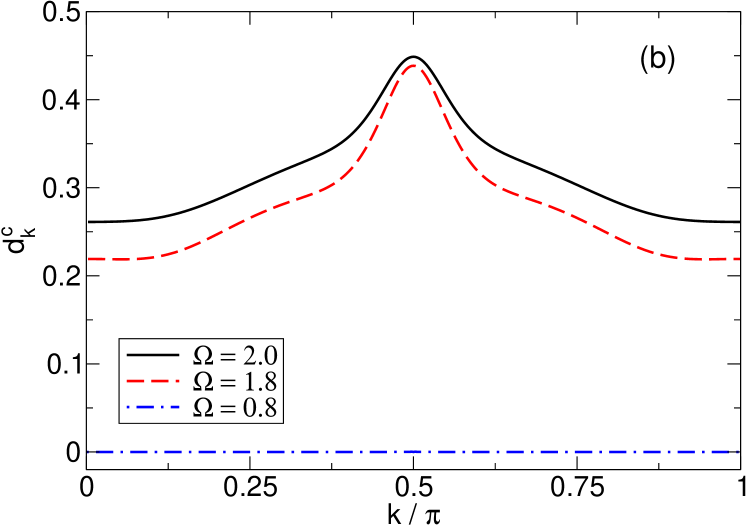
Figure 2: (Color online) Zero-temperature expectation value $d_{k}^{c}$, indicating CDW order in the half-filled fermion-boson model (1), at $\Omega=10$ [upper panel (a)] and $\Lambda=0.001$ [lower panel (b)].

Figure 2 displays the variation of this expectation value when the wave vector $k$ runs through the half 1D Brillouin zone. Obviously we have $d_{k}^{c}=0$ in the metallic phase (blue dot-dashed line). Entering the CDW state $d_{k}^{c}$ acquires finite values, whereby the maximum of $d_{k}^{c}$ is at $k=\pi/2$ (for this case $Q=\pi$ connects both Fermi momenta $k_{F}=\pm\pi/2$). If the charge order is perfect (the particles are localized in an A-B structure without any charge fluctuations, i.e. the lower and upper bands are flat), we find $d_{k}^{c}=1/2$ for all $k$. This tendency becomes apparent by comparing the results obtained in the CDW phase for different $\Lambda$ (cf. upper panel $\Lambda=1/8,\;1/12$ and lower panel $\Lambda=1/1000$; recall that $\Lambda$ describes the ability of the background to relax.)

III.3 Fermion dispersion and quasiparticle weight

Next we investigate the renormalization of the fermionic band structure,

$$E_{k}=\frac{\tilde{\varepsilon}_{k}+\tilde{\varepsilon}_{k+Q}}{2}\pm\sqrt{\Big{(}\frac{\tilde{\varepsilon}_{k}-\tilde{\varepsilon}_{k+Q}}{2}\Big{)}^{2}+|\tilde{\Delta}_{k}|^{2}}\,,$$ (53)

see Fig. 3. In the metallic regime, of course, there is no gap at the Fermi energy (Fermi vector $k_{F}=\pi/2$), and $\tilde{\Delta}_{k}$, given in the inset, is zero for all $k$.

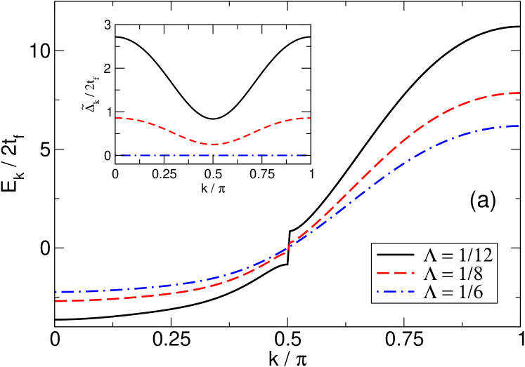
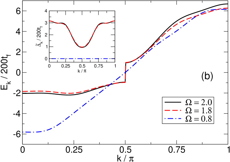
Figure 3: (Color online) Dispersion of the occupied lower (empty upper) quasiparticle band $E_{k}$ with $k\leq\pi/2$ ($k>\pi/2$) for $\Omega=10$ [panel (a)] and $\Lambda=0.001$ [panel (b)] (the Fermi energy sets the zero-point of energy). Note that band energies are differently scaled by $2t_{f}$ and $200t_{f}$ in (a) and (b). The insets show the $k$-dependence of $\tilde{\Delta}_{k}$.

While for $2\Lambda\gg\Omega$ the free transport channel ($\propto t_{f}$) dominates even when $\Omega$ is large (see Eq.(7)), the bosonic degrees of freedom will strongly affect the transport for small $\Lambda$. As a consequence, ‘coherent’ transport takes place on a strongly reduced energy scale only (we have $t_{f}/t_{b}=1/30$ [$t_{f}/t_{b}=1/400$] for the blue dot-dashed line in panel (a) [(b)]).

The coefficient $\tilde{\alpha}_{k}^{2}$, depicted in Fig. 4, gives the weight of the corresponding coherent part of the single-particle spectral function (48). $A^{-}_{k}(\omega)$ can by probed by angle-resolved photoemission experiments. At very large $\Omega$ (and small $\Lambda$), the particles will solely move by the above mentioned six-step process (52). Then the resulting ‘quasiparticle weight’, $\tilde{\alpha}_{k}^{2}$, is nearly one [see Fig. 4 (a)], and shows a very weak $k$-dependence. For small $\Omega<\Omega_{c}$ we enter the fluctuation-dominated regime and the nature of the metallic state changes noticeably. In accordance with recent dynamical DMRG data for the single-particle spectra, which show that the absorption spectrum is over-damped near $k=0,\,\pi$ because of intersecting bosonic excitations, we find $\tilde{\alpha}_{k}^{2}\sim 1$ in the vicinity of $k_{F}$ only [cf. Fig. 3 in Ref. Ejima and Fehske, 2009 and Fig. 4 (b), blue dot-dashed line].

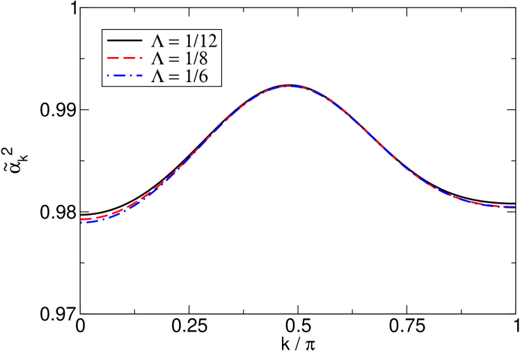
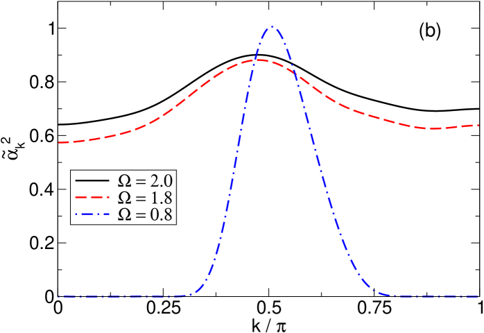
Figure 4: (Color online) Spectral weight, $\tilde{\alpha}_{k}^{2}$, of the coherent (quasiparticle) part of the electronic one-particle spectral function (48). We have $\Omega=10$ in panel (a) and $\Lambda=0.001$ in panel (b). Notations are as in Fig. 3.

In the insulating regime, the renormalized band structure $E_{k}$ is gaped (see Fig. 3, dashed and solid lines). The inset in Fig. 3 clearly shows an increase of the gap at $k=k_{F}$ as $\Lambda$ gets smaller. Note that the size of the gap is equal to $2\tilde{\Delta}_{k_{F}}$. While $\tilde{\Delta}_{k}$ is symmetric around $k=\pi$, $E_{k}$ is not. The reason is that doping a perfect CDW, states with one particle removed are connected by the six-step hopping process (52), whereas a two-step hopping process relates states with an additional particle Wellein et al. (2008). In this way the collective particle-boson dynamics leads to a more pronounced flattening of the coherent band for $k<k_{F}$, i.e., the widths of the highest photoemission and lowest inverse photoemission band differ Wellein et al. (2008); Ejima and Fehske (2009). It is encouraging that our analytic PRM approach reproduces this non-trivial correlation-induced (mass-) asymmetry. Let us emphasize that the $\tilde{\alpha}_{k}^{2}$ given in Fig. 4 for the CDW case (dashed and solid curves) belong to the highest photoemission band in the whole interval $[0,\pi]$ (the corresponding $E_{k}$ is not depicted in the region $\pi/2<k\leq\pi$ in Fig. 3). Compared to the metallic phase the spectral weight of the lower CDW band is significantly changed for intermediate-to-small boson frequencies only.

III.4 Boson dispersion and occupation numbers

The Einstein bosons, describing excitations of the background, gain a dispersion owing to the coupling to the fermions. The renormalization of the boson dispersion, $\tilde{\omega}_{q}/\omega_{b}$, is displayed in Fig. 5. It is rather weak for large $\Omega$ in both the metallic and insulating states. For smaller boson frequencies, we find a strong renormalization in the TLL phase (up to 50% for $\Omega=0.8$) at larger momenta [see dot-dashed curve in panel (b)]. This is in accordance with the over-damped single-particle excitations observed in the ARPES spectra Ejima and Fehske (2009) and, of course, also shows up in the depletion of $\tilde{\alpha}_{k}^{2}$ away from $k=\pi/2$ [see Fig. 4 (b)].

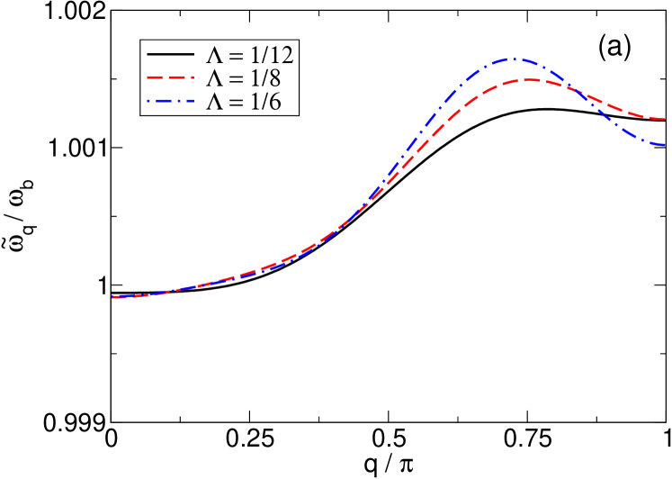
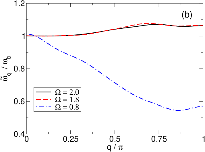
Figure 5: (Color online) Renormalized boson frequencies $\tilde{\omega}_{q}$ for the fermion-boson transport model (1) with $\Omega=10$ [panel (a)] and $\Lambda=0.001$ [panel (b)].

Most notably, for the CDW state, we observe a hardening of the boson modes near the Brillouin zone boundary. This holds in the whole $\Omega$ region and means that the TLL$\to$CDW transition is unlike the usual displacive Peierls transition which, in general, is accompanied by the softening of the $q=\pi$ boson (phonon) Sykora et al. (2005); Hohenadler et al. (2006). In our case, the CDW state is driven by the stiffness of the background, being most pronounced at large $\Omega$ and small $\Lambda$. By contrast, when $\Omega$ is small, i.e. the background readily fluctuates, the kinetic energy part will naturally overcompensate any potential energy gain by charge ordering. Another reason for the absence of boson softening might be the particular form of the fermion-boson interaction. As can be seen from the Fourier transformed Hamiltonian (8), the fermion-boson coupling vanishes for $k=\pm\pi/2$, i.e., precisely for the Fermi momenta of the half-filled band case.

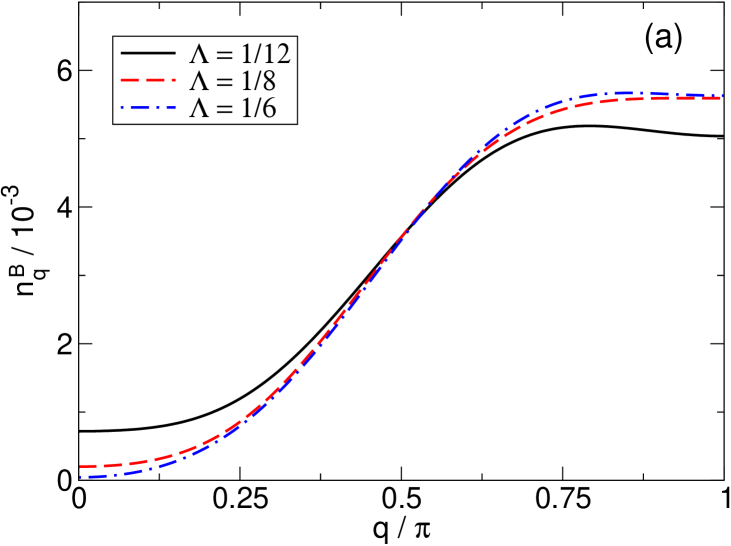
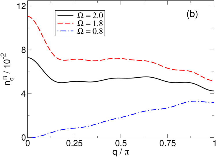
Figure 6: (Color online) Transformed boson expectation value $n_{q}^{B}=\langle B^{\dagger}_{q}B_{q}\rangle$ at $\Omega=10$ (a) and $\Lambda=0.001$ (b).

It may be worthwhile to demonstrate that our PRM approach has the advantage that all features of the results for $\tilde{\omega}_{q}$ and all other renormalized quantities can easily be understood on the basis of the former renormalization equations. For simplicity we shall restrict ourselves to the renormalization of $\tilde{\omega}_{q}$ in the case of large $\Omega$. In this regime, from Eq.(27) one may point out the stiffening of the boson modes. Since the boson energy $\omega_{b}$ is much larger than the electronic bandwidth, for all $\lambda$ a positive energy denominator $(\varepsilon_{k,\lambda}-\varepsilon_{k+q,\lambda}+\omega_{q,\lambda})$ is obtained. Nevertheless, in the $k$ sum on the right hand side of Eq.(27) there are as many negative as positive terms due to the factor $(n_{k}^{c}-n_{k+q}^{c})$. Since from $(n_{k}^{c}-n_{k+q}^{c})<0$ it follows that $(\varepsilon_{k,\lambda}-\varepsilon_{k+q,\lambda})>0$, the negative terms have larger energy denominators and are always smaller than the positive terms. The resulting renormalization of $\tilde{\omega}_{q}$ is therefore positive for all $q$ values and largest for $q=\pi$ due to the smallest energy denominator. Furthermore, since $g_{k}\propto t_{b}$ and $\omega_{b}$ is large the renormalization contributions in Eq. (27) are of the order of $t_{b}^{2}/\omega_{b}=\omega_{b}/\Omega^{2}\ll\omega_{b}$ which gives rise to the weak dispersion of $\tilde{\omega}_{q}$ observed in Fig. 5. For smaller values of $\Omega$ the bosonic and fermionic energy values in the denominator of Eq. (27) can become comparable which immediately leads to a strong dispersion of $\tilde{\omega}_{q}$ (see dot-dashed curve in Fig. 5 and solid curve in Fig. 8).

Figure 6 gives the ($q$-resolved) boson occupation numbers. As one can see from Eq. (II.2.2), this quantity for $T=0$ acquires finite values solely by coupling to fermionic degrees of freedom. Note that the first term in Eq. (II.2.2) vanishes for $T=0$. We see that the formation of the CDW state is accompanied by a finite occupation value of the $q=0$ boson mode, which is about two orders of magnitude larger if one compares $n_{0}^{B}$ for the CDWs established at $\Omega=1.8$ and $\Omega=10$, respectively. Different from the Holstein-model CDW (Peierls) phase Sykora et al. (2005), the CDW phase of the half-filled fermion-boson transport model (1) is always a few-boson state however. Referring to this, our PRM results corroborate previous small cluster exact diagonalization data Wellein et al. (2008). As can be seen from the third term of Eq. (II.2.2), bosons having finite momentum give rise to an effective fermion interaction on neighboring sites.

IV Spectral properties

While the fermionic single-particle spectral function of the transport model (1) was previously calculated for finite clusters by exact diagonalization Wellein et al. (2008) and dynamical DMRG Ejima and Fehske (2009) techniques, the spectral response of the bosons has not been studied so far. The PRM allows to investigate the interrelation between fermion and boson dynamics by computing the boson spectral function, $C_{q}(\omega)$, according to Eq. (47), for the 1D infinite system Sykora et al. (2006).

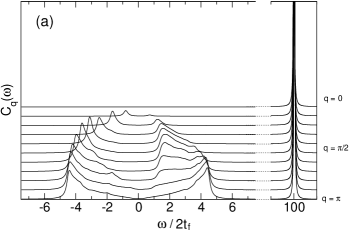
Figure 7: Boson spectral function $C_{q}(\omega)$ of the half-filled fermion-boson transport model (1) with: $\Omega=10$, $\Lambda=1/4$ [panel (a)]; $\Omega=1/150$, $\Lambda=1/90$ [panel (b)]; $\Omega=4$, $\Lambda=1$ [panel (c)]; $\Omega=4$, $\Lambda=2$ [panel (d)]. The frequency $\omega$ is given in units of $2t_{f}$.

Figure 7 shows $C_{q}(\omega)$ in the metallic regime, for different $\Omega$ and $\Lambda$ parameters. For very large $\Omega=10$ [panel (a)], the boson energy is hardly renormalized by the coupling to the fermions. Accordingly we observe a strong signal at the bare boson frequency $\Omega/2t_{f}=100$ (first term in Eq. (47); the second term in Eq. (47) will not contribute because there are no states available with $\omega=-\Omega/2t_{f}$). The third term in Eq. (47) detects particle-hole excitations and leads to the two incoherent absorption bands in $C_{q}(\omega)$ running from $q=0\to\pi$ with energies between $\omega=0$ and $\omega\simeq\pm 10t_{f}=\pm t_{b}/2$. At small $\Omega=0.00\bar{6}$, see panel (b), the (one-) boson excitation is located within the fermionic band. As a result we find a strong renormalization of the bare boson frequency (see also $\tilde{\omega}_{q}$ in Fig. 8), leading to the dispersive signal in the range $\omega/2t_{f}\simeq 0.5\times 10^{-3}\ldots 10^{-3}$. We note that for $\Lambda=0.0\bar{1}$ used in panel (b) the fermion-boson coupling is small in comparison with the free fermion bandwidth (we have $g_{k}/\varepsilon_{k}=t_{b}/t_{f}=0.3$ in the model (8)), hence the effect of multi-boson absorption processes is negligible. The lower two panels of Fig. 7 demonstrate how $\Lambda$ affects the boson absorption at fixed $\Omega$. In panel (c), for $\Lambda=1$ and $\Omega=4$, the boson frequency is larger by a factor of two than the ‘free’ fermion bandwidth ($4t_{f}=2$), whereas they have the same size for the $C_{q}(\omega)$ spectrum with $\Lambda=2$ shown in panel (d). Quite differently, in the former case, the bare boson mode hardens, while it softens near $Q=\pi$ in the latter case, where the fermion and boson degrees of freedom are strongly mixed. This becomes even more visible by comparing the corresponding (dashed and solid) $\tilde{\omega}_{q}$ curves in Fig. 8.

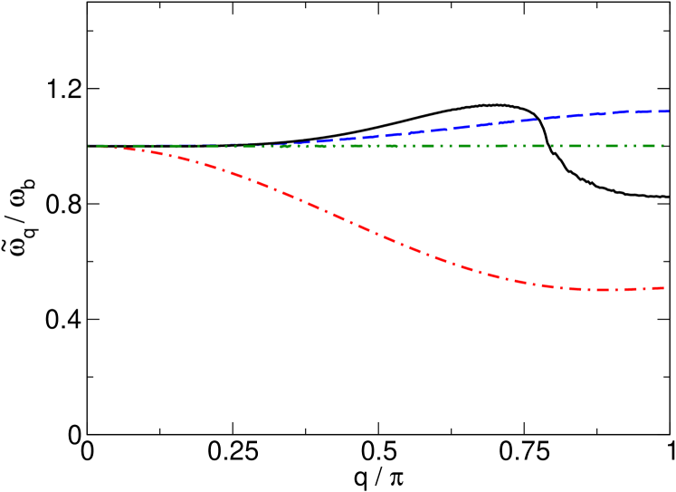
Figure 8: (Color online) Renormalized boson frequencies for the parameters used in Fig. 7: $\Omega=10$, $\Lambda=1/4$ (green double-dot-dashed line; $\Omega=1/150$, $\Lambda=1/90$ (red dot-dashed line); $\Omega=4$, $\Lambda=1$ (blue dashed line), $\Omega=4$, $\Lambda=2$ (black solid line).

V Conclusions

To summarize, we adapted the projective renormalization method to the investigation of a novel two-channel fermion-boson model, describing charge transport within a background medium. By large-scale numerical DMRG studies this model has been proven to show a metal-insulator quantum phase transition for the one-dimensional half-filled band case. The transition is triggered by strong correlations evolving in the background and typifies as a Luttinger-liquid charge-density-wave crossover.

Our analytical approach captures this TLL-CDW transition for the infinite system, without truncating the bosonic Hilbert space as in purely numerical investigation schemes. Therefore, the PRM is particularly well suited to analyze the bosonic degrees of freedom when passing the metal-insulator phase boundary.

In the course of the renormalization procedure of the fermion-boson Hamiltonian we end up with a model of noninteracting—but dressed—electrons and bosons. In this way, the renormalization of the fermion band dispersion and of the boson frequency is obtained, and various ground-state expectation values were calculated. Moreover, we derived analytical expressions for the single-particle (inverse) photoemission spectra and for the boson spectral function, which allows us to pinpoint the most important absorption and emission processes during particle transport, and throws some light on the nature of the TLL-CDW transition.

In particular, we show that the insulating CDW phase, realized for large boson frequencies $\Omega$ and small boson relaxation parameter $\Lambda$, is characterized by a gapful, mass asymmetric band structure. Thereby the lower occupied band is almost flat by reason that transport is only possible through a vacuum restoring six-step hopping process. The CDW phase is a few-boson state. By contrast, the metallic (TLL) phase is a many-boson state, especially for small $\Omega$, where the background heavily fluctuates. Note that this regime is not that easy accessible by numerical approaches. Here we observe a well-defined electron band in the vicinity of $k_{F}$ only. Due to many intersecting boson branches the (inverse) photoemission spectra are ‘overdamped’ near the Brillouin zone boundaries.

The boson spectral function and renormalized boson dispersion clearly indicate that the TLL-CDW transition is not accompanied by a softening of the zone-boundary boson mode. Rather a harding of the $Q=\pi$ boson is observed. This might be partially attributed to the vanishing Fourier-transformed fermion-boson coupling term at wave-numbers $\pm\pi/2$, which denote the two Fermi points for the half-filled band case. The situation changes if we look for a metal-insulator transition for other commensurate band-filling factors, e.g., at quarter filling. Whether the system there undergoes a soft-mode transition for small $\Omega$ is an interesting open question that deserves future efforts. In this connection other kinds of charge-ordered states should be also considered.

References

- Grüner (1994) G. Grüner, Density Waves in Solids (Addison Wesley, Reading, MA, 1994).
- Bishop and Swanson (1993) A. R. Bishop and B. I. Swanson, Los Alamos Sciences 21, 133 (1993).
- Su et al. (1979) W. P. Su, J. R. Schrieffer, and A. J. Heeger, Phys. Rev. Lett. 42, 1698 (1979).
- Holstein (1959) T. Holstein, Ann. Phys. (N.Y.) 8, 325 (1959).
- Bursill et al. (1998) R. J. Bursill, R. H. McKenzie, and C. J. Hamer, Phys. Rev. Lett. 80, 5607 (1998).
- Hohenadler et al. (2006) M. Hohenadler, G. Wellein, A. R. Bishop, A. Alvermann, and H. Fehske, Phys. Rev. B 73, 245120 (2006).
- Peierls (1955) R. Peierls, Quantum theory of solids (Oxford University Press, Oxford, 1955).
- Hubbard (1963) J. Hubbard, Proc. Roy. Soc. London, Ser. A 276, 238 (1963).
- Mutou et al. (1998) T. Mutou, N. Shibata, and K. Ueda, Phys. Rev. B 57, 13702 (1998).
- Takada and Chatterjee (2003) Y. Takada and A. Chatterjee, Phys. Rev. B 67, 081102(R) (2003); H. Fehske, M. Kinateder, G. Wellein, and A. R. Bishop, Phys. Rev. B 63, 245121 (2001); H. Fehske, G. Wellein, G. Hager, A. Weiße, and A. R. Bishop, Phys. Rev. B 69, 165115 (2004); R. T. Clay and R. P. Hardikar, Phys. Rev. Lett. 95, 096401 (2005); S. Bissola and A. Parola, Phys. Rev. B 73, 195108 (2006).
- Wohlfeld et al. (2009) K. Wohlfeld, A. M. Oleś, and P. Horsch, Phys. Rev. B 79, 224433 (2009).
- Berciu (2009) M. Berciu, Physics 2, 55 (2009).
- Komineas et al. (2007) S. Komineas, G. Kalosaka, and A. R. Bishop, Phys. Rev. E 65, 061905 (2007).
- Edwards (2006) D. M. Edwards, Physica B 378-380, 133 (2006).
- Alvermann et al. (2007) A. Alvermann, D. M. Edwards, and H. Fehske, Phys. Rev. Lett. 98, 056602 (2007).
- Wellein et al. (2008) G. Wellein, H. Fehske, A. Alvermann, and D. M. Edwards, Phys. Rev. Lett. 101, 136402 (2008).
- Ejima et al. (2009) S. Ejima, G. Hager, and H. Fehske, Phys. Rev. Lett. 102, 106404 (2009).
- Ejima and Fehske (2009) S. Ejima and H. Fehske, Phys. Rev. B 80, 155101 (2009).
- Hübsch et al. (2008) A. Hübsch, S. Sykora, and K. W. Becker (2008), preprint, URL arXiv:0809.3360; K. W. Becker, A. Hübsch, and T. Sommer, Phys. Rev. B 66, 235115 (2002).
- Wegner (1994) F. Wegner, Ann. Phys. (Leipzig) 3, 77 (1994).
- Hübsch and Becker (2005) A. Hübsch and K. W. Becker, Phys. Rev. B 71, 155116 (2005).
- Sykora et al. (2005) S. Sykora, A. Hübsch, K. W. Becker, G. Wellein, and H. Fehske, Phys. Rev. B 71, 045112 (2005).
- Becker et al. (2007b) K. W. Becker, S. Sykora, and V. Zlatic, Phys. Rev. B 75, 075101 (2007b).
- (24) S. Ejima, private communication.
- Sykora et al. (2009) S. Sykora, A. Hübsch, and K. W. Becker, Europhys. Lett. 85, 57003 (2009).
- Sykora et al. (2006) S. Sykora, A. Hübsch, and K. W. Becker, Europhys. Lett. 76, 644 (2006).