High Resolution X-Ray Spectroscopy of SN 1987 A: Monitoring with XMM-Newton

Abstract

Context. We report the results of our XMM-Newton monitoring of SN 1987 A. The ongoing propagation of the supernova blast wave through the inner circumstellar ring caused a drastic increase in X-ray luminosity during the last years, enabling detailed high resolution X-ray spectroscopy with the Reflection Grating Spectrometer.

Aims. The observations can be used to follow the detailed evolution of the arising supernova remnant.

Methods. The fluxes and broadening of the numerous emission lines seen in the dispersed spectra provide information on the evolution of the X-ray emitting plasma and its dynamics. These were analyzed in combination with the EPIC-pn spectra, which allow a precise determination of the higher temperature plasma. We modeled individual emission lines and fitted plasma emission models.

Results. Especially from the observations between 2003 and 2007 we can see a significant evolution of the plasma parameters and a deceleration of the radial velocity of the lower temperature plasma regions. We found an indication (3$\sigma$-level) of an iron K feature in the co-added EPIC-pn spectra.

Conclusions. The comparison with Chandra grating observations in 2004 yields a clear temporal coherence of the spectral evolution and the sudden deceleration of the expansion velocity seen in X-ray images $\sim$6100 days after the explosion.

1 Introduction

The circumstellar ring system around SN 1987 A was ejected by the progenitor star approximately 20 000 years before the supernova explosion. About 10 years after the explosion the blast wave started to propagate through the inner ring, causing compression, heating and ionization of its matter. At that time bright unresolved regions, so called hot spots, appeared all around the ring in HST images (Lawrence et al. 2000) and the rather linear increase in the soft X-ray band, as observed with ROSAT since 1992 (Beuermann et al. 1994; Hasinger et al. 1996), was followed by an exponential brightening as monitored with XMM-Newton, Chandra, Suzaku and Swift. Recently, some flattening of the flux increase is seen (Sturm et al. 2009, and references therein for the individual fluxes).

The X-ray spectra are interpreted as thermal emission composed of a lower temperature component ($\sim$0.5 keV) and a higher temperature component ($\sim$2.5 keV). Deep Chandra grating observations allowed the measuring of the bulk gas velocity due to spectral line deformation. Surprisingly these values were lower than the velocities expected from the plasma temperatures. This suggests the contribution of reflected shocks, additional to the ’normal’ forward shock (Zhekov et al. 2005, 2006, 2009; Dewey et al. 2008). The expansion velocity derived from Chandra X-ray images is even higher. About 6100 days after the explosion a sharp deceleration to 1600$-$2000 km s^-1 was observed (Racusin et al. 2009).

Shocks transmitted into denser regions of the ring have a slower shock wave velocity and therefore can be responsible for the low temperature component. This interpretation is supported by the morphology seen in optical and X-ray images (McCray 2007), as well as the similar evolution of the soft X-ray flux (0.5-2.0 keV) and the evolution of highly ionized optical emission lines from the hot spots (Gröningsson et al. 2006). This emission might be caused by even slower radiative shocks.

Renewed radio emission of SN 1987 A was detected in July 1990 (Turtle et al. 1990). A continuously rising flux and increasing source radius has been observed by the ATCA since then (Gaensler et al. 2007; Ng et al. 2008). The increase of the radio light curve matches the evolution of the hard X-ray flux (2-10 keV) quite closely (Park et al. 2005; Aschenbach 2007), thus the synchrotron radio emission may originate in the hot thermal plasma between the forward and reverse shock and a fraction of the hard X-ray flux may also have a non-thermal origin. Broad H${\alpha}$ and Ly$\alpha$ lines suggest the presence of the reverse shocks (Michael et al. 2003; Heng et al. 2006).

This study reports on the yearly XMM-Newton monitoring observations of SN 1987 A between January 2007 and January 2009 together with one prior observation from May 2003, making it possible to reveal the detailed plasma evolution. We measured light curves and widths of individual emission lines and analyzed the spectral plasma evolution by fitting thermal plasma emission models.

2 Observations and Data Reduction

Table 1: XMM-Newton observations of SN 1987 A and data selection.

Date	Time	Satellite	Instrument	Read-out	Filter	Net Exp	Counts(a)
	(UT)	Revolution		Mode		[s]
2003 May 10-11	16:41-23:37	0626	EPIC-pn	SW, 6ms	medium	34983	13712
	11:42-23:38		RGS1	Spectro	-	112164	3061
	10:47-23:38		RGS2	Spectro	-	111671	3635
2007 Jan 17-19	19:28-01:18	1302	EPIC-pn	FF, 73ms	medium	72478	117055
	18:23-01:19		RGS1	Spectro	-	110528	7797
	18:23-01:18		RGS2	Spectro	-	110475	11989
2008 Jan 11-13	21:32-04:07	1482	EPIC-pn	FF, 73ms	medium	79549	166180
	20:30-04:14		RGS1	Spectro	-	113617	10022
	20:30-04:14		RGS2	Spectro	-	113846	15921
2009 Jan 30-31	18:40-22:27	1675	EPIC-pn	FF, 73ms	medium	72925	185071
	18:17-22:36		RGS1	Spectro	-	101312	11528
	18:17-22:36		RGS2	Spectro	-	101547	17346

^(a)Net. counts in the $0.53-10.0$ keV (EPIC-pn) and 0.35$-$2.1 keV (RGS) band

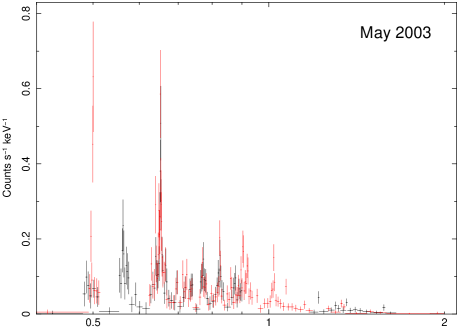
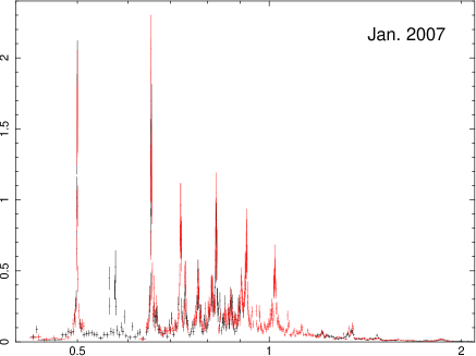
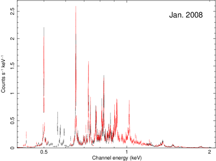
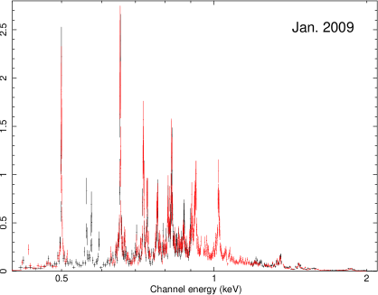
Figure 1: The RGS1 (black) and RGS2 (red) spectra of SN 1987 A observations in 2003, 2007, 2008 and 2009. A clear evolution in emission line ratios is seen. E.g. compare the nearly absent Fe xvii lines at $\sim$$0.72\leavevmode\nobreak\ keV$ in 2003 to the strong lines seen in the later observations. Also the Ne x Ly_α (1.02 keV) flux increases relative to the Ne ix triplet ($\sim$0.91 keV).

Since January 2007 we have performed a yearly monitoring of SN 1987 A using XMM-Newton (Jansen et al. 2001). Including an earlier observation from May 2003, four observations with an exposure each exceeding 100 ks were accomplished. A summary is listed in Table 1. Earlier observations and the May 2003 data were already analyzed by Haberl et al. (2006), and Heng et al. (2008) evaluated the Jan. 2007 observation concentrating on the elemental abundances. In this study we use consistent models to analyze the two new observations in combination with the previous data, to obtain the evolution of the X-ray spectra as seen by the Reflection Grating Spectrometer (RGS, den Herder et al. 2001). To extend the X-ray band up to 10 keV, we included also the EPIC-pn (Strüder et al. 2001) spectra in our analysis.

We used XMM-Newton SAS 8.0.0 to process the data. For the extraction of EPIC-pn spectra, single-pixel events in good time intervals (GTIs) with low background (threshold at 8 cts s^-1 arcmin^-2) were selected from the source region, centered on SN 1987 A, and a point source free background region, each with a radius of 30″. The RGS spectra were obtained using rgsproc, and GTIs (RATE $<$ 2.0) were used to select low background intervals. In the 2003 observation, the Honeycomb nebula is located on the dispersion axis. Using the intrinsic energy resolution of the RGS Focal Plane Camera CCDs, counts from the Honbycomb nebula are excluded. For the other three observations, the Honeycomb nebula lies at the cross-dispersion axis at the very rim of the CCDs. By comparing our background spectra with the RGS background model (created by rgsbkgmodel), we find no significant contribution from the Honeycomb nebula to the background spectra.

To obtain a detailed spectrum with $\sim$438 ks exposure, the RGS spectra of the four observations were added with rgscombine, which also calculates combined response files. To allow proper application of the $\chi$-statistics, all spectra are binned to have at least 30 (RGS) or 20 (EPIC-pn) counts per bin. Due to the high statistics of the RGS-spectra a binning of 30 cts/bin does not influence most emission lines which have far more than 30 cts in most bins. thus there is no influence on the measured line parameters.

3 Spectral Analysis

Spectral fitting was performed using XSPEC (Arnaud 1996) version 12.5.0x. The errors are given for certain $\Delta\chi^{2}$ ranges. Generally, $\Delta\chi^{2}=2.71$ is associated with the 90% confidence range for one parameter of interest.

3.1 Identification of Emission Lines

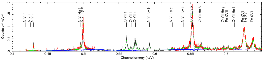
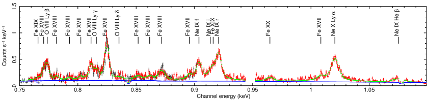
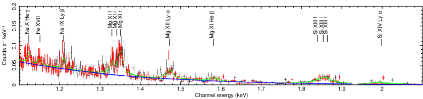
Figure 2: Co-added RGS1 (black) and RGS2 (red) spectra from all 4 observations of SN 1987 A together with the best fit empirical model (green) and the absorbed bremsstrahlung continuum (blue). The line labels mark the strongest lines as expected from the two component vpshock model at the best fit energy of the line center.

Since the RGS spectra of SN 1987 A are dominated by emission lines (see Fig. 1), we first identified the individual lines using the co-added spectra. We constructed an empirical model and fitted it to the combined RGS1 and RGS2 spectra simultaneously.

As quasi-continuum we used a thermal bremsstrahlung model with absorption, which is formally a good approximation to the observed continuum, containing also radiative recombination and two photon decays. This component also represents various weak emission lines, which are not resolved in the RGS spectra. A constant factor was allowed to vary between the two RGS spectra. We first fitted the strong lines with Gaussian profiles. The high statistical quality of the summed spectrum required the introduction of further weak lines where we noticed residua. Our final model comprises 53 lines as listed in Table 2. Fitted to the co-added spectra, all lines have a normalization inconsistent with 0 for $\Delta\chi^{2}=2.71$ (except for the intercombination lines of helium-like N and Mg). For line complexes the line energies were combined to one value according to their ratio in ATOMDB 1.3.1 and the line widths were linked. For weak lines it was not possible to fit individual line widths, thus we coupled them with the next strong line. We get a best fit with $\chi^{2}/{\rm dof}=1843/1465$. The summed RGS spectra are shown in Fig. 2 together with the best fit model and the bremsstrahlung quasi-continuum (kT$=402_{-6}^{+5}$ eV). The line labels mark the best fit energy of the fitted Gaussian and name the strongest emission line expected from plane-parallel shocked plasma emission codes (see below) at this energy. With these identifications we obtain line shifts consistent with a systemic redshift of $349\pm 24$ km s^-1(see Fig. 3).

Figure 3: Line shifts according to the empirical model. The horizontal line shows the best fit for a systemic redshift. Errors are for $\Delta\chi^{2}=2.71$ confidence range.

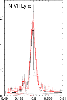
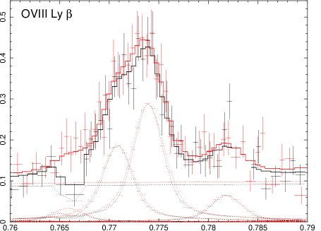
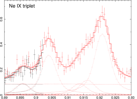
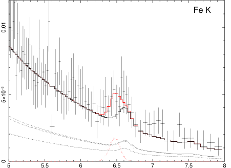
Figure 4: Examples for emission line complexes from the summed spectra: N vii Ly _α, O viii Ly_β and the Ne ix triplet as seen by the RGS1 (black) and RGS2 (red). Also the empiric model and its components are plotted. In the right panel an indication for a Fe K feature is seen in the summed EPIC-pn spectrum of the newer three observations. A sum of the high temperature component plane-parallel shock models derived from the individual observations (black) is compared with a model containing an additional Gaussian (red). Horizontal axes: Channel energy in keV, Vertical axes: Counts s^-1 keV^-1.

The high statistical quality of the co-added RGS spectra allowed us to investigate emission lines in unprecedented detail. E.g. the N vi helium-like triplet at $\sim$0.42 keV is clearly seen in the summed spectra (cf. Fig. 2). Other examples of emission line complexes are shown in Fig. 4: Next to the N vii Ly_α (at 0.50 keV) line we found an additional line at slightly lower energy (see Fig. 4), most likely N vi He_β, which is the strongest line at this position in the plasma codes. But also argon lines contribute here which may cause the higher line shift. In previous analyses with lower statistics this line likely was blended with the $\sim$10 times more luminous N viii Ly_α line. The line shape at the energy of the O viii Ly_β (0.77 keV) line is inconsistent with a Gaussian profile and the line width for a single Gaussian is outstandingly higher than found for the surrounding lines (2 eV vs. 0.25 eV). Plasma models suggest two iron lines at slightly lower energies, that were included in our model. The shape of the Ne ix triplet ($\sim$0.91 keV) is also not reproducible by three Gaussians. Here Fe xix (917.1 eV) may contribute to the flux, although this line is not expected to be strong from emission codes.

For strong lines in the summed spectra, we find measured line widths inconsistent with zero within a confidence range of $\Delta\chi^{2}=2.71$, demonstrating that line broadening can be detected significantly with RGS. Also a trend of increasing width with rising energy is seen. A fit of an energy dependent line width $\sigma(E)=\sigma_{0}(E/1{\rm keV})^{\alpha}$ yields $\sigma_{0}=(1.35\pm 0.36)$ eV and $\alpha=2.05_{-0.72}^{+0.66}$. The power law index agrees well with the Chandra LEGT 2007 results (Zhekov et al. 2009).

In a second step we fitted the empirical model to the spectra of the individual observations to follow the evolution of the individual emission lines in a consistent way. Only parameters with expected time dependence, i.e. the line fluxes and the parameters of the bremsstrahlung continuum, were allowed to vary. The absorption as well as the center energy and width of the Gaussians were fixed at the values obtained from the summed spectra. Here these values can be determined more precisely than in the individual spectra. Using the RGS spectra with the best statistics (i.e. the 2009 data), we compared line widths fixed in the individual fits with those allowing line widths free in the fits. We found that 20 of 21 line widths are consistent. A time dependent analysis of the line widths is done in section 3.2, by using plasma models and assuming a power law dependence. The line fluxes with fixed and variable widths also are consistent and we conclude that the fixed line widths do not influence the derived line fluxes.

The individual line fluxes are listed in Table 2, light curves for prominent oxygen and neon lines are shown in Fig. 5. We note, that the temperature of the quasi-bremsstrahlung continuum shows a trend of an increase (254${}_{-40}^{+64}$, 413${}_{-21}^{+30}$, 436${}_{-19}^{+26}$ and 405${}_{-14}^{+17}$ for the 2003, 2007, 2008 and 2009 observation, respectively), but stress, that this component not represents bremsstrahlung only.

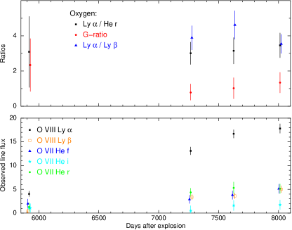
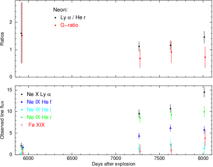
Figure 5: The lower panels show the light curves of various emission lines with fluxes in $10^{-5}$ photons cm^-2 s^-1. The upper panels show the corresponding line ratios (not absorption corrected). The G-ratio is defined as the helium like line flux ratio of $(f+i)/r$. Overlapping data points are shifted by 10 days for clarity.

We also searched for a Fe K line complex between 6.4 and 6.7 keV in a summed EPIC-pn spectrum of the three observations between 2007 and 2009, where we have a better statistics in this energy band. To characterise the feature, we fitted a bremsstrahlung continuum (kT=$(3.3\pm 0.5)$ keV, $EM=(1.3\pm 0.3)\times 10^{58}$cm^-3) and one Gaussian in the 4.0$-$10.0 keV band.

The best fit Gaussian centre energy is (6.57$\pm$0.08) keV with a sigma-width of 62.7${}_{-62.7}^{+141}$ eV and the line flux is 7.3${}_{-4.2}^{+5.7}\times 10^{-7}$ photons cm^-2 s^-1. Already, Heng et al. (2008) noted a possible detection in the 2007 data, but the individual EPIC-pn and the summed EPIC-MOS spectra have not enough statistics for a detailed analysis. With increasing ionization, the centroid energy of the Fe K line complex is shifted from the 6.4 keV fluorescent line over various ionization stages to the He-like emission of Fe xxv at $\sim$6.7. To account for this effect, we fitted an exposure weighted sum of the plane-parallel shock model derived for the high temperature component in Sect. 3.2, but used NEI-model version 1.1, which contains also Fe-ions less ionized than He-like. We only allowed a constant factor to account for the normalization and obtained a flux of the iron K lines from the shocked plasma of $4.9\times 10^{-7}$ photons cm^-2 s^-1. As can be seen in the right panel of Fig. 4, the resulting line shape does not explain the observed feature at the lower energy side. We investigated the possibility of an additional line with zero width (also shown in Fig. 4). The best fit values are $4.7\pm 3.3\times 10^{-7}$ photons cm^-2 s^-1 at a centre energy of 6.48${}_{-0.12}^{+0.17}$ keV.

Table 2: Identified lines in the RGS spectra.

Line	$E_{\rm rest}^{(a)}$ (keV)	$E_{\rm obs}^{(b)}$ (keV)	$\sigma^{(c)}$ (eV)	detected flux(d) ($10^{-6}$ photons cm-2s-1)
				2003	2007	2008	2009
N VI f	0.4198	0.4193	0.01	$<$33.8	$<$36.7	$<$31.4	20.3 $\pm$8.7
N VI i	0.4263	0.4257	0.01	$<$34.7	$<$9.5	$<$8.7	$<$13.1
N VI r	0.4307	0.4301(2)	0.01 (0$-$0.37)	$<$31.4	24.9 $\pm$10.7	29.1 $\pm$9.9	22.8 $\pm$9.0
N VI He $\beta$	0.4980	0.4965(3)	0.02 (0$-$0.74)	7.6 $\pm$6.9	9.4 $\pm$4.3	15.4 $\pm$5.0	10.6 $\pm$5.2
N VII Ly $\alpha$	0.5003	0.4997(1)	0.37 (0.26$-$0.46)	26.2 $\pm$7.9	110.9 $\pm$8.5	122.4 $\pm$9.0	134.3 $\pm$10.1
O VII f	0.5611	0.5604	0.40	19.9 $\pm$9.6	28.9 $\pm$8.6	37.9 $\pm$8.9	51.3 $\pm$9.8
O VII i	0.5686	0.5680	0.40	10.8 $\pm$9.0	$<$15.5	16.1 $\pm$10.6	17.5 $\pm$10.1
O VII r	0.5739	0.5733(1)	0.40 (0.04$-$0.65)	13.1 $\pm$8.4	43.5 $\pm$8.8	53.1 $\pm$12.2	51.3 $\pm$10.0
N VII Ly $\beta$	0.5929	0.5926(3)	0 (0$-$0.77)	$<$13.3	13.4 $\pm$6.2	22.6 $\pm$6.4	23.3 $\pm$7.6
N VII Ly $\gamma$	0.6254	0.6247(7)	0.63	$<$9.0	$<$3.7	$<$5.3	5.2 $\pm$4.7
N VII Ly $\delta$	0.6404	0.6406(8)	0.63	15.3 $\pm$5.2	$<$1.7	$<$2.3	7.2 $\pm$4.6
O VIII Ly $\alpha$	0.6537	0.6529(1)	0.63	40.5 $\pm$5.8	130.8 $\pm$8.0	167.5 $\pm$8.4	177.8 $\pm$9.9
O VII He $\beta$	0.6656	0.6650(5)	0.63 (0.46$-$0.72)	9.4 $\pm$4.9	14.2 $\pm$4.9	8.2 $\pm$4.9	16.3 $\pm$5.5
O VII He $\gamma$	0.6978	0.697(2)	0.11	5.1 $\pm$4.5	$<$4.1	6.9 $\pm$4.3	$<$2.8
Fe XVIII	0.7035	0.703(1)	0.11	$<$2.2	$<$8.2	$<$7.4	9.8 $\pm$4.4
O VII He $\delta$	0.7127	0.712(1)	0.11	$<$8.8	$\pm$6.1	5.3 $\pm$4.0	$<$3.6
Fe XVII	0.7252	0.7250	0.11	$<$13.7	54.1 $\pm$10.7	90.9 $\pm$12.5	84.9 $\pm$13.7
Fe XVII	0.7271	0.7269(1)	0.11 (0$-$0.54)	$<$6.0	29.9 $\pm$9.4	28.2 $\pm$10.1	46.1 $\pm$11.7
Fe XVII	0.7389	0.7380(2)	0.25 (0$-$0.72)	5.0 $\pm$4.4	34.4 $\pm$5.0	38.9 $\pm$5.2	49.2 $\pm$6.0
Fe XIX	0.7696	0.7658	0.20	$<$9.1	5.1 $\pm$4.4	$<$9.4	$<$10.1
Fe XVIII	0.7715	0.7708	0.20	6.7 $\pm$5.5	12.3 $\pm$5.2	24.9 $\pm$5.9	21.5 $\pm$6.6
O VIII Ly $\beta$	0.7746	0.7738(2)	0.20 (0$-$0.86)	$<$9.3	33.6 $\pm$5.6	36.2 $\pm$6.1	50.3 $\pm$7.1
Fe XVIII	0.7835	0.7817(8)	0.25	$<$9.4	6.7 $\pm$4.1	5.6 $\pm$4.3	7.7 $\pm$5.1
Fe XVIII	0.7935	0.7929(9)	0.25	$<$2.4	$<$7.1	8.6 $\pm$4.0	5.0 $\pm$4.5
Fe XVII	0.8023	0.803(1)	0.25	$<$3.6	12.6 $\pm$4.4	5.7 $\pm$4.7	$<$9.9
Fe XVII	0.8124	0.8113	0.25	$<$5.2	26.6 $\pm$5.9	44.9 $\pm$6.4	45.3 $\pm$7.2
O VIII Ly $\gamma$	0.8169	0.8159(3)	0.25 (0$-$0.78)	5.1 $\pm$4.6	15.5 $\pm$6.1	19.8 $\pm$6.6	27.3 $\pm$7.4
Fe XVII	0.8258	0.8248(1)	0.64 (0.23$-$0.89)	14.9 $\pm$4.5	82.7 $\pm$6.4	100.3 $\pm$6.9	123.5 $\pm$8.0
O VIII Ly $\delta$	0.8365	0.835(2)	1.89	$<$4.9	$<$4.5	5.2 $\pm$5.0	12.5 $\pm$5.6
Fe XVIII	0.8530	0.8517(8)	1.89	$<$3.2	11.4 $\pm$4.6	16.5 $\pm$5.0	19.4 $\pm$5.7
Fe XVIII	0.8626	0.862(1)	1.89	$<$10.0	11.3 $\pm$5.5	18.3 $\pm$5.5	13.4 $\pm$6.0
Fe XVIII	0.8726	0.8719(4)	1.89 (1.45$-$2.35)	$<$9.0	30.7 $\pm$5.1	39.9 $\pm$5.5	54.6 $\pm$6.5
Fe XVII	0.8968	0.8957	0.85	5.0 $\pm$4.7	13.4 $\pm$4.5	17.1 $\pm$4.9	14.5 $\pm$5.5
Ne IX f	0.9050	0.9039	0.85	17.0 $\pm$6.6	43.5 $\pm$7.0	61.8 $\pm$7.9	57.7 $\pm$8.8
Ne IX i	0.9148	0.9136	0.85	$<$11.8	14.6 $\pm$12.1	23.2 $\pm$13.7	$<$30.1
Fe XIX	0.9171	0.9161	0.85	$<$13.2	$<$23.7	$<$26.3	38.2 $\pm$19.0
Ne IX r	0.9220	0.9208(2)	0.85 (0.25$-$1.23)	12.9 $\pm$7.8	85.3 $\pm$11.0	92.7 $\pm$11.3	99.7 $\pm$12.8
Fe XX	0.9651	0.965(1)	1.76	$<$4.3	14.6 $\pm$5.8	20.1 $\pm$6.2	24.1 $\pm$6.9
Fe XVII	1.0108	1.009(1)	1.76	$<$9.8	17.8 $\pm$6.7	28.1 $\pm$7.6	17.7 $\pm$8.0
Ne X Ly $\alpha$	1.0219	1.0205(3)	1.76 (1.38$-$2.28)	20.8 $\pm$7.1	95.3 $\pm$9.2	107.0 $\pm$9.9	145.3 $\pm$11.5
Ne IX He $\beta$	1.0740	1.075(2)	3.76 (2.41$-$5.53)	9.4 $\pm$8.0	16.5 $\pm$7.3	24.9 $\pm$7.3	24.5 $\pm$8.0
Ne IX He $\gamma$	1.1270	1.124(3)	1.34	$<$7.4	11.2 $\pm$5.1	10.5 $\pm$5.7	7.0 $\pm$5.9
Fe XVII	1.1512	1.15(5)	1.34	$<$5.1	9.8 $\pm$3.8	10.4 $\pm$4.3	13.3 $\pm$4.7
Ne X Ly $\beta$	1.2109	1.210(2)	1.34 (0$-$3.94)	$<$10.9	$<$9.4	$<$8.3	$<$8.8
Mg XI f	1.3311	1.3297	2.25	9.0 $\pm$8.3	10.7 $\pm$5.9	13.9 $\pm$5.7	18.6 $\pm$5.9
Mg XI i	1.3431	1.3417	2.25	$<$11.8	$<$13.0	$<$8.8	$<$7.0
Mg XI r	1.3522	1.3508(9)	2.25 (0$-$3.73)	$<$15.3	25.9 $\pm$7.0	35.2 $\pm$6.7	44.4 $\pm$6.6
Mg XII Ly $\alpha$	1.4726	1.473(2)	4.25 (0$-$7.27)	$<$15.0	12.7 $\pm$4.5	21.1 $\pm$5.4	26.6 $\pm$5.7
Mg XI He $\beta$	1.5793	1.582(6)	5.01 (0$-$17.1 )	12.6 $\pm$10.0	5.6 $\pm$4.5	7.4 $\pm$5.3	6.2 $\pm$5.1
Si XIII f	1.8394	1.840	5.38	$<$31.0	$<$20.9	$<$27.4	$<$27.9
Si XIII i	1.8537	1.855	5.38	$<$33.9	$<$29.3	$<$4.96	$<$38.7
Si XIII r	1.8649	1.865(4)	5.38 (0$-$15.8 )	$<$36.3	34.4 $\pm$11.1	$<$4.68	39.8 $\pm$12.6
Si XIV Ly $\alpha$	2.0060	1.997(1)	0 (0$-$230)	$<$85.6	22.5 $\pm$12.4	19.7 $\pm$19.4	18.1 $\pm$15.8

Note: All errors are for $\Delta\chi^{2}=2.71$ confidence range. Parameters without errors were coupled to the corresponding parameter of the following line with higher energy (see text).
^(a) Rest energy of identified line according to ATOMDB 1.3.1. If the line is a multiplet, we give the energy of the strongest component.
^(b) Central energy of the fitted Gaussian.
^(c) Best fit value of Gaussian sigma width.
^(d) Detected flux for the individual observations. For fluxes consistent with 0 at $\Delta\chi^{2}\leq 2.71$ only the upper limit is given.

3.2 Plasma Evolution

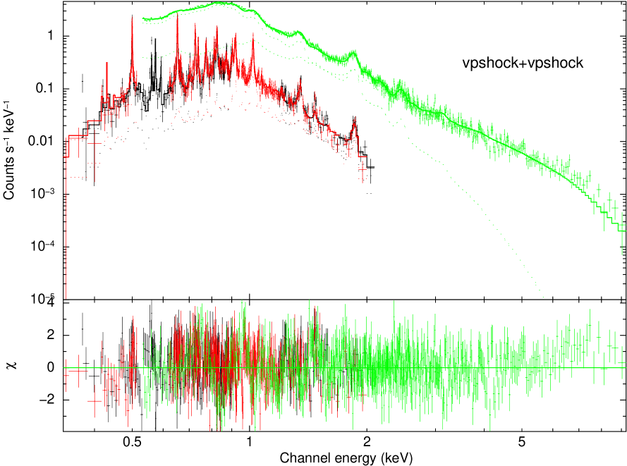
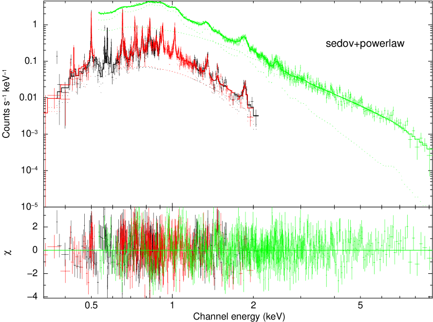
Figure 6: The XMM-Newton RGS1 (black), RGS2 (red) and EPIC-pn (green) spectra of the 2009 observation. Plotted is also a model containing two plane-parallel shock components (left panel) and a sedov+powerlaw model (right panel).

To probe the physical parameters of the X-ray emitting plasma, we fitted plasma emission models. Neither in XMM-Newton (e.g. Heng et al. 2008), nor in Chandra (e.g. Zhekov et al. 2006) observations, the spectrum was described well by just one emission component. Zhekov et al. derived a bimodal temperature distribution in differential emission measure, peaking at $\sim$0.5 keV and $\sim$2.5 keV. A non-thermal component might also contribute to the hard component (Park et al. 2005). We noticed, that the emission lines in the XMM-Newton spectra can also be described by the sedov-model in XSPEC, which has a temperature distribution according to the Sedov self-similar solution for SNRs. Here a power law is necessary for the high energy tail (cf. Fig. 6 ).

The abundances of the sedov component are significantly higher than normally found in X-ray analyses, thus we doubt the physical correctness of this component, but the model demonstrates the possible contribution of a non-thermal component up to $(1.44\pm 0.03)\times 10^{-3}$ photons keV^-1cm^-2s^-1 at 1 keV with power law index $\Gamma=3.00\pm 0.02$ (for the 2009 observation). Formally the sedov+powerlaw model results in a better fit (e.g. for the 2009 observation: $\chi^{2}_{\rm red}=1.35$ vs. $1.48$).

However, we decided to use the approximation of a plane-parallel shock structure at two temperatures as commonly found in the literature, since the sedov model is numerically slow and the RGS does not provide high resolved lines above 2.0 keV.

For a precise determination of the high temperature plasma component, we extended the energy band up to 10 keV by fitting the RGS1,2 and EPIC-pn spectra simultaneously, as it is successfully done for calibration (Plucinsky et al. 2008).

A comparison of the empiric model fitted to the 2009 RGS data and to a dataset containing also the EPIC-pn spectrum in the 0.2$-$2.0 keV energy range shows, that again 20 of 21 line widths were consistent. Because of the lower energy resolution of EPIC-pn the line widths are determined by the RGS spectra. We found inconsistent fluxes of the helium-like N vi and N vii Ly_α line between the EPIC-pn and RGS spectra. This is most likely due to calibration problems in the modeled redistribution of the EPIC-pn response at low energies. Thus we decided to limit the EPIC-pn band to 0.53$-$10 keV for this study. In future studies the $0.2-0.53$ keV EPIC-pn band with advanced calibration will yield additional information.

To derive the plasma evolution we fitted a two component plane-parallel shock model (vpshock, Borkowski et al. 2001) with NEI-version 2.0 and ionization timescale range $0<\tau<\tau_{\rm u}$. Analogous to Zhekov et al. (2009, and references therein) the chemical composition of the plasma component is assumed to be constant in time and the abundances were fitted with the exception of He (set to 2.57), C (0.09), Ar (0.54), Ca (0.34) and Ni (0.62), which produce no significant features in our data. The photo-electric absorption by the Galactic interstellar medium was set to N_H = 6$\times 10^{20}$cm^-2, whereas the LMC column density with abundances set to 0.5 for metals was a free parameter. The abundances for absorption and emission components are given according to Wilms et al. (2000), which resulted in a slightly better fit ($\chi^{2}_{\rm red}=1.32$ vs. $1.38$) than the abundances of Anders & Grevesse (1989). The main impact is on the absorption, which influences continuum emission and line ratios. We found no impact on the main results of our study. A constant factor is allowed to vary for calibration differences of the individual instruments. We modified the shock model line widths to be described by the power law function mentioned above, thus our custom version of the vpshock model contains two more parameters ($\sigma_{0}$, $\alpha$).

We fitted the four XMM observations (12 spectra) simultaneously, which results in a $\chi^{2}/{\rm dof}=5400/4084$. As best fit parameters we obtained for the LMC absorption N_H= $(2.23\pm 0.02)\times 10^{21}$ cm^-2, for the systemic velocity v${}_{\rm 87A}=326_{-16}^{+13}$ km s^-1and for the instrument dependent constants c${}_{\rm RGS2}=1.03\pm 0.01$ and c${}_{\rm pn}=1.04\pm 0.01$ (relative to c${}_{\rm RGS1}=1$). For the time dependent parameters see Table 3 and Fig. 7, for the abundances see Table 4.

Table 3: Results from the VPSHOCK+VPSHOCK model fits.

Parameter	May 2003	Jan. 2007	Jan. 2008	Jan. 2009
$kT_{1}$(keV)	0.41${}_{-0.01}^{+0.01}$	0.52${}_{-0.003}^{+0.002}$	0.53${}_{-0.001}^{+0.002}$	0.54${}_{-0.001}^{+0.002}$
$kT_{2}$(keV)	2.89${}_{-0.19}^{+0.19}$	2.43${}_{-0.06}^{+0.06}$	2.50${}_{-0.05}^{+0.05}$	2.38${}_{-0.05}^{+0.04}$
$EM_{1}^{(a)}$	4.09${}_{-0.1}^{+0.1}$	17.83${}_{-0.12}^{+0.11}$	23.45${}_{-0.12}^{+0.13}$	28.37${}_{-0.14}^{+0.15}$
$EM_{2}^{(a)}$	1.06${}_{-0.03}^{+0.03}$	2.95${}_{-0.05}^{+0.04}$	3.91${}_{-0.05}^{+0.06}$	4.91${}_{-0.07}^{+0.05}$
$\tau_{{\rm u,}1}^{(b)}$	3.25${}_{-0.26}^{+0.29}$	4.82${}_{-0.12}^{+0.14}$	6.03${}_{-0.14}^{+0.19}$	6.86${}_{-0.18}^{+0.21}$
$\tau_{{\rm u,}2}^{(b)}$	1.33${}_{-0.1}^{+0.12}$	1.93${}_{-0.1}^{+0.11}$	2.02${}_{-0.1}^{+0.09}$	2.22${}_{-0.09}^{+0.13}$
$\sigma_{0}$(eV)	3.51${}_{-0.94}^{+1.11}$	1.51${}_{-0.4}^{+0.25}$	1.58${}_{-0.29}^{+0.31}$	1.43${}_{-0.29}^{+0.33}$
$\alpha$	1.10${}_{-0.76}^{+0.74}$	2.64${}_{-0.45}^{+0.69}$	3.15${}_{-0.63}^{+0.43}$	3.10${}_{-0.52}^{+0.6}$

Note: Errors for $\Delta\chi^{2}=2.71$ confidence range.
^a EM$=\int n_{e}n_{H}dV$ in $10^{58}$ cm^-3, a distance of 50 kpc is assumed.
^b $\tau_{\rm u}$: upper limit on the ionization time range in $10^{11}$ cm^-3 s.

Table 4: Abundances of SN 1987 A

	2vpshock	sedov+po	H08	Z09	LF96	H98
N	1.385${}_{-0.057}^{+0.044}$	3.34${}_{-0.19}^{+0.34}$	0.54	0.83	2.37
O	0.128${}_{-0.002}^{+0.002}$	0.40${}_{-0.01}^{+0.01}$	0.05	0.14	0.33	0.33
Ne	0.338${}_{-0.006}^{+0.004}$	1.00${}_{-0.03}^{+0.03}$	0.20	0.41	0.63	0.41
Mg	0.291${}_{-0.007}^{+0.008}$	0.71${}_{-0.03}^{+0.04}$	0.17	0.42		0.48
Si	0.516${}_{-0.016}^{+0.018}$	1.01${}_{-0.04}^{+0.08}$	0.48	0.63	0.91	0.59
S	0.451${}_{-0.041}^{+0.039}$	1.56${}_{-0.19}^{+0.29}$	0.59	0.40	0.46	0.48
Fe	0.224${}_{-0.002}^{+0.003}$	0.46${}_{-0.01}^{+0.10}$	0.09	0.33	1.12	0.38

Note: Abundances relative to Wilms et al. (2000). 2vpshock: to component plane parallel shock model fitted simultaneously to all 12 spectra (this study), sedov+po: sedov model with non thermal component fitted to the 2009 data (this study), H08: EPIC-pn 2007 (Heng et al. 2008) VPSHOCK+VPSHOCK W00 model, H09: Chandra results (Zhekov et al. 2009), LF96: Inner ring (Lundqvist & Fransson 1996), H98: LMC-average (Hughes et al. 1998).

3.3 Integrated Flux

To derive the detected flux analogous to Haberl et al. (2006) and Heng et al. (2008), the vpshock+vpshock model was fitted separately to the most recent two EPIC-pn spectra. The fluxes do not depend strongly on individual model parameters. The fluxes for various sub-bands are given in Table 5.

Table 5: EPIC-pn fluxes

sub-band	Rev. 1482	Rev. 1675
(keV)	Jan 2008	Jan 2009
0.2$-$0.8	1.38${}_{-0.01}^{+0.01}$	1.59${}_{-0.01}^{+0.01}$
0.8$-$1.2	2.04${}_{-0.02}^{+0.02}$	2.48${}_{-0.02}^{+0.01}$
1.2$-$8.0	2.06${}_{-0.05}^{+0.05}$	2.53${}_{-0.04}^{+0.05}$
0.5$-$2.0	4.31${}_{-0.03}^{+0.03}$	5.24${}_{-0.04}^{+0.04}$
3.0$-$10.0	0.51${}_{-0.02}^{+0.01}$	0.58${}_{-0.02}^{+0.02}$
0.5$-$10.0	5.28${}_{-0.08}^{+0.05}$	6.40${}_{-0.08}^{+0.05}$
0.2$-$10.0	5.51${}_{-0.07}^{+0.06}$	6.64${}_{-0.07}^{+0.07}$

Note: Fluxes in $10^{-12}$ erg cm^-2 s^-1. Errors are for 68% confidence. For the fluxes of the previous observations see Haberl et al. (2006) and Heng et al. (2008).

4 Discussion

Figure 7: Time evolution of the plasma variables: Horizontal axes are days after explosion. $T_{1,2}$ is given in keV, EM_1,2 in 10⁵⁸cm^-3, $\tau_{1,2}$ in $10^{11}$cm^-3s and $\sigma_{0}$ in eV.

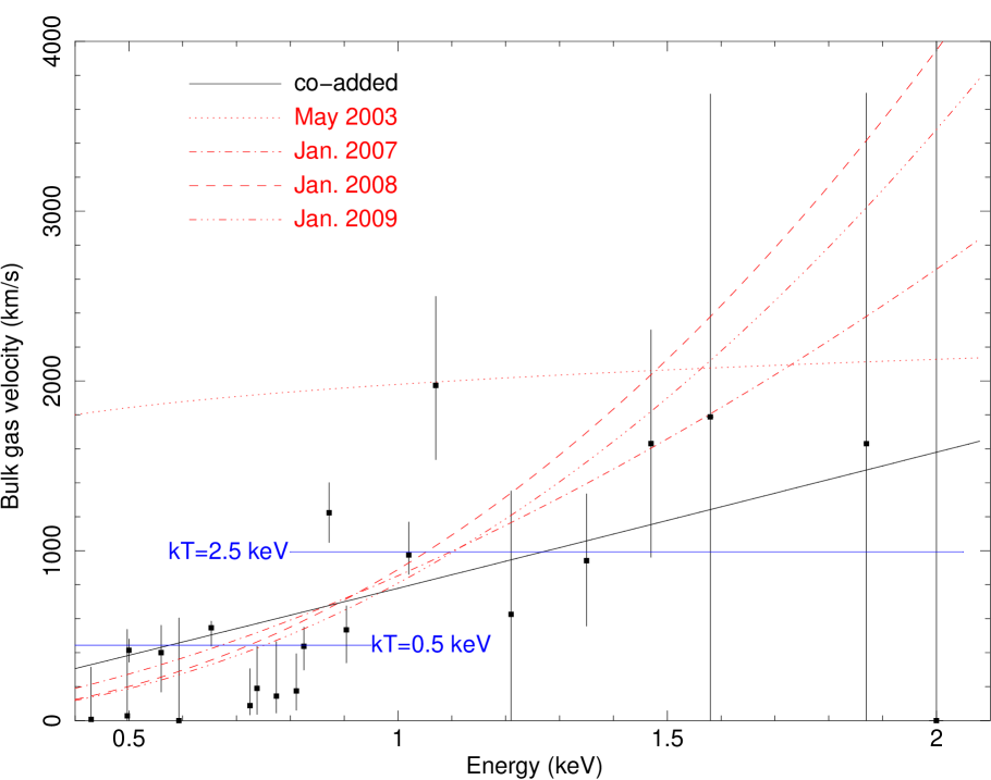
Figure 8: Squares denote the bulk gas velocity inferred from the emission line broadening derived from the Gaussian model fitted to the co-added RGS spectra. Errors are for $\Delta\chi^{2}=1$. The solid black line shows the best fit power law function to these data points. The other (red) lines show the best fit power law functions as derived with the modified vpshock model from the individual spectra. For clarity, the errors are not plotted. Note, that especially for the 2003 data the errors are large (cf. Fig. 7 right panels). The horizontal blue lines indicate the post shock gas velocities resultant from strong adiabatic shocks that heat the plasma to a temperatures of $kT=0.5$ and $2.5$ keV after thermal equilibration.

We monitored SN 1987 A with XMM-Newton and obtained RGS spectra with unprecedented statistical quality. We analyzed individual line shapes and fluxes with an empirical model and applied physical models to a combined set of RGS and EPIC-pn spectra.

The line shifts derived from the empirical model ($349\pm 24$ km s^-1) and the plasma codes ($326\pm 16$ km s^-1) are consistent. Considering the RGS wavelength scale calibration the line shifts are consistent with the systemic velocity derived from optical SN 1987 A observations (286.74$\pm$0.05 km s^-1, e.g. Gröningsson et al. 2008).

Line broadening is significantly detected in the RGS spectra. To obtain a conversion factor for the measured line widths and the bulk gas velocity, we convolved the emission spectrum of a cylindrically expanding ring at an inclination of 45°and a temperature of $kT=0.5$ keV in a bulk gas velocity range of 0 $<v_{\rm bulk}<1000$ km s^-1 with the RGS response and fitted a Gaussian to the resultant line profile. In this simulation we get v${}_{\rm bulk}=0.80\times\Delta$v (FWHM). For a similar analysis see Michael et al. (2002).

As seen in Fig. 8, v_bulk is determined best by the profiles of the two strongest lines N vii Ly_α and O viii Ly_α. The broadening of the former line including a statistical error of $\Delta\chi^{2}=2.71$ is $518_{-150}^{+130}$ km s^-1 FWHM. Since the instrumental line broadening is somewhat higher, the uncertainty of the RGS line spread function (lsf) causes a similar error. A 10% uncertainty of the lsf ($\Delta\lambda_{\rm lsf}\sim 0.07\AA\$ FWHM) gives an uncertainty range of 400$-$600 km s^-1 FWHM. But recent studies indicate that the current lsf-model rather over-estimates the instrumental line width (Jelle Kaastra, private communication). For our modeling of the RGS lines the extent of the source ($\sim$$1\aas@@fstack{\prime\prime}5$) is negligible. For a thermally equilibrated plasma, as it is expected for the shock velocity range of the lower temperature component (Rakowski 2005), the thermal line broadening also does not contribute significantly (e.g. 133 km s^-1 FWHM for nitrogen at $kT=0.5$ keV). We also found no influence due to the two unresolved Lyman transitions by modeling the line with two Gaussians, and other unresolved lines should not contribute significantly either.

For the N vii Ly_α line this indicates a bulk velocity of $(414\pm 120)$ km s^-1. In the case of gas shocked by a strong adiabatic shock wave and thermal equilibration, this yields v${}_{\rm sh}=4/3{\rm v}_{\rm bulk}=552$ km s^-1and a post shock temperature of $kT=3/16\mu{\rm v}_{\rm sh}^{2}=0.435_{-0.22}^{+0.25}$ keV. Here an adiabatic index of $\gamma=5/3$ and an average molecular weight of $\mu=0.73m_{\rm p}$ according to the abundances of the inner ring is assumed. Similarly for the O viii Ly_α line we obtain $kT=0.75_{-0.36}^{+0.22}$ keV. Thus these line widths are consistent with the temperatures derived from the plasma models.

The bulk gas velocities derived from these two lines are also consistent with the result of the Chandra LETG observation in 2007 ($\sim$360 km s^-1, Zhekov et al. 2009). But in general the bulk gas velocities as function of line energy which can be described globaly by power laws, are higher for the RGS derived values than the values deduced from the Chandra spectra (e.g. by a factor of $\sim$2 at 1 keV). Some of this difference is caused by thermal broadening, which contribute to the XMM-Newton derived line widths, but not to the Chandra values, which are based on spatial spectral deformation (i.e. the bulk gas velocity is deduced from the difference of the line broadening in the two grating arms). But this effect would only become significant for plasma out of thermal equilibrium. Also the radial velocity distribution of the shocked plasma might contribute differently to the line broadening seen in the RGS and dispersed Chandra spectra, but it can not explain such a large difference. We believe that most of the difference is caused by the different modeling methods and by calibration differences.

With our modified plasma emission code we can also investigate the evolution of the line broadening and we can narrow the artificial broadening due to blended lines. The increase in $\alpha$ indicates that the velocity of regions with lower temperature decreases relative to the regions with higher temperature. The RGS derived line widths are determined most accurately in the 0.5-1.0 keV band, where we have the best statistics and strong emission lines. Conspicuous is the sudden decrease of the line broadening in this energy band between 2003 and 2007, indicating a deceleration of the bulk velocity. Although the statistics of this observation is low, a comparison with a line broadening fixed to the function derived from the empirical model shows that the individually derived line description is significant (f-test probability $1.4\times 10^{-4}$). From 2007 to 2009 the XMM-Newton derived line widths show a rather constant line width, similar to those of the Chandra grating observations in 2004 and 2007. But from the HETG observation in 1999 Michael et al. (2002) report line widths corresponding to a post shock plasma velocity of $\sim$2500 km s^-1. Thus the line broadening had to decrease in between the XMM-Newton observation (5918 SN days) and the Chandra LETG sequence ($\sim$6400 SN days) by $\sim$50% at 1 keV. We note, that the sudden deceleration of the expansion seen in the X-ray images around day 6100 (Racusin et al. 2009) also falls into this time interval. But we emphasize that the spectra in 2003 might be more complex than assumed by two shock components and could contain a more complex mixture of radial velocity and temperature components.

Also the derived plasma parameters of the plasma emission model show a clear evolution between 2003 and 2007. The emission measure ratio $EM_{2}/EM_{1}$ shows a decrease. During this time also the soft flux was rising drastically. In the later observations the $EM$ ratio is rather constant with a tendency of an increase.

We also observe the ongoing ionization of the plasma. This causes e.g. the increase of the [Ne x Ly_α]/[Ne ix He r] flux ratio by $\sim$26% during the last two observations. The upper limit of the ionization timescale range $\tau_{\rm u}$ is steadily increasing for both plasma components. $\tau_{\rm u,1}$ indicates some upturn after the first observation, which could be caused by an increasing density. A fit of a linear function to the last three values (see Fig. 7) yields an ”average” density of $n_{1}=(3.24\pm 0.64)$$\times 10^{3}$ cm^-3. For the high temperature component no evolution in density is observed and a similar fit yields $n_{2}=(4.8\pm 1.4)$$\times 10^{2}$ cm^-3. The ratio of the emission measure of the low and high temperature components is roughly constant with a volume ratio of $\sim$7.5.

The densities derived from the unshocked gas in the optical are $6\times 10^{3}$ cm${}^{-3}<n<3\times 10^{4}$ cm^-3 for the ring and $\sim$$10^{2}$ cm^-3 for the extended nebula (Lundqvist & Fransson 1996). A strong adiabatic shock wave increases these densities by a factor of four. Our values would suggest less denser regions in the ring and the surrounding nebula as origin of the X-rays. But the vpshock model assumes a ionization time distribution linear in emission measure, which is clearly not true for SN 1987 A. A complex density distribution and effects of radial expansion affect the derived densities. However, these values are not consistent with those from the modeling of the light curve (Haberl et al. 2006; Aschenbach 2007), and should be regarded with some care.

The temperature of the soft plasma component shows a strong increase between the first two observations, and a slight increase in the later ones. Also from Chandra observations a rising temperature of this component is derived (Park et al. 2006). Between 2004 and 2007 Zhekov et al. (2009) report a nearly constant temperature. With RGS we can see an ongoing small increase in the temperature of the soft component. However, a decrease caused by the deceleration of the shock wave and adiabatic expansion of the shocked plasma is expected which is seen in the high temperature component. An increase is possible, if regions with slightly higher temperature contribute more to the emission measure with time, e.g. due to more rapidly rising volume of these regions. But also the effects of incomplete thermal equilibration might contribute to a rising electron temperature, especially initially after the shock wave has reached denser protrusions of the ring.

The abundances derived from the two component plan-parallel shock model (cf. Table 4) are higher (on average by a factor of 1.8), than derived by Heng et al. (2008, VPSHOCK+VPSHOCK W00 model). Heng et al. used a similar model, but fitted only the EPIC-pn spectum of the 2007 observation and derived different plasma parameters (e.g. temperatures) which influences the derived abundances. Compared with the Chandra grating results of Zhekov et al. (2009), our abundances are consistent within 30%, except nitrogen, where our value is higher (by a factor of 1.7) but rather matches the Lundqvist & Fransson (1996) value, and Mg and Fe, which are $\sim$30% lower. We see, that the individual modelling causes systematic differences, much larger than the statistical errors. We also note, that the abundances derived from the plane-parallel shock model are lower than the abundances of the inner ring as derived from Lundqvist & Fransson (1996), whereas the abundances of the sedov+powerlaw model are higher. Thus the lower abundances derived so far in X-ray analysis may be caused by the assumption of a two component plan-parallel shock structure.

As shown in the right panel of Fig. 4, we see a clear indication for an Fe K feature. The black curve in Fig. 4 shows the emission from the shocked plasma of the inner ring, as expected from our two component shock model, which describes the Fe L lines well. Surprisingly we find, that the feature suggests a contribution of emission at lower energy of less ionized, or even neutral, iron as it is present in the unshocked part of the ring and in the supernova debris. In the case of a very young ($\tau_{\rm u}\leq 3\times 10^{10}$) reverse shock in a iron rich region, we would also expect emission from other elements in the RGS spectra. If the additional emission is caused by fluorescence (6.4 keV), this would need neutral iron. In this case, the iron could be excited by X-rays from the shocked ring, but this would need a much higher column density of the unshocked region. Thus the emission might originate from the supernova debris, where a higher column density is possible and reprocessed radiation from nuclear decays might contribute.

5 Conclusions

1. With our monitoring we can follow the detailed evolution of the supernova remnant of SN 1987 A. E.g. the upturn in ionization age and emission measure ratio between 2003 and 2007 shows that the blast wave was propagating into the inner ring.

2. The decreasing line widths at lower energies in between the first two observations indicate a deceleration of the lower temperature plasma, that correlates well with the decelerating ring expansion as observed in the Chandra images.

3. The electron temperature derived for the soft temperature component with plasma models is consistent with the line widths of the emission lines in the corresponding energy range. This is expected, if the emission is primary caused by shocks transmitted into denser regions.

4. The lower statistics at higher energies do not justify such conclusions for the high temperature component, where the bulk velocity can be reduced by the contribution of reflected shocks which would also heat the plasma further. But the decreasing temperature with time and the higher line widths seen by XMM-Newton and Chandra rather suggest forward shocks in less denser regions as the dominating process.

5. The iron K feature argues rather for a thermal high energy component and little if any non-thermal contribution. The line shape further suggests the contribution ($\sim$50%) of a cold iron line (2.3$\sigma$ level), possibly emitted from the supernova debris.

Further monitoring will yield information on the arising SNR of SN 1987 A and the increasing statistics of the brightening source will allow even more detailed analyses also beyond the assumption of plane-parallel geometry. This might put further constraints on the origin of the X-ray emitting regions and their dynamics. Similarly the iron K emission can yield information on the evolution of the debris.

References

- Anders & Grevesse (1989) Anders, E. & Grevesse, N. 1989, Geochim. Cosmochim. Acta., 53, 197
- Arnaud (1996) Arnaud, K. A. 1996, in Astronomical Society of the Pacific Conference Series, Vol. 101, Astronomical Data Analysis Software and Systems V, ed. G. H. Jacoby & J. Barnes, 17
- Aschenbach (2007) Aschenbach, B. 2007, in American Institute of Physics Conference Series, Vol. 937, Supernova 1987A: 20 Years After: Supernovae and Gamma-Ray Bursters, ed. S. Immler, K. Weiler, & R. McCray, 33–42
- Beuermann et al. (1994) Beuermann, K., Brandt, S., & Pietsch, W. 1994, A&A, 281, L45
- Borkowski et al. (2001) Borkowski, K. J., Lyerly, W. J., & Reynolds, S. P. 2001, ApJ, 548, 820
- den Herder et al. (2001) den Herder, J. W., Brinkman, A. C., Kahn, S. M., et al. 2001, A&A, 365, L7
- Dewey et al. (2008) Dewey, D., Zhekov, S. A., McCray, R., & Canizares, C. R. 2008, ApJ, 676, L131
- Gaensler et al. (2007) Gaensler, B. M., Staveley-Smith, L., Manchester, R. N., et al. 2007, in American Institute of Physics Conference Series, Vol. 937, Supernova 1987A: 20 Years After: Supernovae and Gamma-Ray Bursters, ed. S. Immler, K. Weiler, & R. McCray, 86–95
- Gröningsson et al. (2008) Gröningsson, P., Fransson, C., Leibundgut, B., et al. 2008, A&A, 492, 481
- Gröningsson et al. (2006) Gröningsson, P., Fransson, C., Lundqvist, P., et al. 2006, A&A, 456, 581
- Haberl et al. (2006) Haberl, F., Geppert, U., Aschenbach, B., & Hasinger, G. 2006, A&A, 460, 811
- Hasinger et al. (1996) Hasinger, G., Aschenbach, B., & Truemper, J. 1996, A&A, 312, L9
- Heng et al. (2008) Heng, K., Haberl, F., Aschenbach, B., & Hasinger, G. 2008, ApJ, 676, 361
- Heng et al. (2006) Heng, K., McCray, R., Zhekov, S. A., et al. 2006, ApJ, 644, 959
- Hughes et al. (1998) Hughes, J. P., Hayashi, I., & Koyama, K. 1998, ApJ, 505, 732
- Jansen et al. (2001) Jansen, F., Lumb, D., Altieri, B., et al. 2001, A&A, 365, L1
- Lawrence et al. (2000) Lawrence, S. S., Sugerman, B. E., Bouchet, P., et al. 2000, ApJ, 537, L123
- Lundqvist & Fransson (1996) Lundqvist, P. & Fransson, C. 1996, ApJ, 464, 924
- McCray (2007) McCray, R. 2007, in American Institute of Physics Conference Series, Vol. 937, Supernova 1987A: 20 Years After: Supernovae and Gamma-Ray Bursters, ed. S. Immler, K. Weiler, & R. McCray, 3–14
- Michael et al. (2003) Michael, E., McCray, R., Chevalier, R., et al. 2003, ApJ, 593, 809
- Michael et al. (2002) Michael, E., Zhekov, S., McCray, R., et al. 2002, ApJ, 574, 166
- Ng et al. (2008) Ng, C.-Y., Gaensler, B. M., Staveley-Smith, L., et al. 2008, ApJ, 684, 481
- Park et al. (2006) Park, S., Zhekov, S. A., Burrows, D. N., et al. 2006, ApJ, 646, 1001
- Park et al. (2005) Park, S., Zhekov, S. A., Burrows, D. N., & McCray, R. 2005, ApJ, 634, L73
- Plucinsky et al. (2008) Plucinsky, P. P., Haberl, F., Dewey, D., et al. 2008, in Society of Photo-Optical Instrumentation Engineers (SPIE) Conference Series, Vol. 7011, Society of Photo-Optical Instrumentation Engineers (SPIE) Conference Series
- Racusin et al. (2009) Racusin, J. L., Park, S., Zhekov, S., et al. 2009, ApJ, 703, 1752
- Rakowski (2005) Rakowski, C. E. 2005, Advances in Space Research, 35, 1017
- Strüder et al. (2001) Strüder, L., Briel, U., Dennerl, K., et al. 2001, A&A, 365, L18
- Sturm et al. (2009) Sturm, R., Haberl, F., Hasinger, G., Kenzaki, K., & Itoh, M. 2009, PASJ, 61, 895
- Turtle et al. (1990) Turtle, A. J., Campbell-Wilson, D., Manchester, R. N., Staveley-Smith, L., & Kesteven, M. J. 1990, IAU Circ., 5086, 2
- Wilms et al. (2000) Wilms, J., Allen, A., & McCray, R. 2000, ApJ, 542, 914
- Zhekov et al. (2005) Zhekov, S. A., McCray, R., Borkowski, K. J., Burrows, D. N., & Park, S. 2005, ApJ, 628, L127
- Zhekov et al. (2006) Zhekov, S. A., McCray, R., Borkowski, K. J., Burrows, D. N., & Park, S. 2006, ApJ, 645, 293
- Zhekov et al. (2009) Zhekov, S. A., McCray, R., Dewey, D., et al. 2009, ApJ, 692, 1190