Measuring the Speed of Dark: Detecting Dark Energy Perturbations
Abstract
The nature of dark energy can be probed not only through its equation of state, but also through its microphysics, characterized by the sound speed of perturbations to the dark energy density and pressure. As the sound speed drops below the speed of light, dark energy inhomogeneities increase, affecting both CMB and matter power spectra. We show that current data can put no significant constraints on the value of the sound speed when dark energy is purely a recent phenomenon, but can begin to show more interesting results for early dark energy models. For example, the best fit model for current data has a slight preference for dynamics (), degrees of freedom distinct from quintessence (), and early presence of dark energy (). Future data may open a new window on dark energy by measuring its spatial as well as time variation.
I Introduction
Although dark energy dominates the energy density of the universe and drives the accelerating cosmic expansion, we know remarkably little about it. Over the course of the past decade, cosmologists have devoted considerable effort to devising new and sharpening known methods for determining the equation of state of dark energy. The equation of state, defined as the pressure to energy density ratio, is generally a time dependent function and fully specifies the temporal evolution of dark energy density. The dark energy density in turn (along with the matter density) determines the expansion rate of the universe, as well as geometrical measures (distances and volumes).
The equation of state does not, however, tell us about the microphysics of dark energy, nor does it describe all of the cosmological signatures. For example, even a perfectly measured does not tell us whether dark energy arises from a canonical, minimally coupled scalar field, a more complicated fluid description, or modification of gravitational theory on large scales. The properties of the perturbations to the dark energy, which must exist unless it is simply a cosmological constant or only an effective field, do carry such extra information.
Perturbations to the energy density and pressure can be described through the sound speed, . The sound speed carries information about the internal degrees of freedom: for example, rolling scalar fields (quintessence) necessarily have sound speed equal to the speed of light, . Detection of a sound speed distinct from the speed of light would indicate further degrees beyond a canonical, minimally coupled scalar field.
A low sound speed enhances the spatial variations of the dark energy, giving inhomogeneities or clustering. Heuristically, the sound speed determines the sound horizon of the fluid, , where is the Hubble scale. On scales below this sound horizon, the fluid is smooth; on scales above , the fluid can cluster. Since for quintessence , the sound horizon equals the cosmic horizon size and there are essentially no observable inhomogeneities. However, if the sound speed is smaller, then dark energy perturbations may be detectable on correspondingly more observable (though typically still large) scales. These perturbations act in turn as a source for the gravitational potential, and affect the propagation of photons. For example, clustering dark energy influences the growth of density fluctuations in the matter, and large scale structure, and an evolving gravitational potential generates the Integrated Sachs-Wolfe (ISW) effect Sachs and Wolfe (1967) in the cosmic microwave background. The observational signatures of these effects offer a way of probing the dark energy inhomogeneity and sound speed.
In this paper we study the signatures of the sound speed of dark energy. We revisit and extend previous studies of dark energy clustering Hu et al. (1999); Hu (2002); Erickson et al. (2002); DeDeo et al. (2003); Weller and Lewis (2003); Bean and Dore (2004); Afshordi (2004); Hu and Scranton (2004); Hannestad (2005); Corasaniti et al. (2005); Koivisto and Mota (2006); Takada (2006); Xia et al. (2008); Ichiki and Takahashi (2007); Mota et al. (2007); Bashinsky (2007); Torres-Rodríguez et al. (2008); Dent et al. (2009); Ballesteros and Riotto (2008); Sapone and Kunz (2009), clarifying and quantifying the physical effects caused by the nonstandard values for the speed of sound. We then study models where the dark energy density was non-negligible at early times, which offer much better prospects for observable signatures than the fiducial near-CDM case. Finally, using current cosmological data, we constrain the speed of sound jointly with 7-8 other standard cosmological parameters.
This paper is organized as follows. In Sec. II we describe dark energy perturbations and the physical influence of the sound speed and equation of state, deriving the dark energy density power spectrum. Section III describes the dark energy models we consider, and Sec. IV treats the impact of dark energy inhomogeneity on the CMB, matter power spectrum, and their crosscorrelation. We consider models with both constant and time varying equation of state and sound speed in Sec. V, and present constraints from current data.
II Dark Energy Perturbations
We briefly review the growth of density perturbations, in both the matter and dark energy, focusing on the role of the sound speed. See Kodama and Sasaki (1984); Ma and Bertschinger (1995) for more details. To derive the influence of the sound speed on dark energy inhomogeneity, and dark energy perturbations on the matter distribution, we must solve the perturbed Einstein equations for the density perturbations , pressure perturbations , and velocity (divergence) perturbations . We do not consider an anisotropic stress.
In the conformal Newtonian gauge, the perturbed Friedmann-Robertson-Walker metric takes the form
| (1) |
where is the scale factor, is the conformal time, represents the three spatial coordinates, and and are the metric potentials. Conservation of the stress-energy tensor () of a perfect fluid gives the following equations in Fourier space (see, e.g., Ma and Bertschinger (1995)) from the time-time and space-space parts:
| (2) | |||||
where is the wavevector, dots are derivatives with respect to conformal time, is the conformal Hubble parameter, is the density perturbation, is the velocity perturbation, and is the equation of state. These equations hold for each individual component, i.e. matter or dark energy.
We define the effective (or rest frame) sound speed through (see, e.g., Hu (1998))
| (3) |
where the adiabatic sound speed squared is
| (4) |
In terms of , Eqs. (2) and (II) read
| (6) |
One can readily see that the source term in a equation will have a negative term involving from (take the derivative of Eq. II and substitute in Eq. 6), indicating that growth is suppressed on small scales, . However, perturbations will exist in the dark energy density even for , albeit at a very low level within the Hubble scale . As drops below unity, the suppression is itself suppressed and inhomogeneities in the dark energy can be sustained. All such perturbations will vanish though as , regardless of . In the combination of Eqs. (II) and (6) into a single second order equation for , the terms involving the metric in this equation are all proportional to (or derivatives thereof) so that in the limit the perturbations decouple from the metric and do not experience a gravitational force leading to growth.
The dark energy perturbations affect the metric perturbations, and thus the perturbations in the matter, through the Poisson equation
| (7) |
where the sum runs over all components. For a perfect fluid, there is no anisotropic stress so .
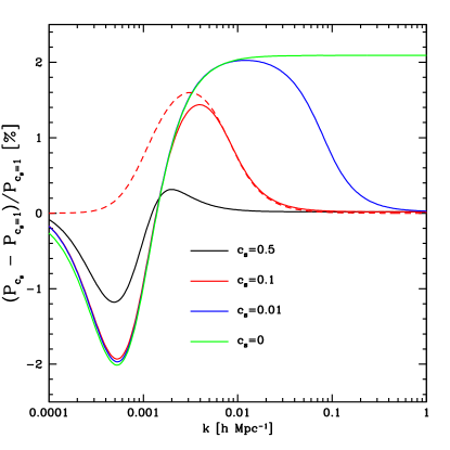
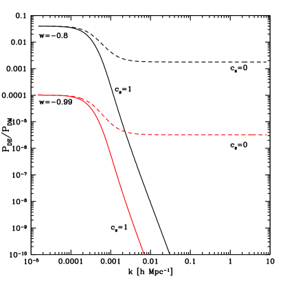
Therefore we expect the density power spectrum to be affected by the dark energy sound speed in distinct ways on different scales. On superhorizon scales, , the density power spectrum becomes independent of the dark energy sound speed. Here the perturbations are determined by the curvature fluctuation Bardeen (1980); Bertschinger (2006). Between the Hubble scale and the sound horizon, , a sound speed will enhance the density inhomogeneities (modulo gauge dependence around the Hubble scale). Finally, on smaller scales, , inhomogeneity growth is always suppressed and the sound speed becomes irrelevant. We illustrate these behaviors in Figure 1. (All power spectra in this paper are for linear theory and shown at , and are calculated using CAMB Lewis et al. (2000) and CMBeasy Doran and Müller (2004); Doran (2005).) Note that the strength of the deviation from the behavior is a steep function of for .
III Dark Energy Models
We study three classes of dark energy models to elucidate the role of sound speed and , from early to late times.
1) Constant models. We begin with the simplest model of dark energy with sound speed different from the speed of light: a constant equation of state and a constant sound speed . This is mostly for historical comparison to Bean and Dore (2004), since the current constraint on constant equation of state is Amanullah et al. (2007) (using only geometric data independent of the sound speed) and so the effects of sound speed are suppressed due to .
2) Early dark energy with constant speed of sound (cEDE). In order to allow for a period where is further from and so the sound speed has more influence, we also consider a model with varying equation of state but constant sound speed. We choose the phenomenological early dark energy model of Doran and Robbers (2006) but allow to be a free (constant) parameter. At early times approaches 0 in this model and so the value of can have observational consequences. The model parameters are the fraction of dark energy density at early times (this approaches a constant), the equation of state today , and . We call this generalization the cEDE model. Here
| (8) | |||||
| (9) |
where the current dark energy density . In this model, . We show an example of in Figure 2.
3) Barotropic (“aether”) dark energy models. The third model we treat is a particular case of the barotropic class of dark energy, where there is an explicit relation determining the pressure as a function of energy density. Several physical models for the origin of dark energy fall in this class, and have attractive properties as discussed below.
Ref. Linder and Scherrer (2009) showed that all such viable models could be written as a sum of an asymptotic constant energy density (with ) and a barotropic fluid, or aether, with positive equation of state . The sound speed is completely determined by and has the property that . Moreover, to admit an early matter dominated era, , and hence . We adopt the form so
| (10) | |||||
| (11) | |||||
| (12) | |||||
| (13) |
where . There are two free parameters in addition to the dark energy density today: and – one less than in the cEDE case (we will fix usually). Note that the effective early dark energy density and the present equation of state is . As discussed by Linder and Scherrer (2009), the barotropic model strongly ameliorates the coincidence problem, motivating why today.
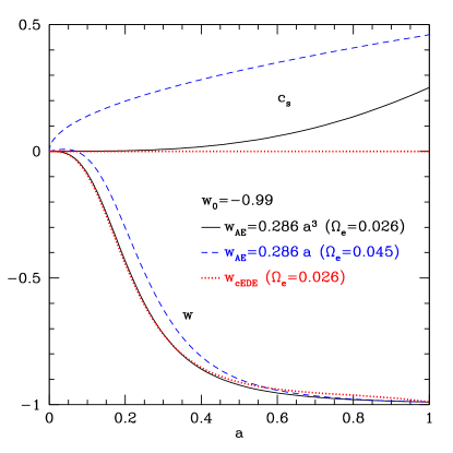
Our three models thus span constant and constant , varying and constant , and varying and varying (but with determined by ). We illustrate their equation of state and sound speed behaviors in Figure 2. We expect a cEDE early dark energy model with to show the greatest effect of sound speed on the observables. Since cEDE can look so much like the barotropic model, in and more approximately in , we do not treat the barotropic model separately in the following sections, but rather consider it as a motivation for cEDE. The barotropic model possesses the advantage of having at early times (and at late times) being determined by physics rather than being adopted as phenomenology.
IV Impact on Cosmological Observations
We now consider angular power spectra of cosmological observables that are sensitive to the speed of sound of dark energy, with the aim of comparing the predictions to current observations (so we do not here include higher order correlations, leaving for future work such signatures and their effect on constraining non-Gaussianity).
IV.1 Angular Power Spectra
The matter density fluctuations, potential fluctuations, and the radiation field are influenced by the dark energy sound speed as discussed in Sec. II. From these we can form, and measure, the angular auto- and cross-power spectra. We consider the CMB temperature anisotropy power spectrum, the galaxy (or other large scale structure tracer) overdensity field in a redshift bin , and their crosscorrelation, giving the power spectra , where . See the Appendix for a review of how the power spectra relate to the potential power spectrum.
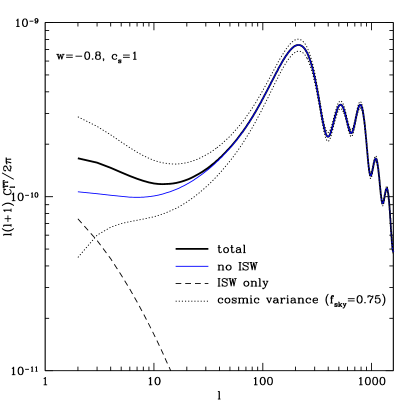
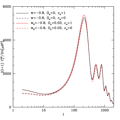
Figure 3 shows a typical temperature power spectrum. The signal from the sound speed dependence enters through the ISW effect, which is also plotted separately in the figure. The extra power from the ISW effect arises from the decay of the potential as the dark energy impacts matter domination at late times; in the concordance model the cosmological constant dark energy causes a decay in the potentials of about between the matter dominated era and the present. While the decay arises from the change in the expansion history due to the dark energy equation of state, it can be ameliorated by increased dark energy clustering if the dark energy sound speed is small. Figure 4 illustrates the influence of the sound speed.
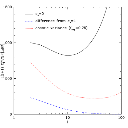
The ISW effect can be measured Boughn and Crittenden (2004); Nolta et al. (2004); Fosalba et al. (2003); Scranton et al. (2003); Fosalba and Gaztañaga (2004); Padmanabhan et al. (2005); Afshordi et al. (2004); Cabre et al. (2006); Ho et al. (2008); Giannantonio et al. (2008) and one might hope to constrain the sound speed in this way. However, since the effect occurs only on the largest angular scales, cosmic variance swamps the signal. This is demonstrated in the left panel of Fig. 4 for a cosmic variance limited experiment scanning 3/4 of the whole sky. The right panel explicitly displays the low signal-to-noise for each multipole, with the difference between and only amounting to when summed over all multipoles.

For the galaxy or matter density fluctuations, the dark energy sound speed can have a larger effect. Note that the dark energy perturbations themselves remain small relative to the matter inhomogeneities, despite a low sound speed having a dramatic effect on the dark energy clustering. Figure 5 shows that on superhorizon scales the level of dark energy power is relative to the dark matter power (because at superhorizon scales the perturbations remain adiabatic and the ratio ). On subhorizon scales, the ratio depends strongly on the dark energy sound speed. For , the ratio is scale independent in the subhorizon regime: during matter domination, one can show analytically that then
| (14) |
but this ratio becomes smaller by roughly a factor of two by today. For a canonical sound speed , the dark energy power is strongly suppressed relative to the dark matter power, with the ratio scaling as .
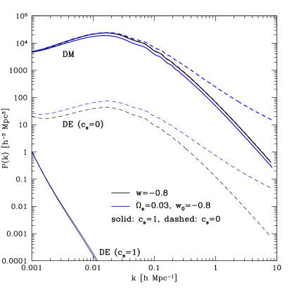
The matter power spectrum itself, however, is affected by the dark energy sound speed through the potential perturbations induced by the dark energy inhomogeneities. Figure 6 shows in the left panel the absolute comparison of the dark matter and dark energy power (in contrast to the relative difference between the two in Fig. 5). On this log scale one cannot see the influence of the dark energy sound speed on the dark matter power, so the right panel plots the deviation with respect to the case. We see that the deviation due to is at the percent level in the matter density power and the tens of percent level in the potential perturbation power.
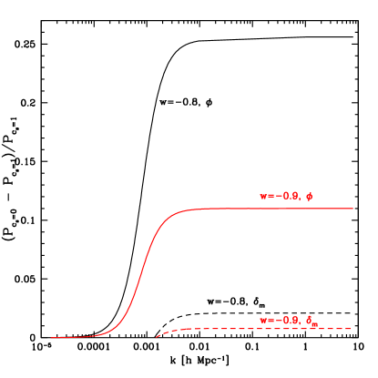
The density and potential are related through the Poisson equation. For example, for and , the amplitude of the dark energy perturbations is about of the dark matter perturbation (i.e. the power ratio is about on subhorizon scales as seen from Fig. 5). According to the Poisson equation, Eq. (7), this translates into about a increase in going from to , because today and because in the case the dark energy contribution to the Poisson equation is negligible. Hence, as shown in the right panel of Fig 6, we get about a increase in the power spectrum of .
Note that the (late) ISW effect is proportional to the change in potential between matter domination and today. In the standard case, this decay is about of the potential during matter domination and thus about of the potential today, i.e. . Hence, the change in the potential at present of due to enhanced dark energy clustering corresponds to a change in the ISW effect of approximately (i.e. in . This enhancement gives the ISW effect extra sensitivity to dark energy clustering relative to other probes.
The matter density perturbation is of course also affected, but with only about a increase in its amplitude. This effect on the potential today through the Poisson equation is therefore subdominant to the direct effect of the dark energy perturbation itself.
Now that we have seen the basic effects of the dark energy sound speed and equation of state on the observables, we consider the specific instances of the constant model and cEDE model. We can already guess that to obtain reasonable constraint on the sound speed we will want a model that has as large a and as small a as is consistent with the observations, for a substantial part of cosmic history.

IV.2 Estimating constraints in constant Model
We begin by estimating the chances of constraining the sound speed using the between two extremes: and . Since we consider angular power spectra and crosscorrelations of observables on the sky (labeled by capital letters below), is in general given by
| (15) |
where is the difference in spectra between the two cases and the covariance is given by
| (16) |
with
| (17) |
where is the fraction of the sky that is observed, are the fiducial spectra and are the noise power spectra so that are the observed power spectra that include the noise. (See the Appendix for further details.) For the estimates of this section we only consider the CMB temperature power spectrum and we will consider the cosmic variance dominated limit where the noise power spectrum is much smaller than the fiducial power spectrum, . Hence, Eq. (15) simplifies to
| (18) |
Assuming Gaussian likelihood, the quantity is equivalent to the signal to noise squared with which we can distinguish from our fiducial if all the other parameters were known exactly. Since in reality we should marginalize over the other parameters as well, is an upper bound on the signal to noise squared for distinguishing the two sound speeds. Therefore if we find a low then there is little hope of constraining with the assumed dataset. To amplify the chances of detection, we examine , since in the limit dark energy perturbations become irrelevant regardless of the value of the value of the sound speed; given that is already an unlikely value given current data, the calculated signal to noise squared could be an overoptimistic estimate of the true value.
Figure 4 confirms that the discrimination between sound speeds through the CMB temperature autocorrelation is poor, as discussed in the previous subsection. Cosmic variance swamps the difference between even the extremes, and , and the total . Note that this took cosmic variance to be calculated from the most optimistic case, , where the noise is significantly lower, so one truly cannot determine with the CMB temperature anisotropy despite all the most optimistic assumptions.
The overall significance of the mere existence of the ISW effect (i.e. the between the CMB power with the ISW effect artificially removed and the true CMB) is only . The potential decay in a model with dark energy sound speed is a little less than half the contribution in the case, thus explaining the quoted above. Thus the ISW signal in the CMB temperature spectrum is too blunt a tool to explore dark energy sound speed.
We must go beyond the CMB temperature spectrum to consider the galaxy-galaxy power and temperature-galaxy crosscorrelation data. Rather than proceeding further with halfway measures such as calculating the signal to noise to determine whether we would be able to place to constraints on while fixing all other parameters, we instead carry out a full likelihood analysis in Sec. V.
IV.3 Estimating constraints in cEDE model
In the early dark energy case, we find that the ISW signal in both the CMB temperature autocorrelation and temperature-galaxy crosscorrelation is comparable to the signal in the case of ordinary dark energy (which typically has an energy density fraction relative to matter of at CMB last scattering). However, there is another source of distinction. Dark energy in the cEDE model has at CMB last scattering; if in addition , then cEDE behaves at early times just like dark matter, with significant clustering of the dark energy. This will affect not only the large scale, late time ISW contribution to the CMB but also the early Sachs-Wolfe effect and the acoustic peaks.
Therefore we expect a clearer observational signature of the sound speed than for ordinary dark energy. Figure 7 shows the effect of changing the sound speed in the cEDE model. The CMB temperature autocorrelation alone delivers (for ). This seems more promising for constraining the sound speed, and again we proceed to a full likelihood analysis.
V Measuring the Speed of Darkness
To obtain accurate constraints on the dark energy sound speed we perform a Markov Chain Monte Carlo (MCMC) likelihood analysis over the set of parameters , where is either , in the constant case, or , in the cEDE case, is the present physical baryonic energy density density, is the present physical cold dark matter energy density, is the present relative energy density in the dark energy, is the reionization optical depth, the amplitude of primordial scalar perturbations (defined relative to a pivot scale of ) and is the spectral index of the primordial scalar perturbations. Note that we choose as the sound speed parameter because most of the sensitivity is at small values of .
For current data we include the CMB temperature power spectrum from WMAP5 Komatsu et al. (2009), the crosscorrelation of these temperature anisotropies with mass density tracers including the 2MASS (2-Micron All Sky Survey), SDSS LRG (Sloan Digital Sky Survey Luminous Red Galaxies), SDSS quasars, and NVSS (NRAO VLA All Sky Survey) radio sources, following Ho et al. (2008), and the SDSS LRG autocorrelation function from Tegmark et al. (2006). To break degeneracies with background cosmology parameters and constrain the expansion history, we use the supernovae magnitude-redshift data from the Union2 compilation Amanullah et al. (2007).
The MCMC package COSMOMC Lewis and Bridle (2002) is used to calculate the joint and marginalized likelihoods. The results for the marginalized 1D probability distributions are shown in Fig. 8 for the constant equation of state case and in Fig. 9 for the early dark energy, cEDE case. Dotted lines show the distributions when one fixes .


In the constant case, no constraint can be placed on the sound speed, as expected from our earlier arguments. In addition, the other parameter distributions are essentially unaffected by the value of . For the cEDE case, however, some preference appears for a low sound speed, , and this propagates through to the other parameters. Since early dark energy with a low sound speed acts like additional dark matter at early times, this allows a lower true matter density.
It is intriguing to consider whether the apparent preference of current data for the CDM model is merely a consequence of overly restricting the degrees of freedom of dark energy, and that instead a dark energy with dynamics (), microphysics (), and long-time presence () could be the correct model.
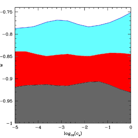
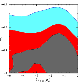
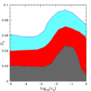
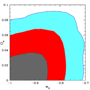
Figure 10 shows the 68.3%, 95.4% and 99.7% confidence level contours in the - plane for the constant model. We see that current data in this model prefer but are completely agnostic regarding . For the cEDE model, Fig. 11 shows the joint probability contours among the dark energy parameters, in the -, -, and - planes, with all other parameters marginalized. Here we see that the model mentioned above, , is completely consistent with the data, as is the cosmological constant . It will be interesting to see how the best fit evolves with future data.
VI Conclusions
Current cosmological data are in excellent agreement with the standard CDM universe, with equation of state . Nevertheless, the current data are also consistent with a wide variety of richer physics. It is not clear that it is wise to assume that the physical explanation for dark energy in the universe is indeed given by restriction to a spatially smooth, constant in time energy density: the cosmological constant. Even after allowing for dynamical dark energy, there could be further degrees of freedom – “hidden variables” or microphysics – in the dark energy sector, harbingers of deeper physics that have not yet shown clear signatures in the data. An explicit search for these signatures, and thus the physics behind dark energy, should be near the top of the list of current efforts in cosmology.
In this paper we search for degrees of freedom beyond quintessence by examining the influence of the sound speed of dark energy, and its resulting spatial clustering of dark energy, on key observables and in current data. This extends earlier analyses, quantifying the effects on the dark matter and dark energy density perturbation power spectra, the potential power spectrum, and their crosscorrelation. Where possible, we give simple scalings with and . We also explore models with time varying equation of state and sound speed.
In the standard model with negligible dark energy at high redshift, the speed of sound is essentially not distinguishable with current data (see Fig. 8) because current data favor , and the effects of clustering of dark energy vanish in this limit. As gets further from , the influence of the sound speed increases; for models with at high redshift there is also the possibility of non-negligible amounts of early dark energy density. Even just a couple percent of the total energy density in early dark energy dramatically improves the prospects for detecting dark energy clustering. One can view the early dark energy fraction as another degree of freedom to explore. Indeed, carrying out a MCMC analysis we find in Figs. 9 and 11 that a model with dynamics, microphysics, and persistence: is completely consistent with the current data (although remains consistent as well).
Discovery of the accelerating universe 12 years ago has propelled the physical interpretation of dark energy into one of the most important, exciting, and difficult problems in physics. Although current observations indicate that the equation of state, as a constant or broadly averaged over time, is close to , this leaves considerable room for further physics, as demonstrated here using recent data. To go further we should explore all three frontiers of the dynamics , the microphysics and spatial inhomogeneities, and the persistence .
Acknowledgements.
We are extremely grateful to the Supernova Cosmology Project for permission to use the Union2 supernova data before publication and for use of their computer cluster. RdP thanks Jeff Anderson for invaluable computer support and Marina Cortês for useful conversations about MCMC. EL and RdP have been supported in part by the Director, Office of Science, Office of High Energy Physics, of the U.S. Department of Energy under Contract No. DE-AC02-05CH11231, and EL by the World Class University grant R32-2008-000-10130-0. DH is supported by the DOE OJI grant under contract DE-FG02-95ER40899, NSF under contract AST-0807564, and NASA under contract NNX09AC89G.Appendix A Angular Power Spectra: Definitions
Here we review how the observable power spectra of various quantities on the sky are related to the three-dimensional primordial power spectrum and the transfer functions. We consider the CMB temperature anisotropies and galaxy overdensities in redshift slices, or populations, labeled with the subscript , and write the observables in direction as line of sight projections along comoving radial coordinate ,
| (19) |
with the “source term” as a function of comoving position and conformal time ( is the age of the universe in conformal time). Here represents the observable, which could be a galaxy overdensity in the th redshift bin or a CMB temperature anisotropy . For the galaxy overdensity , the source is
| (20) |
where is the average angular galaxy density of galaxy population in the redshift interval , is the total average angular galaxy density of population , and is the galaxy bias relative to the matter overdensity of bin . The Hubble factor arises because the source was defined in terms of an integral over while is normalized to unity in terms of an integral over .
For CMB temperature anisotropies, the (Fourier transform of the) source is given in Eq. (12) of Seljak and Zaldarriaga (1996). The Integrated Sachs-Wolfe contribution to the CMB anisotropy is nonzero when the universe is not matter dominated, and thus the gravitational potentials and are not constant. The ISW source is given by
| (21) |
where dots denote derivatives with respect to conformal time.
If we expand the anisotropy field in spherical harmonics, , the expansion coefficients are given by
| (22) | |||||
where we have Fourier expanded
| (23) |
and we have used the Rayleigh plane-wave expansion
| (24) |
where the is the spherical Bessel function. We now write where is the initial potential perturbation and is the source for , i.e. it is a transfer function. Due to the assumption of homogeneity, the transfer function does not depend on the direction of the wavenumber, but only on its magnitude . The statistics of the initial perturbations are given by
| (25) |
where is the primordial potential power spectrum. Assuming statistical isotropy, the angular correlations between two quantities on the sky and (where they may or may not be the same) is given by the angular power spectrum
| (26) |
where, using Eq. (22),
| (27) | |||||
In this work, we are specifically interested in the combinations , but Eq. (27) is the general expression for angular power or crosscorrelation spectra.
When the sources and vary slowly compared to the spherical Bessel functions in Eq. (27), the triple integral can to a good approximation be reduced to a single integral. Setting and using the asymptotic (for ) formula that , we find
| (28) | |||||
where . We use the power spectra to calculate the (signal-to-noise) in Eq. (15).
Finally, we need to specify formulae for noise in the observed spectra . The covariances between the spectra are given by
| (29) |
where
| (30) |
Here is the sky coverage, are the fiducial spectra and are the noise power spectra. For the galaxy density fields, the white noise power spectra are given by
| (31) |
and for the CMB it is given by
| (32) |
where is the sensitivity and is the full width half max angle of the Gaussian beam. The noise cross power spectra can be assumed to vanish.
The treatment of the covariances for actual data is typically more complicated than the above. In this paper, we use the covariances and treatment of the observables as given by the data packages in COSMOMC, Ho et al. (2008); Tegmark et al. (2006); Komatsu et al. (2009) for the angular spectra, and the Union2 supernovae covariance matrix including systematics.
References
- Sachs and Wolfe (1967) R. K. Sachs and A. M. Wolfe, Astrophys. J. 147, 73 (1967).
- Hu et al. (1999) W. Hu, D. J. Eisenstein, M. Tegmark, and M. J. White, Phys. Rev. D59, 023512 (1999), eprint arXiv:astro-ph/9806362.
- Hu (2002) W. Hu, Phys. Rev. D65, 023003 (2002), eprint arXiv:astro-ph/0108090.
- Erickson et al. (2002) J. K. Erickson, R. R. Caldwell, P. J. Steinhardt, C. Armendariz-Picon, and V. F. Mukhanov, Phys. Rev. Lett. 88, 121301 (2002), eprint arXiv:astro-ph/0112438.
- DeDeo et al. (2003) S. DeDeo, R. R. Caldwell, and P. J. Steinhardt, Phys. Rev. D67, 103509 (2003), eprint arXiv:astro-ph/0301284.
- Weller and Lewis (2003) J. Weller and A. M. Lewis, Mon. Not. Roy. Astron. Soc. 346, 987 (2003), eprint arXiv:astro-ph/0307104.
- Bean and Dore (2004) R. Bean and O. Dore, Phys. Rev. D69, 083503 (2004), eprint arXiv:astro-ph/0307100.
- Afshordi (2004) N. Afshordi, Phys.Rev.D 70, 083536 (2004), eprint arXiv:astro-ph/0401166.
- Hu and Scranton (2004) W. Hu and R. Scranton, Phys.Rev.D 70, 123002 (2004), eprint arXiv:astro-ph/0408456.
- Hannestad (2005) S. Hannestad, Phys. Rev. D71, 103519 (2005), eprint arXiv:astro-ph/0504017.
- Corasaniti et al. (2005) P.-S. Corasaniti, T. Giannantonio, and A. Melchiorri, Phys. Rev. D71, 123521 (2005), eprint arXiv:astro-ph/0504115.
- Koivisto and Mota (2006) T. Koivisto and D. F. Mota, Phys. Rev. D73, 083502 (2006), eprint arXiv:astro-ph/0512135.
- Takada (2006) M. Takada, Phys. Rev. D74, 043505 (2006), eprint arXiv:astro-ph/0606533.
- Xia et al. (2008) J.-Q. Xia, Y.-F. Cai, T.-T. Qiu, G.-B. Zhao, and X. Zhang, Int. J. Mod. Phys. D17, 1229 (2008), eprint arXiv:astro-ph/0703202.
- Ichiki and Takahashi (2007) K. Ichiki and T. Takahashi, Phys. Rev. D75, 123002 (2007), eprint arXiv:astro-ph/0703549.
- Mota et al. (2007) D. F. Mota, J. R. Kristiansen, T. Koivisto, and N. E. Groeneboom, Mon. Not. Roy. Astron. Soc. 382, 793 (2007), eprint arXiv:0708.0830.
- Bashinsky (2007) S. Bashinsky, eprint arXiv:0707.0692.
- Torres-Rodríguez et al. (2008) A. Torres-Rodríguez, C. M. Cress, and K. Moodley, Mon. Not. R. Astron. Soc. 388, 669 (2008), eprint arXiv:0804.2344.
- Dent et al. (2009) J. B. Dent, S. Dutta, and T. J. Weiler, Phys. Rev. D79, 023502 (2009), eprint arXiv:0806.3760.
- Ballesteros and Riotto (2008) G. Ballesteros and A. Riotto, Phys. Lett. B668, 171 (2008), eprint arXiv:0807.3343.
- Sapone and Kunz (2009) D. Sapone and M. Kunz, Phys.Rev.D 80, 083519 (2009), eprint arXiv:0909.0007.
- Kodama and Sasaki (1984) H. Kodama and M. Sasaki, Progress of Theoretical Physics Supplement 78, 1 (1984).
- Ma and Bertschinger (1995) C.-P. Ma and E. Bertschinger, Astrophys. J. 455, 7 (1995), eprint arXiv:astro-ph/9506072.
- Hu (1998) W. Hu, Astrophys. J. 506, 485 (1998), eprint arXiv:astro-ph/9801234.
- Bardeen (1980) J. M. Bardeen, Phys.Rev.D 22, 1882 (1980).
- Bertschinger (2006) E. Bertschinger, Astrophys.J. 648, 797 (2006), eprint arXiv:astro-ph/0604485.
- Lewis et al. (2000) A. Lewis, A. Challinor, and A. Lasenby, Astrophys.J. 538, 473 (2000), eprint arXiv:astro-ph/9911177.
- Doran and Müller (2004) M. Doran and C. M. Müller, JCAP 9, 3 (2004), eprint arXiv:astro-ph/0311311.
- Doran (2005) M. Doran, JCAP 10, 11 (2005), eprint arXiv:astro-ph/0302138.
- Durrer (2001) R. Durrer, Journal of Physical Studies 5, 177 (2001), eprint arXiv:astro-ph/0109522.
- Amanullah et al. (2007) R. Amanullah et al., Astrophys. J. submitted.
- Doran and Robbers (2006) M. Doran and G. Robbers, Journal of Cosmology and Astro-Particle Physics 6, 26 (2006), eprint arXiv:astro-ph/0601544.
- Linder and Scherrer (2009) E. V. Linder and R. J. Scherrer, Phys. Rev. D80, 023008 (2009), eprint arXiv:0811.2797.
- Boughn and Crittenden (2004) S. Boughn and R. Crittenden, Nature (London) 427, 45 (2004), eprint arXiv:astro-ph/0305001.
- Nolta et al. (2004) M. Nolta et al., Astrophys. J. 608, 10 (2004), eprint arXiv:astro-ph/0305097.
- Fosalba et al. (2003) P. Fosalba, E. Gaztañaga, and F. J. Castander, Astrophys. J. Lett. 597, L89 (2003), eprint arXiv:astro-ph/0307249.
- Scranton et al. (2003) R. Scranton et al., eprint arXiv:astro-ph/0307335.
- Fosalba and Gaztañaga (2004) P. Fosalba and E. Gaztañaga, Mon. Not. R. Astron. Soc. 350, L37 (2004), eprint arXiv:astro-ph/0305468.
- Padmanabhan et al. (2005) N. Padmanabhan et al., Phys. Rev. D72, 043525 (2005), eprint arXiv:astro-ph/0410360.
- Afshordi et al. (2004) N. Afshordi, Y.-S. Loh, and M. A. Strauss, Phys. Rev. D 69, 083524 (2004), eprint arXiv:astro-ph/0308260.
- Cabre et al. (2006) A. Cabre, E. Gaztanaga, M. Manera, P. Fosalba, and F. Castander, Mon. Not. Roy. Astron. Soc. 372, L23 (2006), eprint arXiv:astro-ph/0603690.
- Ho et al. (2008) S. Ho, C. Hirata, N. Padmanabhan, U. Seljak, and N. Bahcall, Phys. Rev. D78, 043519 (2008), eprint arXiv:0801.0642.
- Giannantonio et al. (2008) T. Giannantonio et al., Phys. Rev. D77, 123520 (2008), eprint arXiv:0801.4380.
- Komatsu et al. (2009) E. Komatsu, J. Dunkley, M. R. Nolta, C. L. Bennett, B. Gold, G. Hinshaw, N. Jarosik, D. Larson, M. Limon, L. Page, et al., Astropys.J.Suppl. 180, 330 (2009), eprint arXiv:0803.0547.
- Tegmark et al. (2006) M. Tegmark, D. J. Eisenstein, M. A. Strauss, D. H. Weinberg, M. R. Blanton, J. A. Frieman, M. Fukugita, J. E. Gunn, A. J. S. Hamilton, G. R. Knapp, et al., Phys.Rev.D 74, 123507 (2006), eprint arXiv:astro-ph/0608632.
- Lewis and Bridle (2002) A. Lewis and S. Bridle, Phys.Rev.D 66, 103511 (2002), eprint arXiv:astro-ph/0205436.
- Seljak and Zaldarriaga (1996) U. Seljak and M. Zaldarriaga, Astrophys. J. 469, 437 (1996), eprint arXiv:astro-ph/9603033.