Simplified models for photohadronic interactions in cosmic accelerators
Abstract
We discuss simplified models for photo-meson production in cosmic accelerators, such as Active Galactic Nuclei and Gamma-Ray Bursts. Our self-consistent models are directly based on the underlying physics used in the SOPHIA software, and can be easily adapted if new data are included. They allow for the efficient computation of neutrino and photon spectra (from decays), as a major requirement of modern time-dependent simulations of the astrophysical sources and parameter studies. In addition, the secondaries (pions and muons) are explicitely generated, a necessity if cooling processes are to be included. For the neutrino production, we include the helicity dependence of the muon decays which in fact leads to larger corrections than the details of the interaction model. The separate computation of the , , and fluxes allows, for instance, for flavor ratio predictions of the neutrinos at the source, which are a requirement of many tests of neutrino properties using astrophysical sources. We confirm that for charged pion generation, the often used production by the -resonance is typically not the dominant process in Active Galactic Nuclei and Gamma-Ray Bursts, and we show, for arbitrary input spectra, that the number of neutrinos are underestimated by at least a factor of two if they are obtained from the neutral to charged pion ratio. We compare our results for several levels of simplification using isotropic synchrotron and thermal spectra, and we demonstrate that they are sufficiently close to the SOPHIA software.
1 Introduction
Photohadronic interactions in high-energy astrophysical accelerators are, besides proton-proton interactions, the key ingredient of hadronic source models. The smoking gun signature of these interactions may be the neutrino production from charged pions, which could be detected in neutrino telescopes (ANTARES Collaboration, 1999; Karle et al., 2003; Tzamarias, 2003; NEMO Collaboration, 2005), such as IceCube; see, e.g., Rachen & Mészáros (1998) for the general theory of the astrophysical sources. For instance, in GRBs, photohadronic interactions are expected to lead to a significant flux of neutrinos in the fireball scenario (Waxman & Bahcall, 1997). On the other hand, in AGN models, the neutral pions produced in these interactions may describe the second hump in the observed photon spectrum, depending on the dominance of synchrotron or inverse Compton cooling of the electrons. The protons in these models are typically assumed to be accelerated in the relativistic outflow together with electron and positrons by Fermi shock acceleration. The target photon field is typically assumed to be the synchrotron photon field of the co-accelerated electrons and positrons. Also thermal photons from broad line regions, the accretion disc, and the CMB may serve as target photon field. The latter case, relevant for the cosmogenic neutrino flux, is not considered in detail.
The basic ideas of complete hadronic models for AGN have been described already in previous works (Mannheim, 1993; Mücke & Protheroe, 2001; Aharonian, 2002) , as well as leptonic models have been discussed by Maraschi et al. (1992); Dermer & Schlickeiser (1993). In the first place, these models have been used as static models to describe steady-state spectral energy distributions. But with today’s generation of gamma-ray telescopes, a detailed analysis of the dynamics of very high energetic sources is possible, and time-dependent modeling is inevitable. For the case of leptonic models, see, e.g., Böttcher & Chiang (2002); Rüger et al. (2010). A necessary prerequisite for a time-dependent hadronic modeling is the efficient computation of the photohadronic interactions. The on-line calculation via Monte Carlo simulations is not feasible, therefore a parametric description is the most viable way; see, e.g., Kelner & Aharonian (2008).
The prediction of neutrino fluxes in many source models relies on the photohadronic neutrino production. In this case, astrophysical neutrinos are normally assumed to originate from pion decays, with a flavor ratio at the source of arising from the decays of both primary pions and secondary muons. However, it was pointed out in LABEL:~(Rachen & Mészáros, 1998; Kashti & Waxman, 2005) that such sources may become opaque to muons at higher energies, in which case the flavor ratio at the source changes to . Therefore, one can expect a smooth transition from one type of source to the other as a function of the neutrino energy (Kachelrieß & Tomàs, 2006; Lipari et al., 2007; Kachelrieß et al., 2008), depending on the cooling processes of the intermediate muons, pions, and kaons. Recently, the use of flavor information has been especially proposed to extract some information on the particle physics properties of the neutrinos and the properties of the source; see LABEL:~(Pakvasa, 2008) for a review. For instance, if the neutrino telescope has some flavor identification capability, this property can be used to extract information on the decay (Beacom et al., 2003; Lipari et al., 2007; Majumdar, 2007; Maltoni & Winter, 2008; Bhattacharya et al., 2009) and oscillation (Farzan & Smirnov, 2002; Beacom et al., 2004; Serpico & Kachelrieß, 2005; Serpico, 2006; Bhattacharjee & Gupta, 2005; Winter, 2006; Majumdar & Ghosal, 2007; Meloni & Ohlsson, 2007; Blum et al., 2007; Rodejohann, 2007; Xing, 2006; Pakvasa et al., 2008; Hwang & Siyeon, 2008; Choubey et al., 2008; Esmaili & Farzan, 2009) parameters, in a way which might be synergistic to terrestrial measurements. Of course, the flavor ratios may be also used for source identification, see, e.g., Xing & Zhou (2006); Choubey & Rodejohann (2009). Except from flavor identification, the differentiation between neutrinos and antineutrinos could be useful for the discrimination between and induced neutrino fluxes, or for the test of neutrino properties (see, e.g., Maltoni & Winter 2008). A useful observable may be the Glashow resonance process at around (Learned & Pakvasa, 1995; Anchordoqui et al., 2005; Bhattacharjee & Gupta, 2005) to distinguish between neutrinos and antineutrinos in the detector. Within the photohadronic interactions, the to ratio determines the ratio between electron neutrinos and antineutrinos at the source. Therefore, a useful source model for these applications should include accurate enough flavor ratio predictions, including the possibility to include the cooling of the intermediate particles, as well as to ratio predictions. In addition, the computation of the neutrino fluxes should be efficient enough to allow for reasonable parameter studies or to be used as a fit model.
Photohadronic interactions in astrophysical sources are typically either described by the refined Monte-Carlo simulation of the SOPHIA software Mücke et al. (2000), which is partially based on Rachen (1996), or are in very simplified approaches computed with the -resonance approximation
| (1) |
The SOPHIA software probably provides the best state-of-the-art implementation of the photo-meson production, including not only the -resonance, but also higher resonances, multi-pion production, and direct (-channel) production of pions. Kaon production is included as well by the simulation of the corresponding QCD processes (fragmentation of color strings). The treatment in Eq. (1), on the other hand, has been considered sufficient for many purposes, such as estimates for the neutrino fluxes. However, both of these approaches have disadvantages: The statistical Monte Carlo approach in SOPHIA is too slow for the efficient use in every step of modern time-dependent source simulations of AGNs and GRBs. The treatment in Eq. (1), on the other hand, does not allow for predictions of the neutrino-antineutrino ratio and the shape of the secondary particle spectra, because higher resonances and other processes contribute significantly to these. One possibility to obtain a more accurate model is to use different interaction types with different (energy-dependent) cross sections and inelasticities (fractional energy loss of the initial nucleon). For example, one may define an interaction type for the resonances, and an interaction type for multi-pion production (see, e.g., Reynoso & Romero (2009); Mannheim & Biermann (1989) and others). Typically, such approaches do not distinguish from production. An interesting alternative has been proposed in Kelner & Aharonian (2008), which approximates the SOPHIA treatment analytically. It provides a simple and efficient way to compute the electron, photon, and neutrino spectra, by integrating out the intermediate particles. Naturally, the cooling of the intermediate particles cannot be included in such an approach.
Since we are also interested in the cooling of the intermediate particles (muons, pions, kaons), we follow a different direction. We propose a simplified model based on the very first physics principles, which means that the underlying interaction model can be easily adapted if new data are provided. In this approach, we include the intermediate particles explicitely. We illustrate the results for the neutrino spectra, but the extension to photons and electrons/positrons is straightforward.
More explicitly, the requirements for our interaction model are the following:
-
•
The model should predict the , , and fluxes separately, which is needed for the prediction of photon, neutrino, and antineutrino fluxes, and their ratios.
-
•
The model should be fast enough for time-dependent calculations and for systematic parameter studies. This, of course, requires compromises. For example, compared to SOPHIA, our kinematics treatment will be much simpler.
-
•
The particle physics properties should be transparent, easily adjustable and extendable.
-
•
The model should be applicable to arbitrary proton and photon input spectra.
-
•
The secondaries (pions, muons, kaons) should not be integrated out, because a) their synchrotron emission may contribute to observations, b) the muon (and pion/kaon) cooling affects the flavor ratios of neutrinos, and c) pion cooling may be in charge of a second spectral break in the prompt GRB neutrino spectrum, see Waxman & Bahcall (1999).
-
•
The cooling and escape timescales of the photohadronic interactions as well as the proton/neutron re-injection rates should be provided, since these are needed for time-dependent and steady-state models.
-
•
The kaons leading to high energy neutrinos should be roughly provided, since their different cooling properties may lead to changes in the neutrino flavor ratios (see, e.g., Kachelrieß & Tomàs 2006; Lipari et al. 2007; Kachelrieß et al. 2008). Therefore, we incorporate a simplified kaon production treatment to allow for the test of the impact of such effects. This also serves as a test case for how to include new processes.
For the underlying physics, we mostly follow similar principles as in SOPHIA.
This work is organized as follows: In Sec. 2, we review the basic principles of the particle interactions, in particular, the necessary information (response function) to compute the meson photo-production for arbitrary photon and proton input spectra. In Sec. 3, we summarize the meson photo-production as implemented in the SOPHIA software, but we simplify the kinematics treatment. In Sec. 4, we define simplified models based on that. As a key component, we define appropriate interaction types such that we can factorize the two-dimensional response function. In Sec. 5, we then summarize the weak decays and compare the different approaches with each other and with the output from the SOPHIA software. For the sake of completeness, we provide in App. B how the cooling and escape timescales, and how the neutron/proton re-injection can be computed in our simplified models. This study is supposed to be written for a broad target audience, including particle and astrophysicists.
2 Basic principles of the particle interactions
For the notation, we follow Lipari et al. (2007), where we first focus on weak decays, such as , and then extend the discussion to photohadronic interactions. Let us first consider a single decay process. The production rate (per energy interval) of daughter particles of species and energy from the decay of the parent particle can be written as
| (2) |
Here is the differential spectrum of parent particles111In steady state models, this spectrum is typically obtained as the steady state spectrum including injection on the one hand side, and cooling/escape processes on the other side. (particles per energy interval), and is the interaction or decay rate (probability per unit time and particle) for the process as a function of energy (which is assumed to be zero below the threshold). Since in pion photoproduction many interaction types contribute, we split the production probability in interaction types “IT”.
The function describes the distribution (as a function of parent and daughter energy) of daughter particles of type per final state energy interval . This function can be non-trivial. It contains the kinematics of the decay process, i.e., the energy distribution of the discussed daughter particle, other species, we are not interested in, are typically integrated out. If more than one daughter particle of the same species is produced, or less than one (in average) because of other branchings, it must also give the number of daughter particles per event as a function of energy, which is often called “multiplicity”.
Note that the decay can be calculated in different frames, such as the parent rest frame (PRF), in the center of mass frame of the parents (CMF), or in the shock rest frame (SRF), typically used to describe shock accelerated particles (such as from Fermi shock acceleration) in astrophysical environments. However, the cross sections, entering the interaction rate , are often given in a particular frame, which has to be properly included. In addition, note that and are typically given per volume, but here this choice is arbitrary since it enters on both sides of Eq. (2).
Sometimes it is useful to consider the interaction or decay chain without being interested in , for instance, for the decay chain . In this case, one can integrate out . This approach has, for instance, been used in Kelner & Aharonian (2008) for obtaining the neutrino spectra. Note, however, that the parent particles or may lose energy before they interact or decay, such as by synchrotron radiation. We do not treat such energy losses in this study explicitely, but we provide a framework to include them, such as in a steady state or time-dependent model for each particle species.
In meson photoproduction, a similar mechanism can be used. The interaction rate Eq. (2) can be interpreted in terms of the incident protons (or neutrons) because of the much higher energies in the SRF, i.e., the species is identified with the proton or neutron, which we further on abbreviate with or (for proton or neutron). In this case, the interaction rate depends on the interaction partner, the photon, as
| (3) |
Here is the photon density as a function of photon energy and the angle between the photon and proton momenta , is the photon production cross section, and is the photon energy in the nucleon/parent rest frame (PRF) in the limit . The interaction itself, and therefore and , is described in the SRF. The daughter particles are typically , , , or kaons. If intermediate resonances are produced, we integrate them out so that only pions (kaons) and protons or neutrons remain as the final states.
In the following, we will assume isotropy of the photon distribution. This limits this specific model to scenarios where we have seed photons produced in the shock rest frame (i.e., synchrotron emission). The other interesting case, where thermal photons are coming from outside the shock, may be easily implemented as well when the shock speed is high enough to assume delta-peaked angular distributions. Arbitrary angular distributions would require additional integrations. Assuming that the photon distribution is isotropic, the integral over can be replaced by one over , we have
| (4) |
Here is the threshold below which the cross sections are zero. Note that corresponds to the available center of mass energy of the interaction as
| (5) |
In Eq. (4), the integral over takes into account that the proton and photon may hit each other in different directions. In the most optimistic case, (head-on hit), whereas in the most pessimistic case, (photon and proton travel in same direction). It should be noted that the assumption of isotropy here is limiting the model to internally produced photon fields. This could be lifted for different angular distributions, but except for the case of uni-directional photons this would require one more integration.
In general, the function in Eq. (2) is a non-trivial function of two variables and . For photo-meson production in the SRF, the energy of the target photons is typically much smaller than the incident nucleon energy, and . In this case,222In fact, the ultra-relativistic argument justifies the introduction of a distribution function of only one final state variable , where is some parameterized probability distribution function of arbitrary shape and the parameters only depend on the initial state. The -approximation is the simplest approximation, which will only be useful if the probability distribution is sufficiently peaked around its mean.
| (6) |
The function , which depends on the kinematics of the process, describes which (mean) fraction of the parent energy is deposited in the daughter species. The function describes how many daughter particles are produced at this energy in average. For our purposes, it will typically be a constant number which depends on interaction type and species (if it changes at a certain threshold, one can define different interaction types below and above the threshold). For the relationship between and the inelasticity (fractional energy loss of the initial nucleon), see App. B. As we will discuss later, Eq. (6) is a over-simplified for more realistic kinematics, such as in direct or multi-pion production, since is, in general, a more complicated function of and the initial state properties. In this case, the distribution is not sufficiently peaked around its mean, and the -distribution in Eq. (6) has to be replaced by a broader distribution function describing the distribution of the daughter energies. Instead of choosing a broader distribution function at the expense of efficiency, we will in these case define different interaction types with different values of , simulating the broad energy distribution after the integration over the input spectra.
As the next step, we insert Eqs. (6) and (4), valid for photoproduction of pions, into Eq. (2), in order to obtain:
| (7) |
with
| (8) |
and the “response function”
| (9) |
Here is the secondary energy as a fraction of the incident proton or neutron energy, corresponds to the maximal available center of mass energy333This range is given by the range the cross sections are known. For higher energies, our model can only be used as an estimate., and the is the fraction of proton energy deposited in the secondary. Note that and are typically functions of , if they only depend on the center of mass energy of the interaction. We will define our interaction types such that is independent of .
If the response function in Eq. (9) is known, the secondary spectra can be calculated from Eq. (7) for arbitrary injection and photon spectra. A similar approach was used in Kelner & Aharonian (2008) for the neutrinos and photons directly. However, we do not integrate out the intermediate particles, which in fact leads to a rather complicated function , summed over various interaction types. We show in LABEL:~1 the cross section as a function of for these interaction types separately, where the baryon resonances have been summed up. Naively, one would just choose the dominating contributions in the respective energy ranges in order to obtain a good approximation for . However, the different contributions have different characteristics, such as different to ratios in the final states, and therefore different neutrino-antineutrino ratios. In addition, the function in Eq. (9) maps the same region in in different regions of , depending on the interaction type. This means that while a particular cross section may dominate for certain energies , for instance, the pion energies where the interaction products are found can be very different, leading to distinctive features. Therefore, for our purposes (such as flavor ratio and neutrino-antineutrino predictions), it is not a sufficient approximation to just choose the dominating cross section.
From the particle physics point of view, is very similar to a detector response function in a fixed target experiment. It describes the reconstructed particle energy spectrum as a function of the properties of the incident proton beam. As the major difference, the “detector material” is kept as a variable function of energy, leading to the second integral over the photon density.
3 Review of the photohadronic interaction model
The description of photohadronic interactions is based on Rachen (1996); Mücke et al. (2000), which means that the fundamental physics is similar to SOPHIA. However, our kinematics will be somewhat simplified. The purpose of this section is to show the key features of the interaction model. In addition, it is the first step towards an analytical description for the response function in Eq. (9), which should be as simple as possible for our purposes, and as accurate as necessary. Note that we do not distinguish between protons and neutrons for the cross sections (there are some small differences in the resonances and the multi-pion production).
3.1 Summary of processes
In summary, we consider the following processes:
- -resonance region
- Higher resonances
-
The most important higher resonance contribution is the decay chain
(11) via - and -resonances. Other contributions, we consider, come from the decay chain
(12) - Direct production
-
The same interactions as in Eq. (10) or Eq. (11) (with the same initial and final states) can also take place in the -channel, meaning that the initial and nucleon exchange a pion instead of creating a (virtual) baryon resonance in the -channel, which again decays. This mechanism is also called “direct production”, because the properties of the pion are already determined at the nucleon vertex. For instance, the process only takes place in the -channel, whereas in the process the -channel is possible as well, because the photon can only couple to charged pions. The -channel reactions typically have a pronounced peak in the -distribution, whereas they are almost structureless in the momentum transfer distribution. On the other hand, -channel reactions do not have the strong peak in the center of mass energy, but have a strong correlation between the initial and final state momentum distributions, implying that the pions are found at lower energies. On a logarithmic scale, however, the momentum distribution of the pions is broad.
- Multi-pion production
-
At high energies the dominant channel is statistical multi-pion production leading to two or more pions. The process is in SOPHIA Mücke et al. (2000) described by the QCD-fragmentation of color strings.
The effect of kaon decays is usually small. However, kaon decays may have interesting consequences for the neutrino flavor ratios at very high energies, in particular, if strong magnetic fields are present (the kaons are less sensitive to synchrotron losses because of the larger rest mass) (Kachelrieß & Tomàs, 2006; Kachelrieß et al., 2008). Therefore, we consider the leading mode: production (for protons in the initial state) with the decay channel leading to highest energy neutrinos.444The contributions from and are about a factor of two suppressed Lipari et al. (2007), and has a leading two body decay mode into neutrinos. Note that at even higher energies, other processes, such as charmed meson production, may contribute as well.
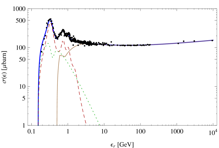
We show in LABEL:~1 the total photo-meson cross section as a function of , analogously to Mücke et al. (2000) (barn = cm2; data from Particle Data Group (2008))). The contributions of baryon resonances (red, dashed), the direct channel (green, dotted) and multi-pion production (brown) are shown separately.
In order to fully describe Eq. (9) for each interaction type, we need the kinematics, entering , the multiplicities , and the cross section .
3.2 Kinematics and secondary multiplicities
The kinematics for the resonances and direct production can be effectively described in the two-body picture. We follow the calculation of Berezinsky & Gazizov (1993) for the reaction with () in the SRF. The Lorentz factor between CMF and SRF is:
| (13) |
with the total CMF energy from Eq. (5). The energy of the pion in the SRF can then be written as:
| (14) |
with , and the pion energy, momentum and angle of emission in the CMF. Note that backward scattering of the pion means that . From Eq. (14) we can read off the fraction of energy of the initial going into the pion (which is equal to the inelasticity of for ). Since is a two body reaction, the energies of and pion are given by Particle Data Group (2008)
| (15) |
with given by Eq. (5). Using Eq. (15) in Eq. (14), we can calculate in Eq. (9) as
| (16) |
Indeed, is a function of if is a constant. As described in Rachen (1996), the average for the resonances (such as for isotropic emission in the CMF), whereas the direct production is backward peaked to a first approximation for sufficiently high energies . This approximation is only very crude. Therefore, we calculate the mean for direct production by averaging the probability distribution of the Mandelstam variable , as we discuss in App. A. Note that even for the resonances these scattering angle averages are only approximations; a more refined kinematics treatment, such as in SOPHIA, will lead to a smearing around these mean values. In addition, note that we also use Eq. (16) for the kaon production (with the rough estimate ), where the replacements and have to be made. Similarly, one has for the first and second pion for the interaction in Eq. (11) (Rachen, 1996)
| (17) | ||||
| (18) |
where , and for the interaction Eq. (12)
| (19) |
with . Note that in order to evaluate the -function in Eq. (9) (if one integrates over ), one also needs the derivative , which can easily be computed from the functions above.
| Initial is proton | Initial is neutron | Kinematics | ||||||||||
| IT | Eq. | |||||||||||
| Interactions | ||||||||||||
| - | - | (16) | ||||||||||
| - | - | (16) | ||||||||||
| T1 | - | - | - | - | - | - | (16) | |||||
| Interactions , | ||||||||||||
| Properties of first pion and nucleon | ||||||||||||
| (17) | ||||||||||||
| (17) | ||||||||||||
| T | - | - | (17) | |||||||||
| Properties of second pion | ||||||||||||
| (18) | ||||||||||||
| (18) | ||||||||||||
| T | (18) | |||||||||||
| Interactions , ( and summed over) | ||||||||||||
| (19) | ||||||||||||
| (19) | ||||||||||||
The average multiplicities for different types of resonances and direct production channels can be found in Table 1. The multiplicities of the pions add up to the number of pions produced (one or two), the multiplicities for the nucleons in the final state to one. They are needed in Eq. (6) and Eq. (B1) (cooling and escape timescale in App. B). In the last columns, the cosine of the approximate scattering angle in the center of mass frame is given, together with the equation for kinematics. The interaction types IT are labeled by the type of resonance ( or ) or for the direct production (-channel). Note that different resonances will contribute with a similar pattern, such as through the interaction types , , , , etc.. In addition note that the branching ratios into certain resonances and from a resonance into the described channels are absorbed in the cross sections. Therefore, the total yield is always one (or two) pions per interaction in Table 1.
For the multi-pion channel, we use two different approaches. A very simple treatment can be performed similar to Atoyan & Dermer (2003), with some elements of Mücke et al. (2000). Most of the energy lost by the proton (, or ) is split equally among three pions. The three types , , and are therefore approximately produced in equal numbers. Our multi-pion channel, parameterized by the multi-pion cross section in LABEL:~1, however, is actually a combination of different processes and residual cross sections. For instance, diffractive scattering is a small contribution. Therefore, in order to reproduce the pion multiplicities times cross sections in Figs. 9 and 10 of Mücke et al. (2000) more accurately, we choose (), (), and () for initial protons (neutrons). Close to the threshold, the decreasing phase space for pion production requires a modification of the threshold for () from initial protons (neutrons). This corresponds to a vanishing multiplicity below the threshold, i.e., we assume that below only two pions are produced. We assume for the fraction of the proton energy going into one pion produced in the multi-pion channel . In addition, we choose and for initial protons (or and for initial neutrons) in accordance with Fig. 11 of Mücke et al. (2000) for high energies. As alternative, we use a more accurate but computationally more expensive approach, which is directly based on the kinematics of the fragmentation code used by SOPHIA (cf., Sec. 4.4.2).
3.3 Cross sections
We parameterize the cross sections of photohadronic interactions following Mücke et al. (2000). We split the processes into three parts: resonant, direct, and multi-pion production. The different contributions are shown in LABEL:~1.
The low energy part of the total cross section is dominated by excitations and decays of baryon resonances and . The cross sections for these processes can be described by the Breit-Wigner formula
| (20) |
with given by Eq. (5). Here , , and being the spin, the nominal mass, and the width of the resonance, respectively. We consider the energy-dependent branching ratios and the resonances shown in the Appendix B of Mücke et al. (2000); the total branching ratios are also listed in Table 2. Note that the energy-dependent branching ratios respect the different energy thresholds for different channels (e.g., interaction types 1 to 4). For simplicity, we neglect the slight cross section differences between - and -interactions and use the values for protons, which implies that we do not take into account the N(1675) resonance.555For a more accurate treatment for neutrons, also include the N(1675) resonance, whereas N(1650) and N(1680) do not apply. In addition, in Eq. (25), replace and in Eq. (26), replace . In Table 2 we list all considered resonances and their contributions to the different interaction types. To account for the phase-space reduction near threshold the function is introduced and multiplied on Eq. (20):
| (21) |
with and taking the values shown in Table 2.
| Properties | Total | |||||||
|---|---|---|---|---|---|---|---|---|
| Resonance | [GeV] | [GeV] | [barn] | [GeV] | [GeV] | IT | IT | IT |
| 100% | - | - | ||||||
| 67% | 33% | - | ||||||
| 52% | 42% | 6% | ||||||
| 45% | - | - | ||||||
| 75% | 14% | - | ||||||
| 64% | 22% | 14% | ||||||
| 14% | 55% | 31% | ||||||
| 14% | 13% | 73% | ||||||
| 37% | 39% | 24% | ||||||
For the direct and the multi-pion cross section we adopt the formulae from SOPHIA. The direct part is given by
| (22) | ||||
| (23) |
with
| (24) |
where . The cross sections are given in barns, and the interaction types are taken from Table 1, i.e., T1 is the single pion direct production, and T2 is the two pion direct production. The multi-pion cross section can be parameterized by the sum of the following two formulas (cross sections in barns):
| (25) | ||||
| (26) |
We have compared our resonant and direct production multiplicities times cross sections and proton to neutron ratios with SOPHIA (cf., Figs. 9 to 11 in Mücke et al. (2000)), and they are in excellent agreement.
4 Simplified models
Here we discuss simplified models based on Sec. 3, where we demand the features given in the introduction. For the resonances, we propose two methods, one is supposed to be more accurate, the other one faster.
4.1 Factorized response function
First of all, it turns out to be useful to simplify the response function in Eq. (9). In our simplified approaches, we follow the following general idea: In Eq. (7) and Eq. (9), in principle, (at least) two integrals have to be evaluated. Let us now split up the interactions in interaction types such that and are approximately constants independent of , but dependent on the interaction type. The response function in Eq. (9) then factorizes in
| (27) |
The part describes at what energy the secondary particle is found, whereas the part describes the production rate of the specific species as a function of . If only the number of produced secondary particles is important, it is often useful to show the effective .
As the next steps, we evaluate Eq. (7) with Eq. (27) by integrating over and by re-writing the -integral as -integral:
| (28) |
This (single) integral is relatively simple and fast to compute if the simplified response function together with is given. Therefore, the original double integral simplifies in this single integral, summed over a number of appropriate interaction types. In the following, we therefore define , and for suitable interaction types.
4.2 Resonances
Here we describe two alternatives to include the resonances. Model A is more accurate but slower to evaluate, because it includes more interaction types, whereas model B is faster for computations, since there are only two interaction types defined for the resonances.
4.2.1 Simplified model A (Sim-A)
| Initial proton | Initial neutron | |||||||||
|---|---|---|---|---|---|---|---|---|---|---|
| IT | ||||||||||
| (1232) | 1.00 | 0.34 | 66.69 | 0.22 | - | - | ||||
| (1440) | 0.67 | 0.64 | 4.26 | 0.29 | - | - | ||||
| (1440) | 0.33 | 0.64 | 4.26 | 0.14 | ||||||
| (1440) | 0.33 | 0.64 | 4.26 | 0.19 | ||||||
| (1520) | 0.52 | 0.75 | 27.01 | 0.31 | - | - | ||||
| (1520) | 0.42 | 0.75 | 27.01 | 0.17 | ||||||
| (1520) | 0.42 | 0.75 | 27.01 | 0.18 | ||||||
| (1520) | 0.06 | 0.75 | 27.01 | 0.22 | ||||||
| (1535) | 0.45 | 0.77 | 6.59 | 0.32 | - | - | ||||
| (1650) | 0.75 | 1.03 | 3.19 | 0.35 | - | - | ||||
| (1650) | 0.14 | 1.03 | 3.19 | 0.23 | ||||||
| (1650) | 0.14 | 1.03 | 3.19 | 0.17 | ||||||
| (1680) | 0.64 | 1.04 | 15.72 | 0.35 | - | - | ||||
| (1680) | 0.22 | 1.04 | 15.72 | 0.24 | ||||||
| (1680) | 0.22 | 1.04 | 15.72 | 0.17 | ||||||
| (1680) | 0.14 | 1.04 | 15.72 | 0.23 | ||||||
| (1700) | 0.14 | 1.05 | 21.68 | 0.35 | - | - | ||||
| (1700) | 0.55 | 1.05 | 21.68 | 0.24 | ||||||
| (1700) | 0.55 | 1.05 | 21.68 | 0.16 | ||||||
| (1700) | 0.31 | 1.05 | 21.68 | 0.23 | ||||||
| (1905) | 0.14 | 1.45 | 3.03 | 0.38 | - | - | ||||
| (1905) | 0.13 | 1.45 | 3.03 | 0.29 | ||||||
| (1905) | 0.13 | 1.45 | 3.03 | 0.15 | ||||||
| (1905) | 0.73 | 1.45 | 3.03 | 0.23 | ||||||
| (1950) | 0.37 | 1.56 | 16.46 | 0.39 | - | - | ||||
| (1950) | 0.39 | 1.56 | 16.46 | 0.30 | ||||||
| (1950) | 0.39 | 1.56 | 16.46 | 0.15 | ||||||
| (1950) | 0.24 | 1.56 | 16.46 | 0.23 | ||||||
In this simplified resonance treatment we make use of the fact that the resonances have cross sections peaked in . In principle, these can be approximated from Eq. (20) and Eq. (21) by a -function
| (29) |
where and correspond to surface area (in barn-) and position (in GeV) of the resonance, and are process-dependent constants. Therefore, using Eq. (29), the -integral in Eq. (9) can be easily performed, and we obtain again the simplified Eq. (27) with
| (30) |
The relevant parameters for all interaction types can be read off from Table 3. Note that are the total (i.e., energy-independent) branching ratios from Table 2. In addition, note that in some cases, the resonance peak may be below threshold for some of the interaction types. However, for reasonably broad energy distributions to be folded with and the total branching ratios used, this should be a good approximation. The pion spectra are finally obtained from Eq. (28), summing over all interactions listed in Table 3.
4.2.2 Simplified model B (Sim-B)
In this model, we take into account the width of the resonances and approximate them by constant cross sections within certain energy ranges. Compared to approaches such as in Reynoso & Romero (2009), we distinguish between and production (i.e., do not add these fluxes) and include the effects from the higher resonances.
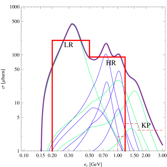
From LABEL:~1, one can read off that there are two classes of resonances: The first peak in LABEL:~1 is dominated by the -resonance (lower resonance – LR), whereas the higher resonances (HR) contribute at larger energies. In addition, the kinematics (cf., in Table 3) and the multiplicities (cf., Table 1) are very different. For example, protons and neutrons interactions via the -resonance happen through only one interaction type, and produce either only or only (and ). For the higher resonances, the pions are produced in all pion charges.
| IT | -range [GeV] | [barn] | Initial proton | Initial neutron | |||||||
| K | |||||||||||
| LR | 200 | 2/3 | 1/3 | - | 1/3 | 2/3 | - | 1/3 | 2/3 | 0.22 | |
| 0.22 | 0.22 | - | 2/3 | 0.22 | - | 0.22 | 1/3 | ||||
| HR | 90 | 0.47 | 0.77 | 0.34 | 0.43 | 0.47 | 0.34 | 0.77 | 0.57 | 0.39 | |
| 0.26 | 0.25 | 0.22 | 0.57 | 0.26 | 0.22 | 0.25 | 0.43 | ||||
For the resonances, we define two interaction types LR and HR, as shown in LABEL:~2 (boxes). The interaction type LR corresponds to , whereas the interaction type HR contains the higher resonances. The properties of these interaction types are summarized in Table 4.
The surface area covered by these cross sections, corresponding to the in simplified model A, is chosen for LR and HR such that the pion spectra match to these of the previous section for typical power law spectra (with spectral indices of about two). Of course, there can never be an exact match, because the contributions from the individual resonances depend on the spectral index. However, as we will demonstrate, this estimate is good enough for our purposes.
The averaged numbers for the multiplicities and inelasticities for the higher resonances interaction type are estimated from the interaction rate Eq. (4) by assuming that all resonances contribute simultaneously and weighting by the interaction type-dependent part (cf., Eq. (B3) using Eq. (30); cf., App. B). By the same procedure we obtain the average -values from Eq. (9). Note that the (for proton interactions) are, in average, reconstructed at lower energies, because these are mostly produced by interaction type 2, which has smaller -values (cf., Table 3). In addition, note that the total number of charged pions is, in fact, close to one per interaction here, and the total number of pions close to 1.5, since in interaction types 2 and 3 more than one pion is produced.
4.2.3 Comparison of resonance response functions
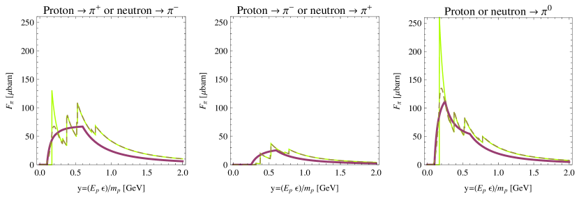
In LABEL:~3, we compare the response function between simplified model Sim-A (thin solid curves) and Sim-B (thick curves), summed over the resonances. This function is proportional to the number of produced pions of a certain species as a function of , whereas the -dependent part in Eq. (27) describes the energy at which the pions are found. Obviously, the function is much smoother for Sim-B than for Sim-A. Because of only a few contributing interaction types and the smoothness of the function, the evaluation will be much faster. Once the photon spectrum is folded in, the contributions of both response functions will be very similar.
Note that model Sim-B includes the part of the -resonance below the peak. This can be seen by comparing with the dashed curve, which represents model Sim-A but the interaction type replaced by the full Breit-Wigner-form.
4.3 Direct production
| Initial proton | Initial neutron | |||||||||
| IT | [GeV] | [GeV] | K | |||||||
| T | 0.13 | 0.13 | - | 1 | - | - | - | 1 | ||
| T | 0.05 | 0.05 | - | 1 | - | - | - | 1 | ||
| T | 0.001 | 0.001 | - | 1 | - | - | - | 1 | ||
| T | 0.08 | 0.28 | - | - | ||||||
| T | 0.02 | 0.22 | - | - | ||||||
| T | 0.001 | 0.201 | - | - | ||||||
| T | 0.2 | - | ||||||||
For direct production, we also follow the approach in Sec. 4.1. However, this interaction type is tricky, since the kinematics function is strongly dependent on the interaction energy (see App. A for details). This implies that the -distribution in Eq. (6) is not a good approximation and needs to be replaced by a broader distribution function. In addition, the distribution of scattering angles will lead to smearing effects. In this case, it turns out to be a good approximation to split the direct production in different interaction types with different characteristic values of as a function of , which simulates such a broad distribution after the integration of the input spectra. We define three interaction types , , and for direct one pion production and four for two pion production, namely , , and for the first pion, and for the second pion. The interaction types are shown in Table 5, and the names correspond to Table 1, split into low (L), medium (M), and high (H) energy parts in , respectively, limited by and . After this splitting, the additional effect of the scattering angle smearing turns out to be small, as we will demonstrate later. We obtain the function for these interaction types from Eq. (27) as
| (39) |
with re-parameterized using :
| (46) | |||||
| (49) |
Note that , , the multiplicities and can be read off from Table 5 for the different interaction types. The integral values are the same for interaction types , , (Eq. (46)), and for interaction types , , , and (Eq. (49)). In Eq. (28), all the interaction types in Table 5 have to be summed over.
4.4 Multi-pion production
Here we show two different approaches to the multi-pion channel. The first, simplified approach will later be shown as model Sim-C, the second, more refined approach will be used in all other models.
4.4.1 Simplified kinematics
We start with the simplest example for multi-pion production, for which we follow Sec. 3.2. We assume , i.e., the response function factorizes as . We obtain from Eq. (27) and Eq. (28)
| (50) |
with
| (51) |
As described in Sec. 3, we assume that (), (), and () for initial protons (neutrons). The function can be obtained using the sum of Eq. (25) and Eq. (26). We numerically integrate it and re-parameterize it with by
| (52) |
for , and (initial proton) or (initial neutron), and
| (53) |
for (initial proton) or (initial neutron). Note that the different function for comes from the different threshold below which we have set the cross section to zero, as discussed in Sec. 3.2. For , this function still increases as extrapolation of LABEL:~1 (the cross section is not measured in that energy range).
4.4.2 Kinematics simulated from SOPHIA
| Initial proton | Initial neutron | ||||||||||
|---|---|---|---|---|---|---|---|---|---|---|---|
| IT | [GeV] | [GeV] | K | ||||||||
| M | 0.5 | 0.9 | 60 | 0.1 | 0.27 | 0.32 | 0.34 | 0.04 | 0.32 | 0.04 | 0.34 |
| M | 0.5 | 0.9 | 60 | 0.4 | – | 0.17 | 0.29 | 0.05 | 0.17 | 0.05 | 0.29 |
| M | 0.9 | 1.5 | 85 | 0.15 | 0.34 | 0.42 | 0.31 | 0.07 | 0.42 | 0.07 | 0.31 |
| M | 0.9 | 1.5 | 85 | 0.35 | – | 0.19 | 0.35 | 0.08 | 0.19 | 0.08 | 0.35 |
| M | 1.5 | 5.0 | 120 | 0.15 | 0.39 | 0.59 | 0.57 | 0.30 | 0.59 | 0.30 | 0.57 |
| M | 1.5 | 5.0 | 120 | 0.35 | – | 0.16 | 0.21 | 0.13 | 0.16 | 0.13 | 0.21 |
| M | 5.0 | 50 | 120 | 0.07 | 0.49 | 1.38 | 1.37 | 1.11 | 1.38 | 1.11 | 1.37 |
| M | 5.0 | 50 | 120 | 0.35 | – | 0.16 | 0.25 | 0.23 | 0.16 | 0.23 | 0.25 |
| M | 50 | 500 | 120 | 0.02 | 0.45 | 3.01 | 2.86 | 2.64 | 3.01 | 2.64 | 2.86 |
| M | 50 | 500 | 120 | 0.5 | – | 0.20 | 0.21 | 0.14 | 0.20 | 0.14 | 0.21 |
| M | 500 | 5000 | 120 | 0.007 | 0.44 | 5.13 | 4.68 | 4.57 | 5.13 | 4.57 | 4.68 |
| M | 500 | 5000 | 120 | 0.5 | – | 0.27 | 0.29 | 0.12 | 0.27 | 0.12 | 0.29 |
| M | 5000 | 120 | 0.002 | 0.44 | 7.59 | 6.80 | 6.65 | 7.59 | 6.65 | 6.80 | |
| M | 5000 | 120 | 0.6 | – | 0.26 | 0.27 | 0.13 | 0.26 | 0.13 | 0.27 | |
Similar to the direct production, the -distribution in Eq. (6) is not a good approximation and needs to be replaced by a broader distribution function. We again solve this by splitting the multi-pion production in different interaction types with different characteristic values of , which simulates such a broad distribution after the integration of the input spectra. Compared to the direct production, the cross section can be parameterized relatively easily by step functions. However, the pion multiplicities in fact increase with energy. This means that the higher the interaction energy, the more pions are produced, which (in average) are found at lower energies. In addition, the final energy distribution functions are broad.
We solve this strongly scale-dependent behavior by dividing the -range in seven interaction types Mi, each with a particular average cross section and average pion multiplicities, which we directly take from SOPHIA. In addition, we split the pions in each of these samples in a lower energy (L) and higher energy (H) part, which are reconstructed at different values of to simulate the broadth of the distributions within the same . Typically, the -sample corresponds to the peak of the distribution (at least for high energies), whereas the H-sample simulates the tail of the distribution. The splitting of the multiplicities can be performed automatically once a splitting point is defined. We choose the -values of the interaction types to simulate the peaks of the distribution and to reproduce the total energy going into pions in SOPHIA. This treatment is, of course, not extremely accurate, but it allows to use the fast approach in Eq. (27) while obtaining accuracy at high energies.
The function can be easily calculated from Eq. (27) since the cross section is assumed to be constant within each IT:
| (54) |
The interaction types are listed in Table 6, where the parameters for this equation can be found, as well as the and values and multiplicities for the individual interaction types.
4.5 Kaon production
Here we include production into our simplified model. If needed, other (sub-leading) channels can be added to our framework as well (such as production if the neutrino-antineutrino ratio in the higher energy regime is studied). This example should also serve as illustration how to add processes to our model. Note that this implementation, however, is more primitive than the pion production above.
The production of in photohadronic interactions cannot be assigned to a single resonance, but comes from a number of resonances mainly decaying into and or (with relatively similar masses, which means that we can neglect the mass difference). In addition, at high interaction energies, multi-fragmentation, similar to multi-pion production, contributes significantly. The production cross section up to has been measured (Saphir Collaboration, 1998). For higher energies, where no data are available, one may use extrapolations from models (Lee et al., 2001; Asano & Nagataki, 2006). Approximating the data in Lee et al. (2001) and extrapolating according to Lee et al. (2001), we define an interaction type “KP” and model the total production cross section as (cf., dashed curve in LABEL:~2)
| (59) |
Accordingly, we obtain the response function from Eq. (27) with :
| (64) |
From Sec. 3.2, we have (computed for at the peak). The effects on primary cooling and secondary re-injection in App. B are negligible. Note that the absolute normalization of the kaons at high energies crucially depends on the extrapolation of the cross sections to high energies. Our kaon production is about a factor of two smaller at higher energies than in Lipari et al. (2007), since we assume the cross section to be constant at high energies.
4.6 Comparison of individual contributions
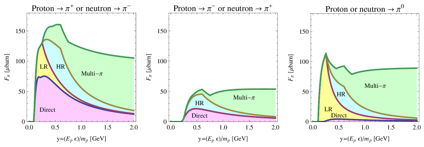
In LABEL:~4, we show the individual contributions to for pion production as a function of , which is proportional to the maximal available center-of-mass energy. This quantity describes the total number of pions of a particular species produced as a function of , including multiplicity and cross section. However, it does not include the energy where the pions are found. For initial protons, are most abundantly produced because of the direct production contribution, followed by and then . For production close to the threshold, the direct production and resonances are most important, whereas for production, the direct production hardly has any impact, and the resonances dominate. For production, at the threshold all processes contribute almost equally, only the lower resonance does not take part. For larger , in all cases multi-pion production dominates.
As far as the relative contribution is concerned, thanks to the direct production, the are always produced most abundantly. As one can read off from LABEL:~4, this statement is independent of the photon or proton spectra used, because the response function for is always larger than the one for , in a large part of the energy range even about 50% larger. This means that for arbitrary proton and photon spectra, thanks to the direct production, the : ratio lies between about 1:1 and 3:2, whereas the -approximation in Eq. (1) predicts 1:2. In fact, one can show that the minimum of the charged to neutral pion ratio with respect to is
| (65) |
for arbitrary input spectra; see Mücke et al. (2000) for a specific photon field.666As mentioned above, does not include the reconstructed energy of the pions. Since, however, the pions of the different species are found in similar energy ranges, this statement also roughly applies to the energy deposited into the different species. From this equation, any neutrino flux computed with the -approximation and normalized to the observed photon spectrum, if mainly coming from decays, is underestimated by a factor of at least , i.e., the neutrino flux should be about a factor of 2.4 larger. Even the often used approximation that 50% of all photohadronic interactions result in charged pions underestimates the neutrino flux by at least 20%. These numbers are to be interpreted as lower limits for the neutrino flux underestimation, the exact values depend on the input spectra and may be even higher.
Of course, the overall impact of the individual contributions depends on the proton and photon spectra the response function is to be folded with. In order to check the impact of the individual contributions on typical AGN, GRB or high temperature black body (BB) spectra, we define three benchmark spectra in App. C. Note that all of the spectra shown in this work are given in the SRF.
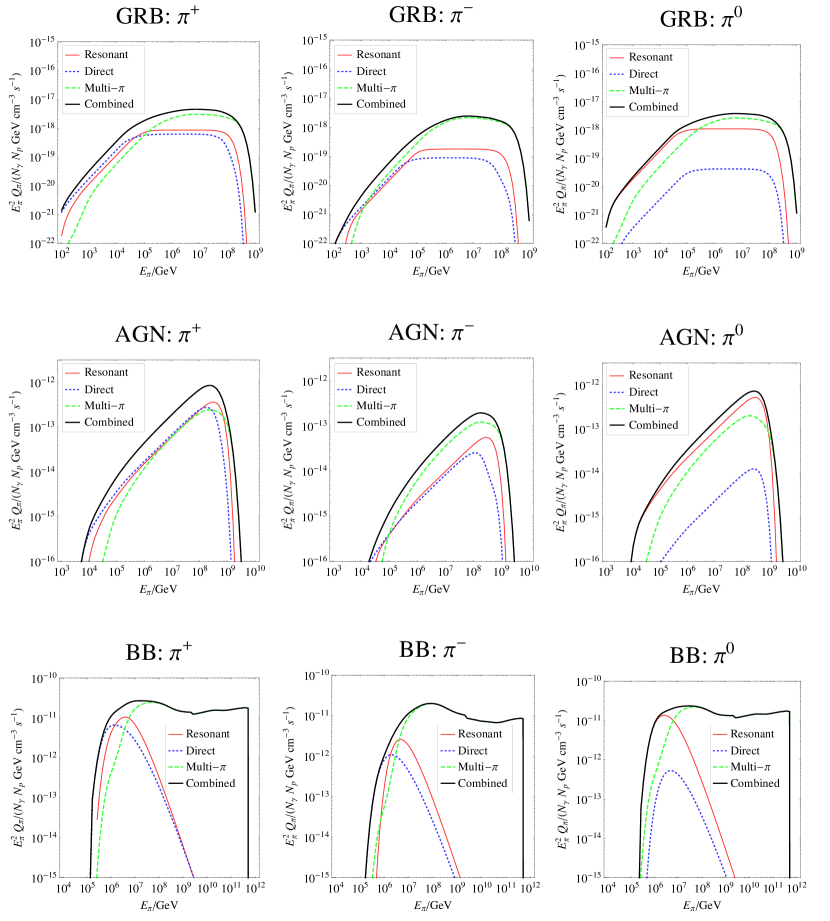
In LABEL:~5, we show the , , and spectra for these benchmarks. The upper panels are for the GRB benchmark, the middle ones for the AGN benchmark and the lower ones for the BB benchmark. For the GRB benchmark, direct production dominates at low energies for the production, whereas the production at low energies is determined by the resonances. The production is dominated at all energies by the multi-pion production, such as the other spectra at high energies. Therefore, all different processes are important, but they contribute entirely different to the different pion polarities. One can also read off from this figure, that the characteristic shape of the GRB pion or neutrino spectra often shown in the literature (resonance curves), which is flat in the middle energy range, is tilted upwards due to multi-pion production. For the AGN benchmark (middle panels), the production is governed by the resonances in the whole energy range, the production by the multi-pion production, and the production by similar contributions of all processes including the direct production. In this case, the -resonance approximation is more accurate in terms of the shapes of the spectra. However, other processes quantitatively contribute as well. For the BB benchmark (lower panels), the production is dominated by the multi-pion production for most of the energies. Only in the low energy region, the charged pion production is governed by the direct and the resonant processes, and the production by the resonances. In this case, ignoring the high energy processes would lead to clearly misleading results.
As far as the comparison among the different polarities is concerned, see LABEL:~6. For all spectra, the are always most abundantly produced, as predicted above, followed by and then . For the GRB benchmark at high energies, where the multi-pion production dominates, the spectra are closest to each other. At low energies, there are significantly less produced than the other two polarities. However, note that, thanks to the multi-pion production, the are only suppressed by a factor of a few. The kaons, on the other hand, contribute about one to two orders less to the total meson fluxes. Nevertheless, there can be interesting effects in the high energy regime if cooling effects are present. For the AGN benchmark, because of the lower maximal proton energy times photon energy, even for large energies the are strongly suppressed. Otherwise, the result is qualitatively similar. For the BB spectrum we can nicely see the effect of lower multiplicities of compared to and for high interaction energies (see Table 6) in the spectrum at energies higher than . Otherwise, we have similar results as for the GRB benchmark.
5 Comparison with SOPHIA
Here we compare the results of our simplified models with each other and with SOPHIA. First, we focus on the primaries produced in the photohadronic interactions, mostly the pions. Then we compute and compare the neutrino spectra. In all cases, we use initial protons for the photohadronic interactions.
5.1 Pion spectra
| Abbrev. | Description | Complexity | Sec./Refs. |
|---|---|---|---|
| SOPHIA | SOPHIA software with full kinematics | Monte Carlo method, | Mücke et al. (2000) |
| BW | Resonances with full Breit-Wigner description; direct production with full response function; simple kinematics | Double integration, 45 IT, | Sec. 3 incl. multi-pion from Sec. 4.4.2 |
| Sim-A | Simplified model with factorized response function and resonance treatment A (-function approximation) | Single integration, 49 IT, | Sec. 4 with Sec. 4.2.1 and Sec. 4.4.2 |
| Sim-B | Simplified model with factorized response function and resonance treatment B (step function approximation) | Single integration, 23 IT, | Sec. 4 with Sec. 4.2.2 and Sec. 4.4.2 |
| Sim-C | Simplified model with factorized response function and resonance treatment B; simplified multi-pion production | Single integration, 10 IT, | Sec. 4 with Sec. 4.2.2 and Sec. 4.4.1 |
The models considered in this subsection are listed in Table 7, where the (computational) complexity decreases from the top to the bottom. “SOPHIA” represents the output of the SOPHIA software, computed for our benchmark spectra from App. C. The computation with SOPHIA is described in App. D. The model “BW” corresponds to the basic physics of SOPHIA as described in Sec. 3, including double integration for the direct production and multi-pion production from Sec. 4.4.2. In this case, we use Eqs. (7) and (9) for the secondary production using the two dimensional response function including all resonances with full Breit-Wigner forms and the direct production as described in App. A. Compared to SOPHIA, the kinematics is considerably simplified. The multi-pion production is taken from Sec. 4.4.2 close to SOPHIA. “Sim-A” and “Sim-B” are the simplified models from Sec. 4, using the factorized response function introduced in Sec. 4.1. Whereas Sim-A treats all interaction types with the resonances explicitely, Sim-B defines an interaction type for the -resonance, and one for the higher resonances. Therefore, Sim-B uses considerably less interaction types. Note that we have obtained Sim-A and Sim-B by condensing the information from BW stepwise. Both models use the multi-pion production from Sec. 4.4.2, whereas Sim-C is a simplified version of Sim-B including the multi-pion production in Sec. 4.4.1.
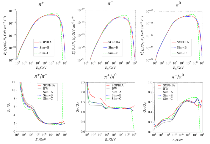
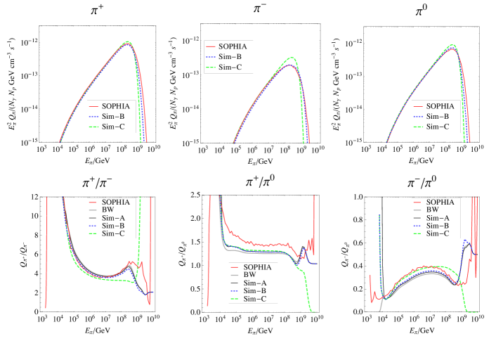
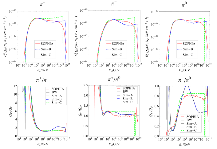
We compare the pion spectra produced by these different models in LABEL:~7 (GRB benchmark), LABEL:~8 (AGN benchmark) and LABEL:~9 (Black body (BB) benchmark). In these figures, the upper rows show the pion spectra for , , and explicitly, whereas the lower rows show the pion ratios , , and . Since the pion spectra for model BW, Sim-A and Sim-B are so close to each other that they can not be distinguished, we plot only the results of SOPHIA, model Sim-B and model Sim-C in the upper rows of Figs. 7 to 9. Whereas the charged pions lead to neutrino production, the neutral pions lead to photons. Therefore, the ratio determines, to leading order, the ratio between neutrinos and photons, which also often enters the computation of neutrino flux limits. On the other hand, the ratio affects the (electron) neutrino-antineutrino ratio. The ratio is shown for completeness. Note that the normalization of the different spectra is not chosen arbitrarily, but consistently to be able to compare the spectra directly; cf., App. D.
As the most important fact, as it can be read off from the upper rows of the three figures, all the spectra of our simplified models (apart from Sim-C, maybe) match the output from SOPHIA very well, both normalization and spectral shape. At high energies, however, where we imposed a sharp spectral cutoff, the spectra from SOPHIA are smeared out because of the more refined kinematics treatment, which can best be seen in LABEL:~9 for the BB benchmark where we have a sharp spectral cutoff in the proton spectrum. This difference is unavoidable, and the price to pay for an efficient simplified model. Nevertheless, note that in more realistic spectra, or spectra averaged over different sources, such sharp features in the spectra may not be present. Although it seems that there are hardly any differences between SOPHIA and our models at lower energies, one can read off from the pion ratio plots in the lower rows (on a linear vertical scale) that there are small deviations. Whereas the differences at very low and high energies, where the spectra rapidly break off, are not very surprising, there are some differences coming from the different kinematics treatment. For example, SOPHIA actually produces even about 20% more than in the lower energy range for the GRB benchmark and the middle energy range for the AGN benchmark (cf., middle lower panels). We have checked that this difference neither comes from the resonance or direct production treatment, nor from the relative contribution of both processes. Instead, for some processes, our kinematics is a bit over-simplified, since for these a considerable amount of pions is (in SOPHIA) reconstructed at lower energies. Another example for an obvious difference is the high energy / and / difference in the lower panel of LABEL:~9 for the BB benchmark, the most challenging one for the treatment of multi-pion production. The discrepancy is a result of the simplified kinematics treatment of taking the same -values for , and . This mainly effects the spectra because they have, in comparison to and , slightly different kinematics in SOPHIA. In the upper panel in LABEL:~9 a double hump structure can be seen which follows from the kinematics treatment of multi-pion production that one part of the pions is reconstructed at lower energies (small ) and the other at higher energies (large ). If one averages over larger energy scales (such as in diffuse fluxes), such kinematics effects average out.
As far as the comparison among our simplified models is concerned, the differences are small compared to the effects of kinematics discussed above. In fact, model “BW”, which was originally designed as the most accurate reproduction of SOPHIA, produces the results farthest off from SOPHIA, especially for the lower half of the energy range. The reason may be that the errors introduced by the approximations in Sim-A and Sim-B partly compensate the errors from the simplified multi-pion production and direct channels. The model Sim-A was obtained from BW by assuming that all resonances are strongly peaked, whereas Sim-B was derived from this assumption by collecting the properties of the higher resonances into one interaction type. In the comparison of model Sim-B to Sim-C the differences between the kinematics for multi-pion production from Sec. 4.4.2 and the simplified one from Sec. 4.4.1 can nicely be seen. For the GRB (see LABEL:~7) and the AGN benchmark (see LABEL:~8) this mainly effects the high energy region whereas in the BB case (see LABEL:~9) most of the energy range is affected. Since the computation time for Sim-B, for which the results do not differ significantly from model Sim-A, is only about a factor of 2-3 longer and the high energy treatment is way more accurate than for Sim-C (especially close to the peaks), we focus in the following on model Sim-B. As one can see in Figs. 7 to 9, Sim-B is most accurate for power laws which are our main interest. Compared to SOPHIA, we gain a factor of about 1000 (if implemented in C, depending on the integration method) in computation time for 100000 trials per proton bin in SOPHIA (as we use for the GRB benchmark). The Sim-B spectra do not have any small wiggles, because the computation is exact. However, note that the complexity of Sim-B increases with the number of interaction types, whereas the complexity of SOPHIA increases with the number of trials (and required smoothness of the functions).
5.2 Neutrino spectra
In this section, we first review the production of neutrinos from pion and subsequent muon decays, as well as kaon decays. For the sake of completeness, we include the neutrinos from neutron decays, where the neutrons are produced by the photohadronic interactions. Then we compare our results to SOPHIA. We focus on model Sim B from the previous section only.
The neutrinos are mostly produced in the following two decay chains:
| (66) | |||||
| (67) | |||||
For the energy spectrum from weak decays, we follow Lipari et al. (2007) (Sec. IV). In this case, the decays are described by Eq. (2). The functions simplify, in a frame where the parent is ultra-relativistic, to . The functions include the measured branching ratios in the possible final states and are given in Lipari et al. (2007) (Sec. IV). Note that and are initially produced in different ratios and produce muons with different helicities, described by the scaling functions with :
| (68) | |||||
| (69) |
The muons decay further in a helicity-dependent way:
| (70) | |||||
| (71) |
with for right-handed and for left-handed muons. It is therefore mandatory to distinguish four muon states , , , and as final states in order to account for the impact of muon polarization. The decay rates in Eq. (2) (there is only one interaction type, which is decay) are just the inverse lifetimes , where is the rest frame lifetime.
For kaons, the leading decay mode into muon and neutrino is treated in the same way as in Lipari et al. (2007) for the pion decays, i.e., with . The branching ratio for this channel is about 63.5%. The second-most-important decay mode is (20.7%). The other decay modes account for 16%, no more than about 5% each. Since interesting effects can only be expected in the energy range with the most energetic neutrinos, we only use the direct decays from the leading mode.
For protons accelerated in the jet, neutrons are produced by photohadronic interactions as described in App. B. Assuming that the neutrons escape from the acceleration region before they interact again, an additional neutrino flux from neutron decays is obtained. In this section, we show this neutrino flux separately. The beta decay describes the decay of the neutron into a proton, an electron and an electron anti-neutrino. In the ultra-relativistic case, the mean fraction of the neutron energy going into the neutrino is , see (Lipari et al., 2007). The neutrino spectrum is therefore obtained from the following equation:
| (72) |
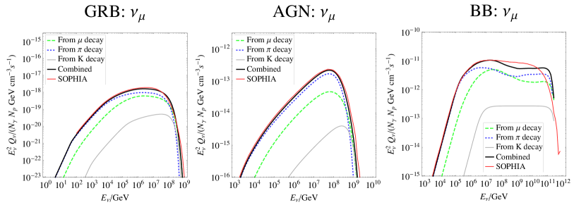
We show the neutrino spectra obtained from Sim-B and SOPHIA in LABEL:~10, where we also show the different contributions from different decay modes separately. Obviously, the SOPHIA and our combined spectra match very well, apart from the already discussed difference in the kinematics leading to some averaging in SOPHIA for large energies. Since the production of dominates for initial protons, in LABEL:~10 are most abundantly produced from pion decay; cf., Eq. (66). However, the from muon decays, coming from the decay chain – cf., Eq. (67) – are found at slightly higher energies and dominate for every high energies in the spectrum. For , the situation is exactly the opposite, but the final spectra look very similar. For very high energies, the SOPHIA spectrum is slightly higher than what one would expect, because other decay modes (such as from neutral kaons) contribute, which we have not considered. Without synchrotron cooling, the contribution from kaon decays is, however, small.
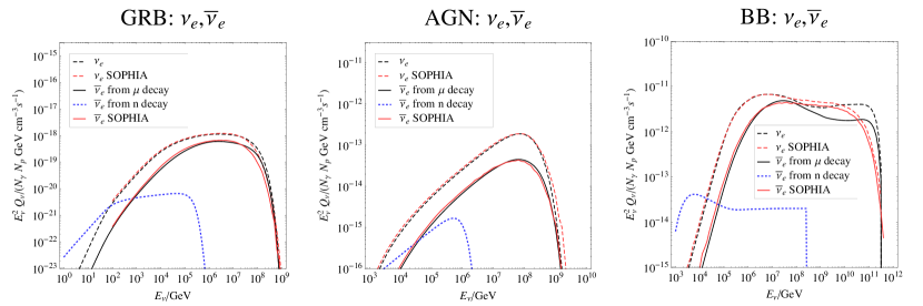
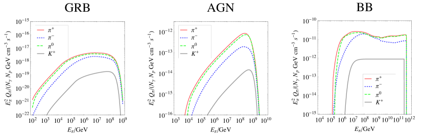
In LABEL:~11, we show the (dashed) and (solid) fluxes for our benchmarks. Obviously, the , coming from the decay chain in Eq. (66), dominate over the . However, if the neutrons produced by the photohadronic interactions escape from the source and then decay, they will lead to an additional neutrino flux shown by the thin gray curves (not included in the total curves). Especially at very low energies, the flux then dominates.
5.3 Flavor and neutrino-antineutrino ratios of the neutrinos
In this section, we discuss the electron to muon neutrino flavor ratio (the ratio between the electron and muon neutrino fluxes) and the neutrino-antineutrino ratios at the source. The flavor composition at the source is primarily characterized by the flux ratio , since almost no (or ) are expected to be produced at the source. Because neutrino telescopes can, in muon tracks or showers, not distinguish neutrinos from antineutrinos, this ratio is representative for the detection as well. From Eqs. (66) and (67), we can read off that this flavor ratio should be about without kinematical effects, which we call the “standard assumption”. At the Earth, the three neutrino flavors then almost equally mix (in the ratio 1:1:1) through neutrino flavor mixing (Learned & Pakvasa, 1995).
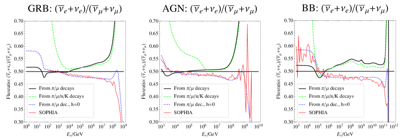
We show in LABEL:~12 the flavor ratio at the source for the GRB (left panel), AGN (middle panel) and BB (right panel) benchmark. The standard assumption 1/2 is marked by the horizontal lines. Our curves from Sim-B (thick solid, neutrinos from pion and muon decays only) bend upward from this standard assumption, whereas the SOPHIA curves bend downward for large energies. This difference can be explained by a different implementation of the weak decays: if we do not take into account the spin state of the final muon (dotted curves ), we can reproduce the SOPHIA results almost exactly with Sim-B. In fact, the effect of the helicity is larger than the details of the interaction model. The dashed curves include the effect of neutron decays (low energies) and kaon decays (high energies) into Sim-B. Especially for low energies, where are abundantly produced by neutron decays, the curves deviate from the thick ones. This effect is strongest for the AGN benchmark, for which the standard assumption 1/2 only approximately holds in a relatively narrow energy window. Note that the dashed curve in the left panel and all the other results for the GRB benchmark exactly match Lipari et al. (2007), where the weak decays are discussed in detail.
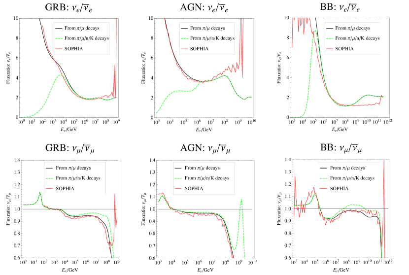
If the Glashow resonance process at around can be observed in a neutrino telescope, the neutrino-antineutrino ratios at the source may be relevant as well (all flavors at the source contribute to the flux at the Earth through flavor mixing) (Learned & Pakvasa, 1995; Anchordoqui et al., 2005; Bhattacharjee & Gupta, 2005). The neutrino-antineutrino ratio may be relevant to distinguish interactions at the source, for which mostly are produced, from interactions at the source, for which and are produced in almost equal ratios. Therefore, we show in LABEL:~13 the neutrino-antineutrino ratios at the source for electron neutrinos (left panels) and muon neutrinos (right panels). The electron neutrino-antineutrino ratios in the left panels depend on the ratio of and produced, see Eqs. (66) and (67). Our result matches SOPHIA very well, especially in the important energy range from the peak of the spectrum two decades down, apart from the discrepancy for high energies for the BB benchmark (upper right panel) which we discussed already as it is coming from the ratio. The deviation between SOPHIA and Sim-B can be up to 30%. After flavor mixing, the correction to the electron neutrino-antineutrino ratio at the Earth is at the level of 10%, much smaller than the effect on the flavor mix expected from interactions. The muon neutrino-antineutrino ratios in the right panels do not depend on the ratio of and produced, as in every pion decay the same number of muon neutrinos and antineutrinos is produced; see Eqs. (66) and (67). In this case, our results match SOPHIA and the standard prediction very well, and the effects of neutron and kaon decays are small in the absence of cooling.
6 Summary and conclusions
We have discussed simplified models for photo-meson production in cosmic accelerators. The main purpose of this simplification has been the definition of a photohadronic interaction model useful for efficient modern time-dependent AGN and GRB simulations, and for large-scale parameter studies, such as of neutrino flavor ratios. The major requirements have been listed in the introduction. For example, the secondaries (pions, kaons) are not to be integrated out, since their synchrotron cooling affects the neutrino flavor ratios.
We have first re-phrased the problem in terms of a two-dimensional “response function” to be folded with arbitrary photon and proton input spectra in order to compute the secondary fluxes. The key idea for our simplified models has been the factorization of this two-dimensional response function, which has allowed to eliminate one of the integrations. In order to include kinematics as good as possible, we have then defined a discrete number of different interaction types with different characteristics based on the underlying physics of SOPHIA. The kinematics of more complicated interactions, such as direct production or multi-pion production, has been simulated by the introduction of multiple interaction types for each production channel. In a step-by-step fashion we have simplified then the resonance treatment in order to arrive at our simplified model Sim-B. It allows for the computation of pion spectra with only one integral, summed over about ten interaction types, and can be easily adopted from our description. The extendibility of this approach has been demonstrated by showing how fluxes can be added, once a suitable parameterization is found.
Similarly, the response function can be easily changed if new data are provided, new processes can be included, or systematics on the particle physics can be added. Of course, some effort has to be spent to find a suitable parameterization for each process.
We have demonstrated that our results match the output of SOPHIA sufficiently well. However, there are some differences due to the more refined kinematics treatment of SOPHIA, which effectively corresponds to one additional integration. For example, for very narrow spectral features, such as rapid cutoffs, the spectra are naturally more smeared out by SOPHIA. This is especially the case for high energetic interactions where multi-pion production is dominant, as can be seen in the BB (black body) benchmark. However, our approach is much simpler in the sense that the interaction rate and the folding with the proton spectra is automatically taken into account (cf., App. D). In addition, we have included the spin state of the final muon in the pion decays, as described in Lipari et al. (2007), not included in SOPHIA, which leads to differences in the neutrino flavor ratios: in fact, the electron to muon neutrino flavor ratio at the source is typically larger than 0.5, instead of smaller, as predicted without taking into account the spin state. In particular, we obtain for the GRB benchmark, for the AGN benchmark, and up to for the BB benchmark close to the spectral peaks. This means that especially the AGN benchmark behaves as pion beam in spite of the helicity dependence of the muon decays, whereas the BB benchmark shows the strongest deviation.
Since our approach has allowed us to discuss the leading interaction types separately, we have also shown the differences to the -resonance approximation (see also Mücke et al. (2000, 1999)). For example, we have shown how multi-pion production modifies the characteristic shape of the GRB neutrino spectrum expected from the resonance approximation (which is flat in times the flux in the intermediate energy range). In fact, all of the the resonances combined do not dominate in any significant part of the charged pion spectrum for our GRB, AGN and BB benchmarks. In addition, the -resonance approximation has rendered insufficient for the computation of the (electron) neutrino-antineutrino ratios at the source, because, by definition, no are produced. We have also demonstrated from our general response function in model Sim-B, that for any input proton or photon spectrum the ratio at the source is significantly larger than one, as opposed to 1/2 from the -resonance approximation. This implies that any neutrino flux based on the -resonance approximation and normalized to photon flux observations using the charged to neutral pion ratio is underestimated by at least a factor of , where this factor is independent of the input spectra.
We conclude that our simplified model Sim-B allows for an efficient computation of pion and neutrino fluxes, including the necessary features for neutrino flux ratio discussion and the necessary efficiency for time-dependent simulations. It is sufficient for many purposes especially for power law photon fields, but, of course, it cannot replace a full Monte Carlo simulation including full kinematics if high precision fits of existing data are required. In particular, it may turn out to be useful for time-dependent simulations and extensive parameter space studies using power law spectra, including spectral breaks. However, in other cases, such as if the high energy interactions with photon spectra with sharp peaks are very important, or there are anisotropic photon distributions, the Monte Carlo method may be the better choice.
Acknowledgments
We would like to thank M. Maltoni, K. Mannheim, D. Meloni, and A. Reimer for useful discussions. SH acknowledges support from the Studienstiftung des deutschen Volkes (German National Academic Foundation). FS acknowledges support from Deutsche Forschungsgemeinschaft through grant SP 1124/1. WW would like to acknowledge support from the Emmy Noether program of Deutsche Forschungsgemeinschaft, contract WI 2639/2-1. This work has also been supported by the Research Training Group GRK1147 “Theoretical astrophysics and particle physics” of Deutsche Forschungsgemeinschaft.
Appendix A Kinematics treatment of direct production
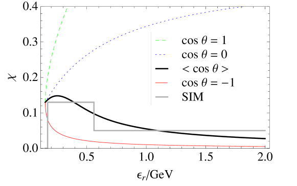
Here we follow the approach of Rachen (1996). As mentioned in Sec. 3.2, the direct production process is strongly backward peaked with respect to the produced pion. One possible approximation for the determination of is to assume that the average scattering angle is . The energy fraction going into the pion as a function of is shown in LABEL:~14 as the curve (cf., Eq. (16)). For comparison, the curves and are shown as well. For a more accurate representation of kinematics, we take the probability distribution of the Mandelstam variable , as given in Mücke et al. (2000), into account. For small , it is given by:
| (A1) |
with . For example, for the interaction type , the Mandelstam variable is given by
| (A2) |
Combining Eqs. (A1) and (A2), we obtain the average scattering angle as a function of the center-of-mass energy. Inserting the result into Eq. (16), we obtain the average energy fraction going into the pion for direct one pion production. It is shown in LABEL:~14 as curve “” as a function of . Analogously we compute the mean for direct two pion production by combining Eq. (A1) with the variable for the considered process.
In the simplified model for direct production (cf., Sec. 4.3) we use the factorized response function (see Eq. (27)) as for the simplified models of the other processes. Therefore we have to choose an energy independent, constant . Since the range of -values for direct production is wide, we divide the -range into three sections (for each of the interaction types and ), such that it reproduces the results of the non-simplified model for typical power law spectra for photons and protons in astrophysical sources, such as GRBs and AGNs. This approach corresponds to the thick gray curve “SIM” in LABEL:~14, where only the lower two interaction types are visible in the plotted energy range. Obviously, it is a good step function approximation to the curve “”. The different sections of this step function correspond to our interaction types “L”, “M”, and “H”.
Appendix B Cooling and escape of primaries, re-injection
A related issue to the secondary particle production is the cooling or escape of the primaries due to the interaction process. We do not focus on the cooling or escape timescales in this study, but, for the sake of completeness, we demonstrate how they can be computed from the quantities presented for our simplified models in Sec. 4. If the primaries lose energy in an interaction, such as protons or neutrons in pion photoproduction , this process can be interpreted as cooling, whereas if the primaries disappear, such as protons in , it can be interpreted as escape. In the latter case, neutrons are re-injected into the system, which we will discuss below. The cooling rate or escape rate for the species (proton or neutron) due to the photohadronic interactions is, for constant , given by
| (B1) |
in terms of the quantities in Eq. (2). Here is the loss of energy per interaction; therefore, is often called “inelasticity”. Note that if it is a function of the kinematical variables, such as the center of mass energy, it has to be folded into the calculation of the interaction rate in . However, in Sec. 4, we have constructed the interaction types such that is a constant. For photo-pion production, the inelasticity can be related to the in Eq. (6) by
| (B2) |
i.e., the energy loss of the nucleon equals the energy deposited in all interaction products (other than the initial nucleon). Note that the classification as cooling or escape also depends on if protons and neutrons are distinguished in the final state. In this section, we distinguish protons and neutrons. In addition, note that in astrophysical objects there may be other sources of cooling and escape to be taken into account, such as synchrotron cooling or escape from the production region.
The quantity needed for the computation of Eq. (B1) is the interaction rate in Eq. (4). Comparing Eq. (4) with Eq. (27), we find for our simplified models that the interaction rate for interaction type IT of the initial nucleon is
| (B3) |
i.e., conveniently parameterized in terms of our simplified response function. Then the cooling and escape rates in Eq. (B1) can be written in terms of the initial or different nucleon multiplicity ():
| (B4) |
The nucleon multiplicities are for the resonances in model A given in Table 1 for the interaction types in Table 3, for the resonances in model B in Table 4, for multi-pion production and , and for direct production in Table 1 for the interaction types in Table 5. The inelasticities can in resonance model A be obtained from the in Table 3 according to Eq. (B2), i.e., , where the number of pions produced for ITs 1, 2a, and 2b, and for IT 3 (for IT 2, the pions in 2a and 2b are summed over). For resonance model B, they are given in Table 4, for multi-pion production , and for direct production they are listed in Table 5 (here IT is not counted separately).
The re-injection rate for initial nucleons can be obtained analogously to Eq. (27) and Eq. (28) from
| (B5) |
as
| (B6) |
Note that double counting of the same interaction has to be avoided. In particular, interaction type 2 must not be counted twice.777Although there are two pions produced, there is only one secondary nucleon. For the inelasticity, however, the energy losses into all pions have to be taken into account. For the interaction rate, ITs 2a and 2b are counted as one. In addition, note that for multi-pion production Eq. (52) based on the total cross section should be used in all cooling, escape, and re-injection rates.
Appendix C Benchmarks
Our benchmarks are given in the SRF. The benchmark for GRBs taken from Lipari et al. (2007). The photon spectrum, a broken power law, is given by
| (C1) |
and the proton spectrum by
| (C2) |
Note that there are dimensionless normalization constants Nγ and . The resulting neutrino spectrum is characterized by a wide maximum in . This benchmark is designed to fit an average of the total distribution of GRB. We limit ourselves to this average, since taking all extreme cases of GRB would go beyond the scope of this paper.
The benchmark for AGNs is adopted from Mücke & Protheroe (2001). The photon spectrum, a power law with a sharp cutoff, is given by
| (C3) |
and the proton spectrum is given by
| (C4) |
with . This benchmark is well in the range of usual parameters of the HBL (a subclass of AGN), which are the most interesting objects for state-of-the art Air Cerenkov Telescopes.
The third benchmark, the most challenging one, is a high energetic black body spectrum (BB), adopted from Mücke et al. (1999). The photon spectrum of temperature is given by
| (C5) |
and the proton spectrum with a sharp cutoff is
| (C6) |
The blackbody temperature is designed to fit usual BLR photons. It is the most challenging benchmark because the proton spectrum is not smeared out for the highest energies by an exponential cutoff and the photohadronic interactions are dominated by high energetic multi-pion production due to the considered peaked photon spectrum. Even though the benchmark is adopted from Mücke et al. (1999), it does not exactly represent real physics. Thermal spectra are usual produced outside the shock and are therefore beamed. Only for the production of cosmogenic neutrinos with CMB photons beaming is negligible (Stecker, 1979)
Appendix D Comparison with SOPHIA runs
In SOPHIA, an injected proton of energy is assumed to interact for sure, and the secondary particle (of type ) distribution is computed for a specific proton energy or a range of proton energies. This means that
| (D1) |
is the number of secondary particles produced. The particle spectrum can then be computed using
| (D2) |
Note that this formula is very similar to Eq. (2), but not split up in different interaction types.
As it is obvious from Eq. (D2), the interaction rate as a function of proton energy is needed as additional input. We use Eq. (4) with the total cross section as depicted in LABEL:~1 and parameterized in Sec. 3.3 to compute the interaction rate (the cross section is already summed over all interaction types then). As far as the units and normalization are concerned, it is useful to specify all energies in GeV and all cross sections in (note, however, that in SOPHIA, photon spectra are always given in eV). In this case, the interaction rate carries units of , where is the dimensionless normalization of the photon spectrum in App. C. From Eq. (D2), it is obvious that comes in units of if is given in units of and carries the (dimensionless) normalization factor . The same units apply to the results from our simplified models.
SOPHIA uses logarithmic energy spacing in and and provides the output on a discretized energy grid in the form with , equally spaced in with and in . For the easiest data extraction, it is advisable to use . Then, it is useful to re-write Eq. (D2) as
| (D3) |
where the last factor comes from switching to the logarithmic scale. With Eq. (D3), the SOPHIA output can be used directly, collecting all entries for a specific from all proton energy bins. Note, however, that still the particular output format has to be taken into account (SOPHIA first lists the bin range filled with data, then the filled bins, as a function of the proton energy).
For the test runs of the AGN and GRB spectra, we use a proton energy grid between and with 100 bins, i.e., . In addition, we use 100 output bins with a step size . For the GRB benchmark, we use 100000 trials per proton bin, for the AGN benchmark 25000 trials. For the BB test run, we use a proton energy grid between and with 60 bins, i.e., . In addition, we use 75 output bins with a step size and 10000 trials per proton bin.
References
- Aharonian (2002) Aharonian, F. A. 2002, MNRAS, 332, 215
- Anchordoqui et al. (2005) Anchordoqui, L. A., Goldberg, H., Halzen, F., & Weiler, T. J. 2005, Physics Letters B, 621, 18
- ANTARES Collaboration (1999) ANTARES Collaboration. 1999, ArXiv Astrophysics e-prints
- Asano & Nagataki (2006) Asano, K. & Nagataki, S. 2006, ApJ, 640, L9
- Atoyan & Dermer (2003) Atoyan, A. M. & Dermer, C. D. 2003, ApJ, 586, 79
- Beacom et al. (2003) Beacom, J. F., Bell, N. F., Hooper, D., Pakvasa, S., & Weiler, T. J. 2003, Physical Review Letters, 90, 181301
- Beacom et al. (2004) Beacom, J. F., Bell, N. F., Hooper, D., Pakvasa, S., & Weiler, T. J. 2004, Phys. Rev. D, 69, 017303
- Berezinsky & Gazizov (1993) Berezinsky, V. S. & Gazizov, A. Z. 1993, Phys. Rev. D, 47, 4206
- Bhattacharjee & Gupta (2005) Bhattacharjee, P. & Gupta, N. 2005, ArXiv High Energy Physics - Phenomenology e-prints
- Bhattacharya et al. (2009) Bhattacharya, A., Choubey, S., Gandhi, R., & Watanabe, A. 2009, ArXiv e-prints
- Blum et al. (2007) Blum, K., Nir, Y., & Waxman, E. 2007, ArXiv e-prints
- Böttcher & Chiang (2002) Böttcher, M. & Chiang, J. 2002, ApJ, 581, 127
- Choubey et al. (2008) Choubey, S., Niro, V., & Rodejohann, W. 2008, Phys. Rev. D, 77, 113006
- Choubey & Rodejohann (2009) Choubey, S. & Rodejohann, W. 2009, Phys. Rev. D, 80, 113006
- Dermer & Schlickeiser (1993) Dermer, C. D. & Schlickeiser, R. 1993, ApJ, 416, 458
- Esmaili & Farzan (2009) Esmaili, A. & Farzan, Y. 2009, Nuclear Physics B, 821, 197
- Farzan & Smirnov (2002) Farzan, Y. & Smirnov, A. Y. 2002, Phys. Rev. D, 65, 113001
- Hwang & Siyeon (2008) Hwang, G.-R. & Siyeon, K. 2008, Physical Review D, 78, 093008
- Kachelrieß et al. (2008) Kachelrieß, M., Ostapchenko, S., & Tomàs, R. 2008, Phys. Rev. D, 77, 023007
- Kachelrieß & Tomàs (2006) Kachelrieß, M. & Tomàs, R. 2006, Phys. Rev. D, 74, 063009
- Karle et al. (2003) Karle, A., Ahrens, J., & et al. 2003, Nuclear Physics B Proceedings Supplements, 118, 388
- Kashti & Waxman (2005) Kashti, T. & Waxman, E. 2005, Physical Review Letters, 95, 181101
- Kelner & Aharonian (2008) Kelner, S. R. & Aharonian, F. A. 2008, Phys. Rev. D, 78, 034013
- Learned & Pakvasa (1995) Learned, J. G. & Pakvasa, S. 1995, Astroparticle Physics, 3, 267
- Lee et al. (2001) Lee, F. X., Mart, T., Bennhold, C., Haberzettl, H., & Wright, L. E. 2001, Nuclear Physics A, 695, 237
- Lipari et al. (2007) Lipari, P., Lusignoli, M., & Meloni, D. 2007, Phys. Rev. D, 75, 123005
- Majumdar (2007) Majumdar, D. 2007, ArXiv e-prints
- Majumdar & Ghosal (2007) Majumdar, D. & Ghosal, A. 2007, Phys. Rev. D, 75, 113004
- Maltoni & Winter (2008) Maltoni, M. & Winter, W. 2008, Journal of High Energy Physics, 7, 64
- Mannheim (1993) Mannheim, K. 1993, A&A, 269, 67
- Mannheim & Biermann (1989) Mannheim, K. & Biermann, P. L. 1989, A&A, 221, 211
- Maraschi et al. (1992) Maraschi, L., Ghisellini, G., & Celotti, A. 1992, ApJ, 397, L5
- Meloni & Ohlsson (2007) Meloni, D. & Ohlsson, T. 2007, Phys. Rev. D, 75, 125017
- Mücke et al. (2000) Mücke, A., Engel, R., Rachen, J. P., Protheroe, R. J., & Stanev, T. 2000, Computer Physics Communications, 124, 290
- Mücke & Protheroe (2001) Mücke, A. & Protheroe, R. J. 2001, Astroparticle Physics, 15, 121
- Mücke et al. (1999) Mücke, A., Protheroe, R. J., Engel, R., Stanev, T., & Rachen, J. P. 1999, Proceedings of the 26th International Cosmic Ray Conference (ICRC 99), Salt Lake City, Utah, 17-25 Aug 1999, 2, 236
- Mücke et al. (1999) Mücke, A., Rachen, J. P., Engel, R., Protheroe, R. J., & Stanev, T. 1999, Publications of the Astronomical Society of Australia, 16, 160
- Mücke et al. (2000) Mücke, A., Rachen, J. P., Engel, R., Protheroe, R. J., & Stanev, T. 2000, Nuclear Physics B Proceedings Supplements, 80, C810+
- NEMO Collaboration (2005) NEMO Collaboration. 2005, Nuclear Physics B Proceedings Supplements, 143, 359
- Pakvasa (2008) Pakvasa, S. 2008, Modern Physics Letters A, 23, 1313
- Pakvasa et al. (2008) Pakvasa, S., Rodejohann, W., & Weiler, T. J. 2008, Journal of High Energy Physics, 2, 5
- Particle Data Group (2008) Particle Data Group. 2008, Physics Letters B, 667, 1
- Rachen (1996) Rachen, J. P. 1996, Phd thesis, MPIfR Bonn, Germany
- Rachen & Mészáros (1998) Rachen, J. P. & Mészáros, P. 1998, Phys. Rev. D, 58, 123005
- Reynoso & Romero (2009) Reynoso, M. M. & Romero, G. E. 2009, A&A, 493, 1
- Rodejohann (2007) Rodejohann, W. 2007, Journal of Cosmology and Astro-Particle Physics, 1, 29
- Rüger et al. (2010) Rüger, M., Spanier, F., & Mannheim, K. 2010, MNRAS, 401, 973
- Saphir Collaboration (1998) Saphir Collaboration. 1998, Physics Letters B, 445, 20
- Serpico (2006) Serpico, P. D. 2006, Phys. Rev. D, 73, 047301
- Serpico & Kachelrieß (2005) Serpico, P. D. & Kachelrieß, M. 2005, Physical Review Letters, 94, 211102
- Stecker (1979) Stecker, F. W. 1979, ApJ, 228, 919
- Tzamarias (2003) Tzamarias, S. E. 2003, Nuclear Instruments and Methods in Physics Research A, 502, 150
- Waxman & Bahcall (1997) Waxman, E. & Bahcall, J. 1997, Physical Review Letters, 78, 2292
- Waxman & Bahcall (1999) Waxman, E. & Bahcall, J. N. 1999, Phys. Rev., D59, 023002
- Winter (2006) Winter, W. 2006, Phys. Rev. D, 74, 033015
- Xing (2006) Xing, Z. 2006, Phys. Rev. D, 74, 013009
- Xing & Zhou (2006) Xing, Z. & Zhou, S. 2006, Phys. Rev. D, 74, 013010