Abstract

It is not always possible to diagonalize the optical $ABCD$ matrix, but it can be brought into one of the four Wigner matrices by a similarity transformation. It is shown that the four Wigner matrices can be combined into one matrix with four branches. This result is illustrated in terms of optical activities, laser cavities, and multilayer optics.

1 Introduction

The two-by-two $ABCD$ matrix plays a central role in optical sciences. The four elements of this matrix are all real, and its determinant is one. Thus, it has three independent parameters. Yet, it has a rich mathematical content which could lead interesting results in physics.

It is generally assumed that this matrix can be diagonalized by a rotation, but this is not the case as shown in our previous paper [1]. We have shown there that this matrix can be brought to an equi-diagonal matrix by a rotation, and then by a squeeze to one of the following four Wigner matrices.

$$\pmatrix{\cos\theta&-\sin\theta\cr\sin\theta&\cos\theta},\quad\pmatrix{\cosh\lambda&\sinh\lambda\cr\sinh\lambda&\cosh\lambda},\quad\pmatrix{1&-\gamma\cr 0&1},\quad\pmatrix{1&0\cr\gamma&1}.$$ (1)

This squeeze portion of the similarity transformation is not yet widely known. Thus the similarity transformation which brings the $ABCD$ matrix to one of the Wigner matrices is a rotation followed by a squeeze. Even though the two triangular matrices in Eq.(1) can be similarity-transformed from each other, it is convenient to work with the four branches of the $ABCD$ matrix.

The purpose of this paper is to reduce these four matrices into one analytic matrix with four different branches. First of all, each of the matrices in Eq.(1) is generated by

$$\frac{1}{2}\pmatrix{0&-i\cr i&0},\qquad\frac{1}{2}\pmatrix{0&i\cr i&0},\qquad\frac{1}{2}\pmatrix{0&-i\cr 0&0},\qquad\frac{1}{2}\pmatrix{0&0\cr i&0},$$ (2)

respectively. The last two matrices can be obtained from a linear combination of the first two, with two independent coefficients. We can then study the general property of the $ABCD$ matrix by exponentiating the linear combination of the two matrices

$$\pmatrix{0&-i\cr i&0}\quad\mbox{and}\quad\pmatrix{0&i\cr i&0},$$ (3)

and making Taylor expansions.

One of the present authors noted this aspect of the $ABCD$ matrix while studying optical activities [2]. He then concluded that the asymmetric optical activity can lead to the study of the fundamental space-time symmetries of elementary particles [3, 4].

In this paper, we study the resulting exponential form more systematically. We first exponentiate the linear combination of these two independent matrices. While the exponent is a fully analytic function, the Taylor expansion of the exponential form leads to complications, leading to four separate branches.

Again in this paper, we use the same optical activity to study the origin of this branching property. We note then that the exponential form is convenient for repeated applications of the $ABCD$ matrix, such as periodic systems including laser cavities and multi-layer optics.

In Sec. 2, we discuss how the $ABCD$ matrix can be written as an exponential function of one analytic matrix, with four branches. In Sec. 3, we use optical activities to study the physics of the mathematics of Sec. 2. Section 4 is devoted to application of this methods to periodic systems. Laser cavities and multilayer optics are discussed in detail.

2 Exponential Form and Branches

Let us start with the $ABCD$ matrix as a rotated equi-diagonal $abcd$ matrix:

$$[ABCD]=R(\alpha)[abcd]R(-\alpha),$$ (4)

where $R(\alpha)$ is a rotation matrix

$$R(\alpha)=\pmatrix{\cos(\alpha/2)&-\sin(\alpha/2)\cr\sin(\alpha/2)&\cos(\alpha/2)},$$ (5)

and $[abcd]$ is an equi-diagonal matrix

$$[abcd]=\pmatrix{a&b\cr c&d},$$ (6)

with

$$\tan\alpha=\frac{D-A}{B+C},$$

$$a=d=\frac{A+B}{2},$$

$$b=\frac{(B-C)+\sqrt{(A-D)^{2}+(B+C)^{2}}}{2},$$

$$c=\frac{(C-B)+\sqrt{(A-D)^{2}+(B+C)^{2}}}{2}.$$ (7)

Since the determinant of the $ABCD$ matrix is assumed to be one, this matrix has three independent parameters. One of those parameters is the angle $\alpha$. Thus, the $abcd$ matrix has two independent parameters. Since the two diagonal elements of the $abcd$ matrix are the same, it can be exponentiated as

$$[abcd]=\exp{\left\{rM(\theta)\right\}},$$ (8)

with

$$M(\theta)=\pmatrix{0&-\cos\theta+\sin\theta\cr\cos\theta+\sin\theta&0}.$$ (9)

Here the two independent parameters are $r$ and $\theta$. Thus, we are led to study in detail this $M(\theta)$ matrix which can also be written as

$$M(\theta)=\pmatrix{0&-1\cr 1&0}\cos\theta+\pmatrix{0&1\cr 1&0}\sin\theta.$$ (10)

Other than the factor of $(i/2)$, this expression becomes the four generators given in Eq.(2) when $\theta=0,\pi/2,\pi/4,-\pi/4$ respectively.

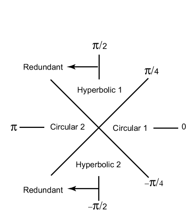
Figure 1: Forms of the $ABCD$ matrix depending on the angle $\theta.$

In this way, we can combine the four Wigner matrices into an exponential function of one analytic matrix. The problem is how to compute the exponential form of Eq.(8). Its Taylor expansion is

$$[abcd]=\sum_{n}\frac{r^{n}}{n!}[M(\theta)]^{n}.$$ (11)

This is an infinite series except at $\theta=\pm\pi/4$. If $\theta=45^{o}$, the $M$ matrix becomes

$$M=\pmatrix{0&0\cr\sqrt{2}&0}.$$ (12)

Since $M^{2}=0$, the series truncates. The $abcd$ matrix becomes

$$[abcd]=\pmatrix{1&0\cr r\sqrt{2}&1}.$$ (13)

Likewise, when $\theta=-\pi/4$,

$$[abcd]=\pmatrix{1&-r\sqrt{2}\cr 0&1}.$$ (14)

This aspect is illustrated in Fig. 1. The Taylor series truncates at $\theta=\pm\pi/4$. In the circular regions 1 and 2, $(\sin\theta)^{2}$ is smaller than $(\cos\theta)^{2}$. In the hyperbolic regions 1 and 2, $(\cos\theta)^{2}$ is smaller than $(\sin\theta)^{2}$.

Also in Fig. 1, the symmetry of trigonometry tells us the region $\pi/2<\theta<3\pi/2$ is redundant if we allow both positive and negative values of $r$ in Eq.(8). In this way, we restrict $\cos\theta$ to positive values. In circular region 1, $\sin\theta$ can be both positive or negative.

In the region $(\cos\theta)^{2}>(\sin\theta)^{2},$ and $|\theta|<\pi/4$, if $\sin\theta$ is positive, we can write the $M$ matrix as

$$M(\theta)=\sqrt{\cos(2\theta)}\pmatrix{0&-\exp{(-\eta)}\cr\exp{(\eta)}&0}.$$ (15)

with

$$\exp(-\eta)=\sqrt{\frac{\cos\theta-\sin\theta}{\cos\theta+\sin\theta}},$$ (16)

where $\eta$ is positive. This formula is valid also when $\sin\theta$ is negative, but $\eta$ is also negative. We now write $M(\theta)$ as

$$M(\theta)=\sqrt{\cos(2\theta)}\pmatrix{e^{-\eta/2}&0\cr 0&e^{\eta/2}}\pmatrix{0&-1\cr 1&0}\pmatrix{e^{\eta/2}&0\cr 0&e^{-\eta/2}}.$$ (17)

Then

$$\left(M(\theta)\right)^{n}=\left(\cos(2\theta)\right)^{n/2}\pmatrix{e^{-\eta/2}&0\cr 0&e^{\eta/2}}\pmatrix{0&-1\cr 1&0}^{n}\pmatrix{e^{\eta/2}&0\cr 0&e^{-\eta/2}}.$$ (18)

Thus

$$[abcd]=\pmatrix{e^{-\eta/2}&0\cr 0&e^{\eta/2}}\pmatrix{\cos\phi&-\sin\phi\cr\sin\phi&\cos\phi}\pmatrix{e^{\eta/2}&0\cr 0&e^{-\eta/2}},$$ (19)

which is

$$[abcd]=\pmatrix{\cos\phi&-e^{-\eta}\sin\phi\cr e^{\eta}\sin\phi&\cos\phi}$$ (20)

with

$$\phi=r\sqrt{\cos(2\theta)}.$$ (21)

In terms of the four parameters of the $ABCD$ matrix,

$$\cos\phi=\frac{A+B}{2},$$

$$e^{-2\eta}=\frac{-b}{c}=\frac{C-B-\sqrt{(B+C)^{2}+(A-D)^{2}}}{C-B+\sqrt{(B+C)^{2}+(A-D)^{2}}}.$$ (22)

where $\cos\phi$ is smaller than one, and $b$ is negative.

If $(\sin\theta)^{2}>(\cos\theta)^{2}$, or $\pi/4<|\theta|<\pi/2$, we have to consider two separate regions in Fig. 1, where $\cos\theta$ is positive, while $\sin\theta$ can take both positive and negative signs. $\cos(2\theta)$ is negative. The $M$ matrix should becomes

$$M(\theta)=\sqrt{-\cos(2\theta)}\pmatrix{0&\exp{(-\eta)}\cr\exp{(\eta)}&0}.$$ (23)

with

$$\exp(-\eta)=\sqrt{\frac{\sin\theta-\cos\theta}{\sin\theta+\cos\theta}},$$ (24)

for both positive and negative values $\sin\theta$, but $\eta$ is positive and is negative respectively.

Then the Taylor expansion leads to

$$[abcd]=\pmatrix{\cosh\chi&e^{-\eta}\sinh\chi\cr e^{\eta}\sinh\chi&\cosh\chi},$$ (25)

with

$$\chi=r\sqrt{-\cos(2\theta)}.$$ (26)

In terms of the parameters of the original $ABCD$ matrix,

$$\cosh\chi=\frac{A+B}{2},$$

$$e^{-2\eta}=\frac{b}{c}=\frac{B-C+\sqrt{(B+C)^{2}+(A-D)^{2}}}{C-B+\sqrt{(B+C)^{2}+(A-D)^{2}}}.$$ (27)

Here $\cosh\chi$ is greater than one, and both $b$ and $c$ are positive.

We can now go back to Eq.(16) and Eq.(24), and write $\tan\theta$ in terms of $\eta$. Then $\tan\theta$ becomes

$$\tan\theta=\frac{b+c}{c-b}=\frac{\sqrt{(A-D)^{2}+(B+C)^{2}}}{C-B},$$ (28)

for all values of $\theta$ between $-\pi/2$ and $\pi/2$. The parameter $r$ is

$$r=\left[\frac{b^{2}+c^{2}}{-2bc}\right]^{1/2}\phi,$$

$$r=\left[\frac{b^{2}+c^{2}}{2bc}\right]^{1/2}\chi,$$ (29)

for $(\sin\theta)^{2}<(\cos\theta)^{2}$ and $(\sin\theta)^{2}>(\cos\theta)^{2}$ respectively, with

$$\left[\frac{b^{2}+c^{2}}{2bc}\right]^{1/2}=\left[\frac{2\left(B^{2}+C^{2}\right)+(A-D)^{2}}{4BC+(A-D)^{2}}\right]^{1/2}.$$ (30)

Let us now look at how the transition of the $abcd$ from Eq. (20) to Eq. (25). This is a puzzling question because the matrix $M(\theta)$ remains analytic in the neighborhood of $\theta=\pi/4$ (see Fig. 1. In order to tackle this problem, we write $M(\theta)$ of Eq.(9) as

$$M(\theta)=(\cos\theta)\pmatrix{0&-(1-\tan\theta)\cr 1+\tan\theta&0}.$$ (31)

In the neighborhood of $\theta=\pi/4$, we can set $\cos\theta=1/\sqrt{2}$ and $(1+\tan\theta)=2$, and

$$M(\theta)=\frac{1}{\sqrt{2}}\pmatrix{0&-(1-\tan\theta)\cr 2&0}.$$ (32)

Then up to $r^{2}$, the Taylor leads to

$$[abcd]==\pmatrix{1-r^{2}(1-\tan\theta)/2&-r(1-\tan\theta)/\sqrt{2}\cr r\sqrt{2}&1-r^{2}(1-\tan\theta)/2}.$$ (33)

If $\theta$ is smaller than $\pi/4$, the diagonal elements of this matrix are smaller than $1$, like $\cos\phi$ in Eq.(20). If $\theta$ becomes greater than $\pi/4$, the diagonal element becomes greater than $1$ like $\cosh\chi$ in Eq.(25). If $\tan\theta=1$, the result becomes that of Eq.(13).

We can give a similar reasoning for the neighborhood of $\tan\theta=-1$. The Taylor expansion leads to

$$[abcd]=\pmatrix{1-r^{2}(1+\tan\theta)/2&-r\sqrt{2}\cr r(1+\tan\theta)/\sqrt{2}&1-r^{2}(1+\tan\theta)/2}.$$ (34)

leading to Eq.(14) for $\theta=-\pi/4.$

The exponential form given in Eq.(8) is very convenient when we study periodic systems where the $ABCD$ matrix is applied repeatedly. We shall return to this problem in Sec. 4.

3 Optical Activities

In his recent paper [2], one of the present authors used the two-by-two matrix formulation of optical activities applicable to the transverse electric field of an optical wave. The direction of the electric component rotates as the optical wave propagates. In the real world, the medium causes also an attenuation of the transverse components. This does not interfere with the rotational character. However, there is a problem if the dissipation coefficients are different for two perpendicular directions.

Let us start from a circularly polarized light wave which can be decomposed into the right-polarized and left polarized components. If they have different indexes of refraction, we can write the light wave as

$$\pmatrix{E_{x}\cr E_{y}}=\frac{1}{2}\pmatrix{1\cr i}\exp{\left\{i\left(k_{1}z-\omega t\right)\right\}}+\frac{1}{2}\pmatrix{1\cr-i}\exp{\left\{i\left(k_{2}z-\omega t\right)\right\}}$$ (35)

This two terms can be combined into

$$\pmatrix{E_{x}\cr E_{y}}=\pmatrix{\cos(\gamma z)\cr\sin(\gamma z)}\exp{\left\{i\left(kz-\omega t\right)\right\}},$$ (36)

with

$$k=\frac{1}{2}\left(k_{1}+k_{2}\right),\qquad\gamma=\frac{k_{1}-k_{2}}{2}.$$ (37)

If we start with a polarized light wave taking the form

$$\pmatrix{E_{x}\cr E_{y}}=\pmatrix{A\exp{\left\{i(kz-\omega t)\right\}}\cr 0},$$ (38)

the optical activity is carried out by the rotation matrix

$$R(\gamma z)=\pmatrix{\cos(\gamma z)&-\sin(\gamma z)\cr\sin(\gamma z)&\cos(\gamma z)}.$$ (39)

The optical ray is expected to be attenuated due to absorption by the medium. The attenuation coefficient in one transverse direction could be different from the coefficient along the other direction. Thus, if the rate of attenuation along the $x$ direction is different from that along $y$ axis, this asymmetric attenuation can be described by

$$\pmatrix{\exp{\left(-\mu_{1}z\right)}&0\cr 0&\exp{\left(-\mu_{2}z\right)}}=e^{-\lambda z}\pmatrix{\exp{(\mu z)}&0\cr 0&\exp{(-\mu z)}},$$ (40)

with

$$\lambda=\frac{\mu_{2}+\mu_{1}}{2},\qquad\mu=\frac{\mu_{2}-\mu_{1}}{2}.$$ (41)

The exponential factor $\exp{(-\lambda z)}$ is for the overall attenuation, and the matrix

$$\pmatrix{\exp{(\mu z)}&0\cr 0&\exp{(-\mu z)}}$$ (42)

performs a squeeze transformation. This matrix expands the $x$ component of the polarization, while contracting the $y$ component. We shall call this the squeeze along the $x$ direction.

The squeeze does not have to be along the $x$ and $y$directions For convenience, let us rotate the squeeze axis by $45^{o}$. Then the squeeze matrix becomes

$$S(\mu z)=\pmatrix{\cosh(\mu z)&\sinh(\mu z)\cr\sinh(\mu z)&\cosh(\mu z)}.$$ (43)

If this squeeze is followed by the rotation of Eq.(39), the net effect is

$$e^{-\lambda z}\pmatrix{\cos(\gamma z)&-\sin(\gamma z)\cr\sin(\gamma z)&\cos(\gamma z)}\pmatrix{\cosh(\mu z)&\sinh(\mu z)\cr\sinh(\mu z)&\cosh(\mu z)},$$ (44)

where $z$ is in a macroscopic scale, perhaps measured in centimeters. However, this is not an accurate description of the optical process.

This happens in a microscopic scale of $z/N$, and becomes accumulated into the macroscopic scale of $z$ after the $N$ repetitions, where $N$ is a very large number. We are thus led to the transformation matrix of the form

$$Z(\gamma,\mu,z)=\left[e^{-\lambda z/N}S(\mu z/N)R(\gamma z/N)\right]^{N}.$$ (45)

In the limit of large $N$, this quantity becomes

$$e^{-\lambda z}\left[\pmatrix{1&\mu z/N\cr\mu z/N&1}\pmatrix{1&-\gamma z/N\cr\gamma z/N&1}\right]^{N}.$$ (46)

Since $\gamma z/N$ and $\mu z/N$ are very small,

$$Z(\gamma,\mu,z)=e^{-\lambda z}\left[\pmatrix{1&0\cr 0&1}+\pmatrix{0&-\gamma+\mu\cr\gamma+\mu&0}\frac{z}{N}\right]^{N}.$$ (47)

For large $N$, we can write this matrix as [2]

$$Z(\gamma,\mu,z)=e^{-\lambda z}\exp{\left\{kzM(\theta)\right\}},$$ (48)

where the $M$ matrix is

$$M(\theta)=\pmatrix{0&-\cos\theta+\sin\theta\cr\cos\theta+\sin\theta&0},$$ (49)

with

$$k={\sqrt{\gamma^{2}+\mu^{2}}},$$

$$\cos\theta=\frac{\gamma}{\sqrt{\gamma^{2}+\mu^{2}}},$$

$$\sin\theta=\frac{\mu}{\sqrt{\gamma^{2}+\mu^{2}}}.$$ (50)

We note here that the $M(\theta)$ matrix of Eq.(49) is the same as that of Eq.(9) which determines the branch property of the $ABCD$ matrix. At this point, it is more convenient to work with $kM(\theta)$.

$$kM(\theta)=\pmatrix{0&-\gamma+\mu\cr\gamma+\mu&0}.$$ (51)

If $\gamma>\mu$, the $rM$ matrix can then be written as

$$kM=\sqrt{\gamma^{2}-\mu^{2}}\pmatrix{0&-e^{-\eta}\cr e^{\eta}&0},$$ (52)

where $\eta$ of Eq.(16) becomes

$$e^{-2\eta}=\sqrt{\frac{\gamma-\mu}{\gamma+\mu}}=\sqrt{\frac{\cos\theta-\sin\theta}{\cos\theta+\sin\theta}}.$$ (53)

Thus, the exponential function in Eq.(48) can be evaluated according to the procedure defined in Sec. 2. This expression is the same as that of Eq.(16).

The exponential form $\exp{(kzM)}$ in of Eq.(48) becomes

$$\pmatrix{e^{-\eta/2}&0\cr 0&e^{\eta/2}}\pmatrix{\cos(\gamma^{\prime}z)&-\sin(\gamma^{\prime}z)\cr\sin(\gamma^{\prime}z)&\cos(\gamma^{\prime}z)}\pmatrix{e^{\eta/2}&0\cr 0&e^{-\eta/2}},$$ (54)

where

$$\gamma^{\prime}=\sqrt{\gamma^{2}-\mu^{2}}.$$ (55)

The transformation matrix of Eq.(48) takes the form

$$Z(\gamma,\mu,z)=e^{-\lambda z}\pmatrix{\cos(\gamma^{\prime}z)&-e^{-\eta}\sin(\gamma^{\prime}z)\cr e^{\eta}\sin(\gamma^{\prime}z)&\cos(\gamma^{\prime}z)},$$ (56)

If $\mu>\gamma$, the $rM$ matrix becomes

$$kM=\sqrt{\mu^{2}-\gamma^{2}}\pmatrix{0&e^{-\eta}\cr e^{\eta}&0},$$ (57)

where $\eta$ of Eq.(24) takes the form

$$e^{-2\eta}=\sqrt{\frac{\mu-\gamma}{\mu+\gamma}}=\sqrt{\frac{\sin\theta-\cos\theta}{\cos\theta+\sin\theta}},$$ (58)

and $Z$ becomes

$$Z(\gamma,\mu,z)=e^{-\lambda z}\pmatrix{\cosh(\mu^{\prime}z)&e^{-\eta}\sinh(\mu^{\prime}z)\cr e^{\eta}\sinh(\mu^{\prime}z)&\cosh(\mu^{\prime}z)},$$ (59)

where

$$\mu^{\prime}=\sqrt{\mu^{2}-\gamma^{2}}.$$ (60)

In this section, we discussed a system of optical activities with asymmetric dissipation as a physical illustration of the mathematical procedure discussed in Sec. 2. We have already seen that $M(\theta)$ of Eq.(49) has the same form as that of Eq.(9), and that angle $\theta$ can be defined in terms of the parameters $\gamma$ and $\mu$, as shown in Eq.(3). The parameter $\eta$ can also be defined in terms of $\gamma$ and $\mu$, and its expression is the same as the one given in terms of the angle $\theta$.

As for the branches, we note that both $\gamma$ and $\mu$ can be negative and positive. Thus, the angle $\theta$ can cover the entire range from zero to $2\pi$. We can write $\gamma^{\prime}$ and $\mu^{\prime}$ as

$$\gamma^{\prime}=k\sqrt{\cos^{2}\theta-\sin^{2}\theta},\qquad\mu^{\prime}=k\sqrt{\sin^{2}\theta-\cos^{2}\theta}.$$ (61)

Since $\cos^{2}\theta-\sin^{2}\theta=\cos(2\theta),$ $\gamma^{\prime}z$ and $\mu^{\prime}z$ correspond to $\phi$ and $\chi$ of Eq.(21) and Eq.(26) respectively.

If we start with $\mu=0$, it is simply a rotation of the transverse component of the electric field and the overall attenuation factor is $\exp{(-\lambda z)}$. The rate of this rotation decreased as $\mu$ increases, and the rotation stops at $\gamma=\mu$. For $\mu>\gamma$, there are no rotations. It would be very interesting to test these effects experimentally.

We should not forget the fact that the equi-diagonal $[abcd]$ matrix is a rotated $ABCD$ matrix. The rotation matrix is given in Eq.(5). This rotation changes the optical ray of Eq.(36) to

$$\pmatrix{E_{x}\cr E_{y}}=\pmatrix{\cos(\gamma z+\alpha/2)\cr\sin(\gamma z+\alpha/2)}\exp{\left\{i\left(kz-\omega t\right)\right\}}.$$ (62)

This is also an observable effect.

We have seen in this section that the asymmetric optical activity can serve as an analog computer for the mathematical procedure given in Sec. 2 which is in fact an alternative to the diagonalization of the $ABCD$ matrix.

4 Periodic Systems in Optics

Let us summarize what we can do about the $ABCD$ matrix.

• We should first rootate to an equi-diagonal matrix [abcd].

• If the diagonal elements of this equi-diagonal matrix are smaller than one, it can be written as

  $$\pmatrix{\cos\phi&-e^{-\eta}\sin\phi\cr e^{\eta}\sin\phi&\cos\phi},$$ (63)

  with $\exp{(-\eta)}=-b/c$, which can also be written in terms of the elements of the original $ABCD$ matrix, as shown in Eq. (21).

• If the diagonal elements of the equi-diagonal matrix are greater than than one, the matrix can be written as

  $$\pmatrix{\cosh\chi&e^{-\eta}\sinh\chi\cr e^{\eta}\sinh\chi&\cosh\chi},$$ (64)

  with $\exp{(-\eta)}=b/c$, which takes the form of Eq.(26) in terms of the elements of the $ABCD$ Matrix.

• If one of the off-diagonal elements vanish, the diagonal elements have to be one.

• It is possible to combine all these cases into one exponential function of one analytic matrix. It can be written as

  $$[abcd]=\exp{\left\{r\pmatrix{0&-\cos\theta+\sin\theta\cr\cos\theta+\sin\theta&0}\right\}}.$$ (65)

• When $\theta=\pm\pi/4,$ the Taylor series truncates, and

  $$[abcd]=\pmatrix{1&-r(1\mp 1)/\sqrt{2}\cr r(1\pm 1)/\sqrt{2}&1}.$$ (66)

4.1 Laser Cavities

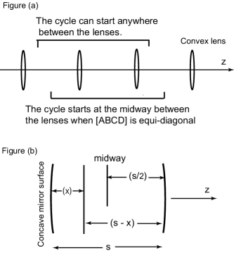
Figure 2: Optical rays in a laser cavity. (a) Multiple cycles in a laser cavity are equivalent to the beam going through multiple lenses, for which one cavity cycle corresponds to the propagation of light through a sub-system of two lenses. The $ABCD$ matrix becomes equi-diagonal when the cycle begins at the midway between the lenses. (b) A laser cavity consisting of two concave mirrors with separation $s$.

A laser cavity consists of two concave mirrors separated by distance $s$ as illustrated in Fig. 2. The mirror matrix takes the form

$$\pmatrix{1&0\cr-2/R&1},$$ (67)

where $R$ is the radius of the concave mirror. The separation matrix is

$$\pmatrix{1&s\cr 0&1}.$$ (68)

If we start the cycle from one of the two mirrors one complete cycle consists of

$$\pmatrix{1&0\cr-2/R&1}\pmatrix{1&s\cr 0&1}\pmatrix{1&0\cr-2/R&1}\pmatrix{1&s\cr 0&1}.$$ (69)

If we start the beam at the position $x$ from the mirror, then one complete cycle becomes

$$\pmatrix{1&x\cr 0&1}\pmatrix{1&0\cr-2/R&1}\pmatrix{1&s-x\cr 0&1}$$

$$\hskip 56.9055pt\times\pmatrix{1&x\cr 0&1}\pmatrix{1&0\cr-2/R&1}\pmatrix{1&s-x\cr 0&1}.$$ (70)

This cycle consist of two identical half cycles.

Thus, we shall use the half-cycle matrix as our starting point. Then the half-cycle $ABCD$ matrix becomes

$$[ABCD]=\pmatrix{1&x\cr 0&1}\pmatrix{1&0\cr-2/R&1}\pmatrix{1&s-x\cr 0&1},$$ (71)

It is now possible to replace replace $R$ and $x$ and by $R/s$ and $x/s$ respectively and set $s=1$ [1]. Then

$$[ABCD]=\pmatrix{1-2xf&1-2xf(1-x)\cr-2f&1-2f(1-x)},$$ (72)

where $f=s/R$, and is expected to be a small number because the mirror radius $R$ is much larger than the separation of the mirrors.

It can be brought to an equi-diagonal form by a rotation as given in Eq.(4). According to Eq.(2), the rotation angle is

$$\tan\alpha=\frac{2f(2x-1)}{1-2f\left(1+x-x^{2}\right)}.$$ (73)

This angle is zero when $x=1/2$. In this case, the laser cycle starts at the midway between the lenses [1]. Then the $ABCD$ matrix becomes

$$[abcd]=\pmatrix{1-f&1-f/2\cr-2f&1-f},$$ (74)

This matrix can then be written as

$$[abcd]=\pmatrix{\cos\phi&e^{\eta}\sin\phi\cr-e^{-\eta}\sin\phi&\cos\phi}.$$ (75)

with

$$\cos\phi=1-f,\qquad e^{2\eta}=\frac{2-f}{4f}.$$ (76)

This is the result we obtained in our earlier paper on laser cavities [5], where the cycle starts from the midway between the lenses. The signs of $\phi$ and $\eta$ are opposite to those given in Eq.(20), but this is purely for convenience. There are no fundamental problems.

We can now write this expression in an exponential form

$$[abcd]=\exp{\left\{r\pmatrix{0&\cos\theta+\sin\theta\cr-\cos\theta+\sin\theta&0}\right\}},$$ (77)

with

$$\tan\theta=\frac{2-5f}{2+3f},$$

$$r=\left[\frac{13f-17f^{2}}{8-17f^{2}}\right]^{1/2}\phi,$$ (78)

where $\phi$ is given in Eq.(76). Since the radius of the mirror is much larger than the mirror separation, $f$ is a small number, and $\tan\theta$ is close to one and $r$ is a small number.

The $N$-cycle laser consists of $2N$ half-cycles, and its $abcd$ matrix is

$$[abcd]^{2N}=\exp{\left\{2Nr\pmatrix{0&\cos\theta+\sin\theta\cr-\sin\theta+\cos\theta&0}\right\}}.$$ (79)

This section is a straight-forward application of the procedure given in Sec. 2. We know that $\sin(r\theta)^{2N}$ is not $\sin(2Nr\theta)$, but the exponential form gives us the convenience of $[\exp{(ir\theta)}]^{2N}=\exp{(i2Nr\theta)}.$ We have given a two-by-two matrix formulation of this convenience applicable to the $ABCD$ matrix.

4.2 Multilayer Optics

From the physical concept of Wigner’s little group whose transformations leave the four-momentum of a given particle invariant [3, 4], it has been established in the literature that [6]

$$S(\eta)WS(-\eta)=R(\xi)B(-2\lambda)R(\xi),$$ (80)

where $W$ is one of the four Wigner matrices given in Eq.(1), $R(\xi)$ is the rotation matrix of the form of Eq.(5), and

$$S(\eta)=\pmatrix{e^{\eta/2}&0\cr 0&e^{-\eta/2}},$$

$$B(\lambda)=\pmatrix{\cosh(\lambda/2)&\sinh(\lambda/2)\cr\sinh(\lambda/2)&\cosh(\lambda/2)},$$ (81)

and the continuous parameters $\xi$ and $\lambda$ take care of the four different Wigner parameters. These parameters can be written in terms of $\eta$ and the parameter of the Wigner matrix, as shown in Ref. [1, 6].

Since the left side of Eq.(80) can be written as an exponential form, we can write

$$R(\xi)B(-2\lambda)R(\xi)=\exp{\left\{r\pmatrix{0&-\cos\theta+\sin\theta\cr\cos\theta+\sin\theta&0}\right\}},$$ (82)

where $r$ and $\theta$ are also continuous variables.

Figure 3: Multilayer consisting of two different refractive indices. One complete cycle starts at the boundary between medium 2 and medium 1.

With this mathematical preparation, let us study multilayer optics. In this branch of optics, we have to consider the $ABCD$ matrix applicable to two beams moving in opposite directions, one which is the incident beam and the other is the reflected beam [7]. We can represent them as a two component column matrix

$$\pmatrix{E_{+}e^{ikz}\cr E_{-}e^{-ikz}},$$ (83)

where the upper and lower components correspond to the incoming and reflected beams respectively. For a given frequency, the wave number depends on the index of the refraction. Thus, if the beam travels along the distance $d$, the column matrix should be multiplied by the two-by-two matrix [7]

$$P(\beta_{j})=\pmatrix{e^{i\beta_{j}/2}&0\cr 0&e^{-i\beta_{j}/2}},$$ (84)

where $\beta_{j}/2=k_{j}d$ and $j$ is denoting each different medium. If the beam propagates along the first medium and meets the boundary at the second medium, it will be partially reflected and partially transmitted. The boundary matrix is [7]

$$B(\nu)=\pmatrix{\cosh(\nu/2)&\sinh(\nu/2)\cr\sinh(\nu/2)&\cosh(\nu/2)},$$ (85)

with

$$\cosh(\nu/2)=1/t_{12},\qquad\sinh(\nu/2)=r_{12}/t_{12},$$ (86)

where $t_{12}$ and $r_{12}$ are the transmission and reflection coefficients respectively, and they satisfy $\left(r_{12}^{2}+t_{12}^{2}\right)=1.$ The boundary matrix for the second to first medium is the inverse of the above matrix. Therefore, one complete cycle, starting from the second medium, consists of

$$B(\nu)P(\beta_{1})B(-\nu)P(\beta_{2}),$$ (87)

as illustrated in Fig. 3. This complex-valued matrix can be cast into a real matrix by a similarity transformation with the transformation matrix

$$C=\frac{1}{\sqrt{2}}\pmatrix{e^{i\pi/4}&e^{i\pi/4}\cr-e^{-i\pi/4}&e^{-i\pi/4}},$$ (88)

This transforms the boundary matrix $B(\nu)$ of Eq.(85) to a squeeze matrix $S(\nu)$ of Eq.(4.2), and the phase shift matrices $P(\beta_{j})$ of Eq.(84) to rotation matrices $R(\beta_{j})$ of the form given in Eq.(5). We are thus led to consider the $ABCD$ matrix of the form

$$[ABCD]=S(\nu)R(\beta_{1})S(-\nu)R(\beta_{2}).$$ (89)

If $W$ in Eq.(80) is a rotation matrix, we can write

$$S(\nu)R(\beta_{1})S(-\nu)=R(\xi_{1})B(-2\lambda)R(\xi_{1})$$ (90)

where

$$\cosh\lambda=(\cosh\nu)\sqrt{1-\cos^{2}(\beta_{1}/2)\tanh^{2}\nu},$$ (91)

$$\cos\xi_{1}=\frac{\cos(\beta_{1})}{(\cosh\nu)\sqrt{1-\cos^{2}(\beta_{1}/2)\tanh^{2}\nu}}.$$ (92)

The $ABCD$ matrix can then be simplified to

$$[ABCD]=R(\xi_{1})B(-2\lambda)R(\xi_{2})$$ (93)

with

$$\xi_{2}=\xi_{1}+\beta_{2}$$ (94)

It is now possible to write the above form as

$$[ABCD]=R(\alpha)[R(\xi)B(-2\lambda)R(\xi)]R(-\alpha),$$ (95)

with

$$\xi=\frac{1}{2}\left(\xi_{1}+\xi_{2}\right),\qquad\alpha=\frac{1}{2}\left(\xi_{1}-\xi_{2}\right).$$

The role of the rotation matrix $R(\alpha)$ matrix is clearly defined in Sec. 2. Thus $R(\xi)B(-2\lambda)R(\xi)$ is the equi-diagonal matrix, and

$$R(\xi)B(-2\lambda)R(\xi)=\pmatrix{\cosh\lambda\cos\xi&-(\sin\xi\cosh\lambda+\sinh\lambda)\cr\sin\xi~{}\cosh\lambda-\sinh\lambda&\cosh\lambda~{}\cos\xi}.$$ (96)

Thus, if $(\cosh\lambda\cos\xi)$ is smaller than one, we can write this matrix as

$$\pmatrix{\cos\phi&-e^{\eta}\sin\phi\cr e^{-\eta}\sin\phi&\cos\phi},$$ (97)

with

$$\cos\phi=(\cosh\lambda)\cos\xi,\qquad e^{2\eta}=\frac{(\cosh\lambda)\sin\xi+\sinh\lambda}{(\cosh\lambda)\sin\xi-\sinh\lambda}.$$ (98)

Thus, if $(\cosh\lambda\cos\xi)$ is greater than one, we should write the equi-diagonal matrix as

$$\pmatrix{\cosh\chi&-e^{\eta}\sinh\chi\cr-e^{-\eta}\sinh\chi&\cosh\chi},$$ (99)

with

$$\cosh\chi=(\cosh\lambda)\cos\xi,\qquad e^{2\eta}=\frac{\sinh\lambda+(\cosh\lambda)\sin\xi}{\sinh\lambda-(\cosh\lambda)\sin\xi}.$$ (100)

We are now interested in the exponential form

$$R(\xi)B(-2\lambda)R(\xi)=\exp{\left\{r\pmatrix{0&-(\cos\theta+\sin\theta)\cr\cos\theta-\sin\theta&0}\right\}}.$$ (101)

with

$$\tan\theta=\frac{\tanh\lambda}{\sin\xi}.$$ (102)

As for the $r$ parameter,

$$r=\left[\frac{\sin^{2}\xi+\tanh^{2}\lambda}{\sin^{2}\xi-\tanh^{2}\lambda}\right]^{1/2}\phi,\quad r=\left[\frac{\sin^{2}\xi+\tanh^{2}\lambda}{\tanh^{2}\lambda-\sin^{2}\xi}\right]^{1/2}\chi,$$ (103)

for $(\cosh\lambda\cos\xi)<1$, and for $(\cosh\lambda\cos\xi)>1$, respectively.

In this section, we started with two media with two different indexes of refraction, corresponding to two rotation matrices $R\left(\beta_{1}\right)$ and $R\left(\beta_{2}\right)$ given in Eq.(89) respectively. However, the combined effect in not necessarily a rotation matrix. It can be analytically continued to the hyperbolic branch through the exponent of the $ABCD$ matrix.

When $(\cosh\lambda\cos\xi)^{2}=1$, one of the off-diagonal elements in Eq.(101) vanishes, and this case was repeatedly discussed in the literature [1, 6], also in the present paper.

Concluding Remarks

In this paper, we noted first that the two-by-two $ABCD$ matrix can be represented as a similarity transformation of one of the four matrices which we choose to call the Wigner matrices. We then combined these Wigner matrices into one exponential form of an analytic matrix.

While $\cos\phi$ and $\cosh\chi$ correspond to a circle and a hyperbola respectively, the lines in Fig. 1 correspond parabolas in the four-dimensional representation of the Lorentz group [3, 8]. Ancient Greeks used a circular cone to combine these curves into one. This is the reason why we call them conic sections. It is gratifying to note that the optical devices we discussed in Secs. 3 and 4 can play the role of a conic section. Instead of three-dimensional cone, we used a two-dimensional plane in Fig. 1.

We have seen in this paper that Taylor expansion of this analytic form results in four branches. How does this happen? Let us go to the Taylor expansion of Eq.(11). This infinite series truncates at $(\sin\theta)^{2}=(\cos\theta)^{2}$ or along the two lines in Fig. 1. We are not familiar with mathematical singularities resulting from the truncation of the infinite Taylor series. This appears to be an interesting problem in mathematics, but it is beyond the scope of this paper.

References

• [1] S. Başkal and Y. S. Kim, J. Opt. Soc. Am. A 26, 3049-2054 (2009).
• [2] Y. S. Kim, J. Mod. Opt. 57, 17-22 (2010).
• [3] E. Wigner, Ann. Math. 40, 149-204 (1939).
• [4] Y. S. Kim and M. E. Noz, Theory and Applications of the Poincaré Group (Reidel, Dordrecht, 1986).
• [5] S. Başkal and Y. S. Kim, Phys. Rev. E 66, 026604-026609 (2002).
• [6] E. Georgieva and Y. S. Kim, Phys. Rev. E 68, 026606: 1-6 (2003).
• [7] R. M. A. Azzam and N. M. Bashara, Ellipsometry and Polarized Light (Elsevier, Amsterdam, 1977).
• [8] Y. S. Kim and E. P. Wigner, J. Math. Phys. 31, 55-60 (1990).