Light-front quark distributions in the nucleon and nucleon electromagnetic form factors

Abstract

Longitudinal and transverse quark momentum distributions in the nucleon are calculated from a phenomenological quark-nucleon vertex function obtained through an investigation of the nucleon electromagnetic form factors within a light-front framework.

1 INTRODUCTION

A wealth of information on the partonic structure of the nucleon is encoded in the generalized parton distributions (GPD’s) and extensive research programs are being pursued to gain information on nucleon GPD’s.

Our strategy to this end is to determine the quark-nucleon vertex function from an investigation of nucleon electromagnetic (em) form factors within the light-front dynamics, and then to use the obtained vertex function to evaluate the nucleon GPD’s. Indeed, light-front dynamics opens a unique possibility to study the hadronic state in both the valence and the nonvalence sector [1], since within a light-front framework no spontaneous pair production occurs and a meaningful Fock state expansion is possible :

$$|baryon\rangle={|qqq\rangle}+{|qqq~{}q\bar{q}\rangle+|qqq~{}g\rangle.....}$$ (1)

As a first step, in this contribution we present our preliminary results for the unpolarized longitudinal and transverse parton momentum distributions in the nucleon.

2 NUCLEON VERTEX FUNCTION AND NUCLEON ELECTROMAGNETIC FORM FACTORS

We describe the quark-nucleon vertex function through a Bethe-Salpeter amplitude (BSA), whose Dirac structure is suggested by an effective Lagrangian [2]. Then the symmetrized BSA for the nucleon is approximated as follows

$$\Phi^{\sigma}_{N}(k_{1},k_{2},k_{3},P)=$$

$$\imath\left[~{}S(k_{1})~{}\tau_{y}~{}\gamma^{5}~{}S_{C}(k_{2})C~{}\otimes~{}S(k_{3})~{}+~{}\right.$$

$$S(k_{3})~{}\tau_{y}~{}\gamma^{5}~{}S_{C}(k_{1})C~{}\otimes~{}S(k_{2})~{}+$$

$$\left.~{}S(k_{3})~{}\tau_{y}~{}\gamma^{5}~{}S_{C}(k_{2})C~{}\otimes~{}S(k_{1})\right]$$

$$\times~{}~{}\Lambda(k_{1},k_{2},k_{3})~{}\chi_{\tau_{N}}~{}U_{N}(P,\sigma)$$ (2)

where $S(k)$ is the constituent quark (CQ) free propagator, $S_{C}(k)$ the charge conjugated propagator, $\Lambda(k_{1},k_{2},k_{3})$ describes the symmetric momentum dependence of the vertex function upon the quark momentum variables, $k_{i}$, $U_{N}(P,\sigma)$ is the nucleon spinor and $\chi_{\tau_{N}}$ the isospin eigenstate.

The matrix elements of the macroscopic current in the spacelike (SL) region are approximated microscopically by the Mandelstam formula [3]

$$\langle\sigma^{\prime},P^{\prime}|j^{\mu}~{}|P,\sigma\rangle=~{}3~{}N_{c}~{}\times$$

$$\int{d^{4}k_{1}\over(2\pi)^{4}}\int{d^{4}k_{2}\over(2\pi)^{4}}~{}{\Large{\Sigma}}\left\{\bar{\Phi}^{\sigma^{\prime}}_{N}(k_{1},k_{2},k^{\prime}_{3},P^{\prime})\right.~{}\times$$

$$\left.S^{-1}(k_{1})~{}S^{-1}(k_{2})~{}{\cal I}^{\mu}(k_{3},q)~{}\Phi^{\sigma}_{N}(k_{1},k_{2},k_{3},P)\right\}$$ (3)

where $N_{c}$ is the number of colors, $k^{\prime}_{3}=k_{3}+q$, and ${\cal I}^{\mu}(k_{3},q)$ is the quark-photon vertex. An analogous expression holds in the timelike (TL) region.

We adopt a Breit reference frame where $~{}~{}{\bf q}_{\perp}=0$ and $q^{+}=q^{0}+q^{3}=|q^{2}|^{1/2}$. Our CQ mass is  $m=m_{u}=m_{d}=200~{}MeV$.

The Mandelstam Formula is projected out by an analytic integration on $k_{1}^{-}$ and $k_{2}^{-}$, taking into account only the poles of the propagators. Then the current becomes the sum of a purely valence contribution (diagram (a) in Fig. 1) and a nonvalence (NV), pair-production contribution (diagram (b) in Fig. 1). Clearly, after the $k^{-}$ integrations, the vertex functions depend only upon the light-front three-momentum.

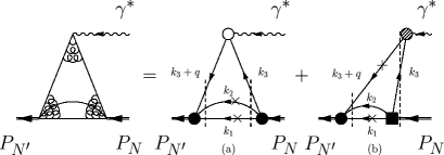
Figure 1: Diagrams for the SL nucleon current: (a) valence (triangle) contribution with $0<k_{i}^{+}<P^{+}$, and $~{}0\leq k_{3}^{+}+q^{+}<{P^{\prime}}^{+}$; (b) nonvalence, pair-production contribution with $0>k_{3}^{+}\geq-q^{+}$. A cross indicates a quark on the $k^{-}$-shell, i.e. $k^{-}=k^{-}_{on}=(m^{2}+k^{2}_{\perp})/k^{+}$. Solid circles and solid square represent valence and NV vertex functions, respectively (after Ref. [4]).

The quark-photon vertex has isoscalar and isovector contributions

$${\cal I}^{\mu}=~{}{\cal I}^{\mu}_{IS}+\tau_{z}{\cal I}^{\mu}_{IV}$$ (4)

and each term in Eq. (4) contains a purely valence contribution (in the SL region only) and a contribution corresponding to the pair production (Z-diagram). In turn the Z-diagram contribution can be decomposed in a bare term $+$ a Vector Meson Dominance (VMD) term (according to the decomposition of the photon state in bare, hadronic [and leptonic] contributions), viz

$${\cal I}^{\mu}_{i}(k,q)={\cal N}_{i}~{}\theta(P^{+}-k^{+})\theta(k^{+})\gamma^{\mu}+\theta({q}^{+}+k^{+})$$

$$\times~{}\theta(-k^{+})~{}\left\{Z_{B}~{}{\cal N}_{i}~{}\gamma^{\mu}+Z^{i}_{VM}~{}\Gamma^{\mu}[k,q,i]\right\}$$ (5)

with $i=IS,IV$, ${\cal N}_{IS}=1/6$ and ${\cal N}_{IV}=1/2$. The constants $Z_{B}$ (bare term) and $Z^{i}_{VM}$ (VMD term) are unknown weights to be extracted from the phenomenological analysis of the data.

According to $i$, the VMD term $\Gamma^{\mu}[k,q,i]$ includes isovector or isoscalar mesons. Indeed in [4] we extended to isoscalar mesons the microscopic model for the VMD successfully used in [5] for the pion form factor in the SL and in the TL region and based on the meson mass operator of Ref. [6]. As explained in [4], $\Gamma^{\mu}[k,q,i]$ does not involve free parameters. We consider up to 20 mesons for achieving convergence at high $|q^{2}|$.

In the valence vertexes (solid circles in Fig. 1) the spectator quarks are on the $k^{-}$-shell, and the BSA momentum dependence is approximated through a nucleon wave function a la Brodsky (PQCD inspired), namely

$$\Psi_{N}(\tilde{k}_{1},\tilde{k}_{2},P)=P^{+}~{}{{\Lambda}(k_{1},k_{2},k_{3})|_{(k_{1on}^{-},k_{2on}^{-})}\over[m_{N}^{2}-M^{2}_{0}(1,2,3)]^{~{}}}=$$

$$=~{}P^{+}~{}{\cal{N}}~{}{~{}(9~{}m^{2})^{7/2}\over(\xi_{1}\xi_{2}\xi_{3})^{p}~{}\left[\beta^{2}+M^{2}_{0}(1,2,3)\right]^{7/2}}~{}$$ (6)

where $\tilde{k}_{i}\equiv(k_{i}^{+},{\bf k}_{i\perp})$, $M_{0}(1,2,3)$ is the free mass of the three-quark system, $\xi_{i}=k^{+}_{i}/P^{+}$  ($i=1,2,3$) and ${\cal N}$ a normalization constant.

The power $7/2$ and the parameter $p=0.13$ are chosen to have an asymptotic decrease of the triangle contribution faster than the dipole.

Only the triangle diagram determines the magnetic moments, which are weakly dependent on $p$. Then $\beta=0.645$ can be fixed by the magnetic moments and we obtain $\mu_{p}=2.87\pm 0.02$   ($\mu_{p}^{exp}$ = 2.793) and $\mu_{n}=-1.85\pm 0.02$   ($\mu_{n}^{exp}$ = -1.913).

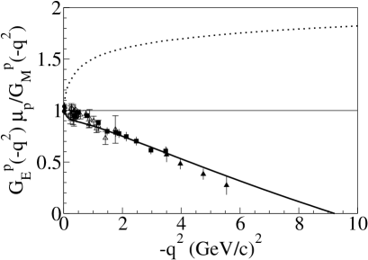
Figure 2: Ratio between electric and magnetic form factors for the proton vs $-q^{2}$. Solid line: full calculation, sum of triangle and pair-production terms; dotted line: triangle contribution only (after Ref. [4]).

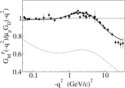
Figure 3: Magnetic proton form factor vs $-q^{2}$. Solid and dotted lines as in Fig. 2. $G_{D}(|q^{2}|)=[1+|q^{2}|/(0.71$ (GeV/c)${}^{2}]^{-2}$ (after Ref. [4]).

For the Z-diagram contribution, the NV vertex (solid square in Fig. 1) is needed. It can depend on the available invariants, i.e. on the free mass, $M_{0}(1,2)$, of the (1,2) quark pair and on the free mass, $M_{0}(N,\bar{3})$, of the ( nucleon - quark $\bar{3}$ ) system entering the NV vertex. Then in the SL region we approximate the momentum dependence of the NV vertex ${\Lambda}_{NV}^{SL}={\Lambda}(k_{1},k_{2},k_{3})|_{k^{-}_{1on},k^{{}^{\prime}-}_{3on}}$ by

$${\Lambda}_{NV}^{SL}=[g_{12}]^{2}[g_{N\bar{3}}]^{3/2}\left[{k_{12}^{+}\over P^{\prime+}}\right]\left[P^{\prime+}\over k_{\overline{3}}^{+}\right]^{r}\left[P^{+}\over k_{\overline{3}}^{+}\right]^{r}$$ (7)

with

$$k_{12}^{+}=k_{1}^{+}+k_{2}^{+}~{}~{}\quad g_{AB}={(m_{A}~{}m_{B})\over\left[\beta^{2}+M^{2}_{0}(A,B)\right]}$$ (8)

The power 2 of $[g_{12}]^{2}$ is suggested from counting rules. The power 3/2 of $[g_{N\bar{3}}]^{3/2}$ and the parameter $r=0.17$ are chosen to have an asymptotic dipole behavior for the NV contribution.

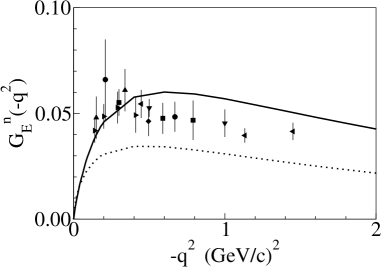
Figure 4: Electric neutron form factor vs $-q^{2}$. Solid and dotted lines as in Fig. 2 (after Ref. [4]).

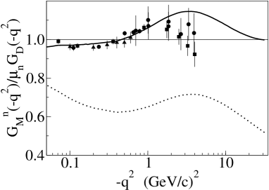
Figure 5: The same as in Fig. 3, but for the neutron (after Ref. [4]).

Analogous expressions with the same parameters are used for the nonvalence vertexes in the TL region (see Ref. [4] for the explicit expressions).

We perform a fit of our free parameters, $Z_{B}$, $Z^{i}_{VM}$, $p$, $r$ in the SL region and obtain the form factors shown in Figs. 2 - 5, with a $\chi^{2}$/datum = 1.7. As a result the weights for the pair-production terms are $Z_{B}=Z_{VM}^{IV}=2.283$ and $Z_{VM}^{IS}/Z_{VM}^{IV}=1.12$, remarkably close to one. The same values of our weight parameters are adopted to evaluate the TL form factors shown in Figs. 6 and 7.

Preliminary results of our model for the nucleon form factors were presented in [7].

The Z-diagram turns out to be essential for the description of the form factors in our reference frame with $q^{+}>0$. In particular the possible zero in $G_{E}^{p}/G_{M}^{p}$ is strongly related to the pair-production contribution.

In the TL region our parameter free calculations give a fair description of the proton data, apart for some missing strength at $q^{2}=4.5$ (GeV/c)²   and   $q^{2}=8$ (GeV/c)² (as occurs for the pion case [5]), which one could argue to be due to possible unknown vector mesons, missing in the spectrum of Ref. [6].

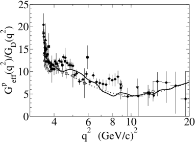
Figure 6: Proton effective form factor $G^{p}_{eff}(q^{2})/G_{D}(q^{2})$ in the timelike region vs $q^{2}$. Solid line: bare + VMD; dotted line: bare term. $G_{eff}(q^{2})=[(|G_{M}(q^{2})|^{2}~{}-~{}\eta~{}|G_{E}(q^{2})|^{2})/(1~{}-~{}\eta)]^{0.5}$ with $\eta=-2m_{N}^{2}/q^{2}$ (after Ref. [4]).

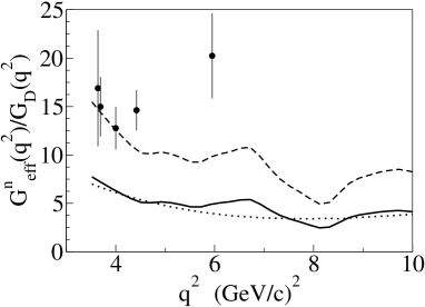
Figure 7: The same as in Fig. 5, but for the neutron. Dashed line: solid line arbitrarily multiplied by 2 (after Ref. [4]).

3 LONGITUDINAL AND TRANSVERSE QUARK MOMENTUM DISTRIBUTIONS IN THE NUCLEON

The longitudinal distribution $q(x)$ is the limit in the forward case, $P^{\prime}=P$, of the unpolarized generalized parton distribution ${H}^{q}(x,\xi,t)$. Indeed one can define the distributions ${H}^{q}(x,\xi,t)$ and $E^{q}(x,\xi,t)$ for the quark $q$ through the following relation

$$\frac{1}{2P^{+}}\bar{u}(P^{\prime},\lambda^{\prime})\left[{H}^{q}~{}\gamma^{+}+{E}^{q}~{}\imath\frac{\sigma^{+\alpha}q_{\alpha}}{2M}\right]{u}(P,\lambda)=$$

$$\int\frac{dz^{-}}{4\pi}e^{ix{\cal{P}}^{+}z^{-}}\left.\langle P^{\prime},\lambda^{\prime}|\bar{\psi}_{q}(-\frac{z}{2})\gamma^{+}\,\psi_{q}(\frac{z}{2})|P,\lambda\rangle\right|_{\tilde{z}=0}$$

where $\lambda$ is the nucleon helicity, $\tilde{z}\equiv\{z^{+},{\bf z}_{\perp}\}$ , $\psi_{q}(z)$ is the quark field isodoublet, while

$${\cal{P}}=\frac{1}{2}(P^{\prime}+P)\;\;\quad\quad t=(P^{\prime}-P)^{2}$$ (9)

$$\xi=-\frac{P^{\prime+}-P^{+}}{2{\cal{P}}^{+}}\quad\quad x=\frac{k^{+}}{{\cal{P}}^{+}}$$ (10)

and $k$ is the average momentum of the quark that interacts with the photon, i.e.

$$k=\frac{k_{3}+(k_{3}+q)}{2}$$ (11)

For $P^{\prime}=P$, both $q^{+}$ and $\xi$ are vanishing and $x=k_{3}^{+}/P^{+}=\xi_{3}$ coincides with the fraction of the longitudinal momentum carried by the active quark, i.e., with the Bjorken variable. As a consequence the function ${H}^{q}(x,\xi,t)$ reduces to the longitudinal parton distribution function $q(x)$ :

$${H}^{q}(x,0,0)=q(x)=\int d{\bf k}_{\perp}~{}~{}f_{1}^{q}(x,k_{\perp})=$$ (12)

$$\int\frac{dz^{-}}{4\pi}e^{ixP^{+}z^{-}}\left.\langle P|\bar{\psi}_{q}(-{z\over 2})\gamma^{+}\,\psi_{q}({z\over 2})|P\rangle\right|_{\tilde{z}=0}$$

where an average on the nucleon helicities is understood.

Once all the parameters of the nucleon light-front wave function $\Psi_{N}(\tilde{k}_{1},\tilde{k}_{2},P)$ have been determined, one can easily define the transverse-momentum-dependent distributions of the active quark in terms of the nucleon light-front wave function :

$$f_{1}^{u}(x,k_{\perp})=-{9~{}N_{c}\over 32~{}(2\pi)^{6}}~{}{1\over P^{+2}}~{}\times~{}$$

$$\int^{1-x}_{0}d\xi_{2}{1\over(1-x-\xi_{2})\xi_{2}}{1\over x^{2}}\int d{\bf k}_{2\perp}\left.{\cal H}_{u}\right|_{(k^{-}_{1on},k^{-}_{2on})}$$

$$\times~{}|\Psi_{N}(P^{+}~{}\xi_{1},{\bf k}_{1\perp},P^{+}~{}\xi_{2},{\bf k}_{2\perp},P)|^{2}$$ (13)

$$f_{1}^{d}(x,k_{\perp})={9~{}N_{c}\over 8~{}(2\pi)^{6}}~{}{1\over P^{+2}}~{}\times~{}$$

$$\int^{1-x}_{0}d\xi_{2}{1\over(1-x-\xi_{2})\xi_{2}}{1\over x^{2}}\int d{\bf k}_{2\perp}\left.{\cal H}_{d}\right|_{(k^{-}_{1on},k^{-}_{2on})}$$

$$\times~{}|\Psi_{N}(P^{+}~{}\xi_{1},{\bf k}_{1\perp},P^{+}~{}\xi_{2},{\bf k}_{2\perp},P)|^{2}~{}~{}\quad$$ (14)

where ${\cal H}_{u}$ and ${\cal H}_{d}$ are proper traces of propagators and of the currents ${\cal{I}}^{+}_{u}$ and ${\cal{I}}^{+}_{d}$, respectively.

From the nucleon light-front wave function $\Psi_{N}(\tilde{k}_{1},\tilde{k}_{2},P)$ one can easily define through Eq. (12) also the longitudinal distribution of the stuck quark and from the isospin symmetry one has

$$u_{p}(x)=d_{n}(x)=u(x);~{}d_{p}(x)=u_{n}(x)=d(x)$$ (15)

Our preliminary results for $f_{1}^{u(d)}(x,k_{\perp})$ in the proton and for $u(x)$ and $d(x)$ are shown in Figs. 8, 9 and in Figs. 10, 11, respectively.

Figure 8: Valence transverse-momentum distributions for a $u$ quark inside the proton. $G(k_{\perp})=(1~{}+~{}k_{\perp}^{2}/m_{\rho}^{2})^{-5.5}$, $m_{\rho}$ = 770 MeV and $k_{perp}=|k_{\perp}|$.

Figure 9: The same as in Fig. 8, but for a $d$ quark inside the proton.

It can be observed that the decay of our $f_{1}(x,k_{\perp})$ vs $k_{\perp}$ is faster than in diquark models of nucleon [8], while it is slower than in factorization models for the transverse momentum distributions [9].

As far as the longitudinal momentum distributions are concerned, a reasonable agreement of our $u(x)$ with the CTEQ4 fit to the experimental data [10] can be seen in Fig. 10.

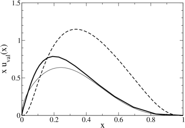
Figure 10: Longitudinal momentum distribution for a $u$ quark inside the proton. Dashed lines: our preliminary results; thick solid lines: our results after evolution to $Q^{2}$ = 1.6 (GeV/c)²; thin solid lines: CTEQ4 fit to the experimental data [10].

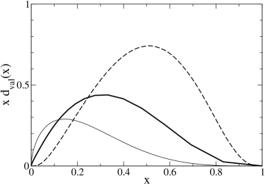
Figure 11: The same as in Fig. 10, but for a $d$ quark inside the proton.

4 CONCLUSIONS

A microscopical model for hadron em form factors in both SL and TL region has been proposed. In our model the quark-photon vertex for the process where a virtual photon materializes in a $q\bar{q}$ pair is approximated by a microscopic VMD model plus a bare term.

Both for the pion and the nucleon good results are obtained in the SL region. The Z-diagram (i.e. higher Fock state component) has been shown to be essential, in the adopted reference frame ($q^{+}\neq 0$). The possible zero in $G^{p}_{E}\mu_{p}/G^{p}_{M}$ turns out to be related to the pair-production contribution. In the TL region our calculations give a fair description of the proton and pion data, although some strength is lacking for $q^{2}=4.5$   (GeV/c)²   and   $q^{2}=8$   (GeV/c)².

The analysis of nucleon form factors allows us to get a phenomenological Ansatz for the nucleon LF wave function, which reflects the asymptotic behaviour suggested by the one-gluon-exchange dominance. This LF wave function is then used to evaluate the unpolarized transverse momentum distributions and the longitudinal momentum distributions of the quarks in the nucleon.

Our next step will be the calculation of polarized transverse and longitudinal momentum distributions.

References

• [1] S.J. Brodsky, H.C. Pauli, and S.S. Pinsky, Phys. Rep. 301, 299 (1998).
• [2] W.R.B.de Araujo, E.F. Suisso, T. Frederico, M. Beyer, H.J. Weber, Phys. Lett. B 478 (2000) 86; Nucl. Phys. A 694 (2001) 351.
• [3] S. Mandelstam, Proc. Royal Soc. A 233 (1956) 248.
• [4] J.P.B.C. de Melo, T. Frederico, E. Pace, S. Pisano and G. Salmè, Phys. Lett. B 671 (2009) 153.
• [5] J.P.B.C. de Melo, T. Frederico, E. Pace and G. Salmè, Phys. Lett. B 581 (2004) 75; Phys. Rev. D 73 (2006) 074013.
• [6] T. Frederico, H.-C. Pauli and S.-G. Zhou, Phys. Rev. D 66 (2002) 116011.
• [7] E. Pace, G. Salmè, T. Frederico, S. Pisano and J.P.B.C. de Melo, Nucl. Phys. A 782 (2007) 69c; A 790 (2007) 606c.
• [8] R. Jacob, P.J. Mulders, J. Rodriguez, Nucl. Phys. A 626 (1997) 937.
• [9] M. Anselmino, E. Efremov, A Kotzinian, B. Parsamyan, Phys. Rev. D 74 (2006) 074015.
• [10] H.L. Lai, J. Botts, J. Huston, J.G. Morfin, J.F. Owens, J.W. Qiu, W.K Tung, H. Weerts, Phys. Rev. D 51 (1995) 4763.