RM3-TH/10-02
QCD Corrections in two-Higgs-doublet extensions
of the Standard Model with Minimal Flavor Violation
G. Degrassia and P. Slavichb
a
Dipartimento di Fisica, Università di Roma Tre and INFN, Sezione di
Roma Tre
Via della Vasca Navale 84, I-00146 Rome, Italy
b LPTHE, 4, Place Jussieu, F-75252 Paris, France
We present the QCD corrections to and to the effective Hamiltonian in models with a second Higgs field that couples to the quarks respecting the criterion of Minimal Flavor Violation, thus belonging either to the or to the representation of . After the inclusion of the QCD corrections, the prediction for becomes practically insensitive to the choice of renormalization scheme for the top mass, which for the type-I and type-II models translates in a more robust lower bound on . The QCD-corrected determinations of and are used to discuss the constraints on the couplings of a (colored) charged Higgs boson to top and bottom quarks.
1 Introduction
One of the main goals of the present experimental program at the Tevatron and at the Large Hadron Collider (LHC) is the search for the Higgs boson(s) in order to elucidate the mechanism of electroweak symmetry breaking (EWSB). In the Standard Model (SM), the latter is realized in the most economical way via a single Higgs doublet. This minimal realization predicts a single neutral Higgs boson, whose mass can be constrained, from electroweak precision data and the direct search limit from LEP, to be lighter than GeV. However, at the moment, there is no direct experimental evidence for a neutral Higgs boson or any other scalar particle like, for example, a charged boson that can be present in models with a nonminimal Higgs sector.
The LHC is going to explore physics up to the TeV scale in order to search for the Higgs boson, as well as for any new phenomenon that would confirm the widespread expectation that the picture of particle physics in terms of the SM is incomplete. However, new particles with mass in the TeV range that couple to quarks at the tree level can modify the predictions for Flavor Changing Neutral Current (FCNC) processes. Thus any extension of the SM, starting from the simplest we can think of, a Two-Higgs-Doublet Model (2HDM), needs to face the problem of avoiding conflicts with the strict limits on FCNC processes.
Glashow and Weinberg addressed this issue proposing the principle of Natural Flavor Conservation (NFC) [1], which requires that the matrices of Yukawa couplings to up and down quarks for all the Higgs fields be diagonal in the basis where the quark mass matrices, , are diagonal. This implies that, with the exception of models with vectorlike quarks that mix with the ordinary ones, NFC models do not have tree-level FCNC couplings. In the 2HDM case, NFC can be realized imposing the sufficient condition that each of the quark mass matrices is obtained from a single Higgs field. This can be enforced via a symmetry that acts differently on the two Higgs doublets, leading to two possibilities usually referred to as type-I (i.e., the model in which both up and down quarks get their masses from Yukawa couplings to the same Higgs doublet) and type-II models (where up and down quarks get their masses from Yukawa couplings to different Higgs doublets).
A less-restrictive way to suppress FCNC processes, still avoiding conflict with the experimental bounds, is to consider the criterion of Minimal Flavor Violation (MFV) [2], which amounts to assuming that all the new flavor-changing transitions, including those mediated at the tree level by electrically neutral particles, are controlled by the Cabibbo-Kobayashi-Maskawa (CKM) matrix. Thus, the MFV hypothesis requires that all the flavor-violating interactions of the new particles present at the TeV scale be linked to the known structure of the Yukawa couplings.
The enforcement of the MFV hypothesis to the case of multi-Higgs models has been recently investigated by several groups [3, 4, 5]. In particular, in ref. [3] it has been shown, via group-theoretic arguments, that the MFV hypothesis can be enforced requiring that all the Higgs Yukawa-coupling matrices be composed from the pair of matrices and that are responsible for the breaking of the quark flavor symmetry. This requirement restricts the allowed representations of the Higgs fields that can couple to the quarks to either be equal to that of the SM Higgs field, i.e. , or transform as . Examples of the former case, besides the NFC type I and II models, are the aligned model of ref. [5] or the class of 2HDM presented in ref. [6]. The latter case is quite different, because the second field does not acquire a vacuum expectation value (vev) and does not mix with the SM Higgs field. Thus the scalar spectrum of this model contains a CP-even, color-singlet Higgs boson (the usual SM one) and three color-octet particles, one CP-even, one CP-odd and one electrically charged, which are split in mass proportionally to the SM-Higgs vev [3]. These colored scalar particles give rise to an interesting phenomenology for the LHC, not only because – if they are not too heavy – they can be directly produced, but also because their indirect effects can influence flavor, electroweak and Higgs physics [3, 7, 8, 9, 10].
Models with a second Higgs doublet present a new and interesting phenomenology, in particular related to the presence of a charged scalar. In the flavor sector, decays mediated by a weak charged current are the natural place where effects due to a charged Higgs boson, , can show up. In the electroweak sector the observable hadrons) shows a sensitivity to because of the specific vertex corrections introduced by the interaction of with the top and bottom quarks. Many studies (for the most recent see, e.g., refs. [11, 12, 13]) used various combinations of flavor and electroweak observables to constrain the parameter space of the type-II 2HDM, which garnered most of the attention because of its property of having the same Higgs-sector realization as the Minimal Supersymmetric Standard Model (MSSM). Other studies [14, 15, 16] explored the parameter space of 2HDMs unconstrained by a symmetry, with the second Higgs doublet still in the representation.
The theoretical accuracy of the predictions in the 2HDM with MFV is not yet at the same level as in the SM. Here we take a first step in improving this situation, by (re)considering the QCD corrections to two observables, and , which allow to set important constraints on the mass and couplings of the charged scalar. The QCD corrections can play a relevant role in reducing the error of the theoretical predictions, a well-known example of this fact being indeed the radiative decay of the meson. The present knowledge in the 2HDMs of the two observables we are considering can be summarized in this way: in the case of models with a second Higgs doublet in the representation, the complete one-loop calculation of is available [17], but (to our knowledge) no QCD corrections to the charged-scalar contributions are known. The process is instead fully known at the Next-to-Leading Order (NLO) in QCD [18, 19, 20, 21]. The case with colored scalars in the adjoint representation of is less studied. The one-loop charged-scalar contribution to was reported in ref. [7] (see also ref. [22]) while for the radiative decay of the B meson only a partial result for the Leading Order (LO) Wilson coefficients of the magnetic and chromo-magnetic operators has been presented [3].
In this paper we present the QCD corrections to the contribution to of a charged scalar in either the or the representation. Concerning , we compute the contribution to the Wilson coefficients due to a colored charged scalar in the representation. This is the missing piece to achieve NLO predictions for for all 2HDMs with MFV. Because of the specific interactions of the colored scalar with the gluons, the Wilson coefficients cannot be simply obtained by an appropriate color-factor rescaling of the known result.
The paper is organized as follows: in the next section we discuss the couplings of the charged Higgs boson in the different realizations of the 2HDM with MFV. In section 3 we present the results for the QCD-corrected contribution to due to a charged scalar, covering both cases of color-singlet and color-octet particle. We show that, after the inclusion of the QCD correction, the prediction for is practically insensitive to choice of an or on-shell (OS) renormalization scheme for the top mass. The bounds set by on the coupling are also shown. Section 4 contains the result for the NLO Wilson coefficients in the effective Hamiltonian (the explicit analytic expressions are presented in the appendix). The known results for the colorless 2HDMs are recovered, while the case of a colored charged scalar is fully new. The restrictions imposed by on the charged-scalar interaction with quarks are discussed. Finally, in section 5 we present our conclusions.
2 Minimally flavor violating 2HDMs
In a generic 2HDM it is always possible to rotate the two Higgs fields to a basis in which only one of them, which we denote as , gets a vev [23]. In this basis, we write the Yukawa interactions of the Higgs fields with the quarks as
| (1) |
where , and the Yukawa couplings are matrices in flavor space such that . The possibility of a colored second Higgs doublet is encoded in the matrices that act on the quark fields. In the usual colorless 2HDM is equal to the identity matrix in color space. On the other hand, for a colored Higgs doublet in the adjoint representation of , the matrices of the fundamental representation. The MFV condition amounts to requiring that the Yukawa coupling matrices of the second doublet, , be composed of combinations of the matrices , and transform under the quark flavor symmetry in the same way as themselves. We can decompose the matrices as
| (2) |
where in principle and are arbitrary complex coefficients. The ellipses in eq. (2) denote terms involving powers of as well as terms involving higher powers of . In the following, we will assume that the only significant deviations from proportionality between and are controlled by the Yukawa coupling of the top quark, and that terms involving higher powers of the Yukawa matrices are suppressed (e.g., because they are generated at higher loops). If we further require that there are no new sources of CP violation apart from the complex phase in the CKM matrix, the coefficients and must be real. Finally, the case corresponds to the NFC situation in which the Yukawa matrices of both Higgs doublets are aligned in flavor space.
The processes and that we will consider in sections 3 and 4 involve loops with a charged Higgs boson and a top quark. Under the assumptions implicit in eq. (2), the interaction between the quarks and is controlled by the Lagrangian
| (3) |
where is the coupling constant, are generation indices, are quark masses, is the CKM matrix. The family-dependent couplings read
| (4) |
where . It appears from eq. (4) that, when we neglect the masses of the light quarks, the effect on the charged-Higgs couplings arising from the terms in eq. (2) is limited to a shift in the couplings involving the top quark. Since those are the only couplings that enter our computations, in sections 3 and 4 we will drop the family index from without ambiguity.
The term entering the expression for in eq. (2) also induces a flavor-changing interaction with the down quarks for the neutral component of the second Higgs doublet. However, this interaction does not affect the computation of , and its contribution to is negligible with respect to the charged-Higgs contribution as long as . Other FCNC processes such as mixing would put bounds on the combination , but this will not be relevant to the discussion that follows.
In the notation of eq. (3), the type-I and type-II models are specified by equal to the identity matrix in color space, and by the real (and family-universal) coefficients
| (5) | |||||
| (6) |
where is the ratio of the vevs of the two Higgs doublets in the basis where each of the quark mass matrices is obtained from a single Higgs field.
According to our discussion, the MFV hypothesis includes two other possibilities, namely color-singlet and color-octet Higgs doublet that couple to the quarks with arbitrary coefficients111Even models with generic Yukawa matrices not satisfying the MFV hypothesis show a structure of couplings with arbitrary coefficients . To be phenomenologically viable, the dangerous FCNC effects should be sufficiently suppressed via some specific assumption like, e.g., a specific texture of the Yukawa matrices [24]. . We are going to refer to the first category (singlet) as type-III model, while the second possibility (octet) will be called type-C model.
3 Charged-Higgs contribution to including QCD corrections
We begin by discussing the radiatively corrected partial decay width of the boson in a quark-antiquark pair in a model with an additional Higgs doublet. We write it as
| (7) |
where is the color factor (), are the left-handed and right-handed couplings, written in terms of the radiative parameter and the radiatively corrected sine of the Weinberg angle as ( is the third component of the weak isospin, is the electric charge in unit )
| (8) |
while the factor contains the QCD, QED and quark-mass corrections. The latter has been computed up to in ref. [25], and at the lowest order it reads:
| (9) |
where and .
We assume that the oblique corrections due to the second doublet are negligible, as happens when the spectrum of the additional states is approximately custodially symmetric. Then the effect of the second Higgs doublet is concentrated in the vertex corrections to . Thus, defining
| (10) | |||||
| (11) |
we have . In the limit of neglecting the mass of the boson with respect to the masses of the top quark and the charged Higgs boson we find
| (12) | |||||
| (13) |
where for Higgs fields in the representation, and we omit an overall factor . In eqs. (12) and (13) , where is the quark mass at the scale and is the OS mass. The explicit expressions for the functions are
| (14) | |||||
| (15) | |||||
| (16) |
where the last term () in the function is introduced to avoid double counting due to the correction factor in eq. (7), and in the coupling we have also kept the contribution proportional to the bottom mass222Terms proportional to , relevant only for very large values of , can also arise from vertices with neutral scalars..
The one-loop terms in and agree with the results333In ref. [22] there is a misprint in the overall normalization of the couplings. of refs. [17, 22]. The two-loop terms were obtained following the lines of the analogous SM calculation that was performed by several groups, via different methods, in the early nineties [26]. The SM correction can be actually obtained by considering the SM Lagrangian in the limit of vanishing gauge coupling constants, the so-called gaugeless limit of the SM [27]. In this limit the gauge bosons play the role of external sources, and the propagating fields are those of a Yukawa theory with massless Goldstone bosons. Indeed, in the limit , the corrections in eq. (12) agree with the known SM result.
To express the corrections in terms of the OS top mass , we must expand the top mass entering the one-loop part as , with
| (17) |
For the terms proportional to and in eqs. (12) and (13), this amounts to making the substitution and replacing the function with the OS counterparts and , respectively:
| (18) |
The explicit dependence on the renormalization scale cancels out in the function :
| (19) |
whereas has a residual dependence on which is compensated for by the implicit scale dependence of the entering the one-loop parts of eqs. (12) and (13). Using the OS bottom mass would remove this residual scale dependence, but it would introduce large logarithms of the ratio in the two-loop part of the corrections.
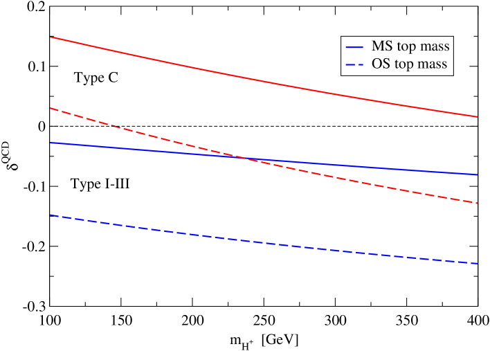
In fig. 1 we plot, as a function of , the ratio between the two-loop and one-loop contributions in the terms proportional to in eq. (12), for the two cases of color-singlet (lower set of lines) and color-octet (upper set of lines) charged Higgs boson. For each case, we show as obtained using either the central value of the physical (OS) top mass, GeV [28] (dashed lines), or the corresponding value GeV (solid lines), with the appropriate formulae for the two-loop function . It can be seen from the figure that, for models of types I–III (i.e. with color-singlet charged Higgs) the two-loop corrections are always negative, and they are substantially larger when the OS top mass is used in the one-loop part than when the mass is used. On the other hand, for the model of type C (with color-octet charged Higgs) there is an overall upward shift in the two-loop correction due to the additional function in eq. (12), with the result that the sign and relative size of the corrections in the OS and cases depend on the Higgs mass. For low values GeV, the two-loop correction approaches zero if the OS top mass is used, and it is positive and relatively large if the mass is used. Conversely, for larger values GeV the two-loop correction approaches zero if the top mass is used, and it is negative and relatively large if the OS mass is used. As a result, we will see that for 2HDMs of types I–III a reliable approximation of the two-loop result for could be obtained by using the one-loop result expressed in terms of the top mass. On the other hand, a precise determination of in the 2HDM of type C requires the inclusion of the two-loop part of the vertex correction.
From eqs. (7)–(13) we can construct the observable , which can be written as
| (20) |
where
| (21) |
Using the results of ref. [29] we find . Concerning the SM part of , to avoid relying indirectly on the measured value of , we follow ref. [12] and compute it using the values [29] and , the latter obtained from the measured value of corrected for the top-induced contributions specific to the vertex444 In ref. [12] the correcting factor 1.0063 was not introduced.. Finally the factor that includes QCD and mass corrections is obtained from ref. [25]. We find, for , .
With the values specified above for the various parameters entering eqs. (20) and (21) we find a SM prediction , nearly below the measured value [29]. Since the charged-Higgs contributions to and have the effect of further lowering , stringent bounds can be imposed on the parameters and by the requirement that the predicted value of in a 2HDM be not too far from . On the other hand, has little sensitivity on , because the terms in eqs. (12) and (13) controlled by the latter are suppressed by . Therefore, for the models of types III and C in which is a free parameter we will simplify our discussion by setting . In the 2HDMs of type I and II the parameter is related to and cannot be set independently to zero. However, due to the strong suppression of the contributions controlled by , in most of the parameter space the predictions of obtained in those two models do not differ significantly from the predictions obtained in the type-III 2HDM with . More specifically, the predictions of the type-I 2HDM, in which , are virtually indistinguishable from those of the type-III 2HDM with for all the values of consistent with the measured value of . In the 2HDM of type II, on the other hand, , and the predictions of differ from the ones obtained in the type-III 2HDM with only for very small values of .
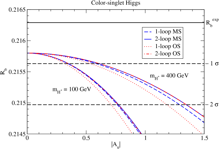
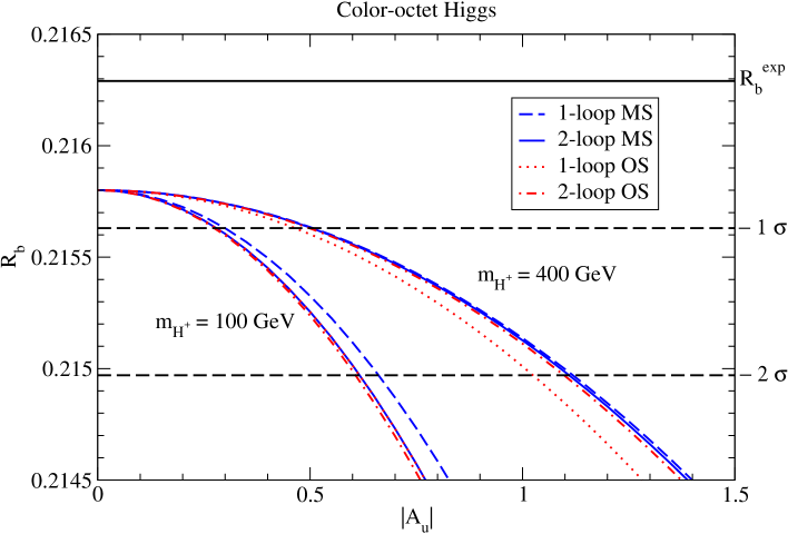
Figures 2 and 3 show our determination of in the 2HDMs of type III and C, respectively, as a function of . In each plot we show two sets of curves for the charged-Higgs mass values GeV and GeV. In each set, the dashed (solid) curve represents the one-loop (two-loop) result expressed in terms of the top mass, while the dotted (dot-dashed) curve represents the one-loop (two-loop) result expressed in terms of the physical top mass. We also show in each plot the measured value (solid horizontal line) and the values and below (dashed horizontal lines). It can be seen that, in both plots, the curves corresponding to the two-loop results (with the top mass renormalized either in the or in the OS scheme) are practically overlapped. The location of the curves corresponding to the one-loop results reflects the behavior that could already be inferred from fig. 1: in the 2HDM of type III the one-loop result computed in terms of the top mass is very close to the two-loop result, while the one-loop result computed in terms of the physical top mass can differ significantly. On the other hand, in the 2HDM of type C the quality of the one-loop approximation depends on the charged Higgs mass. At low values of , using the physical top mass in the one-loop result gives a much better approximation to the two-loop result than using the top mass, while the situation is reversed at large values of . Therefore, only the use of the two-loop results guarantees a precise determination of for all the values of .
From figures 2 and 3 it is also possible to determine the values of that are disfavored by the comparison between and the corresponding theoretical prediction. In the case of the type-III 2HDM, the two-loop curves cross the horizontal line at for GeV and at for GeV. In the case of the type-C 2HDM, they cross it at for GeV and at for GeV. We checked that the crossing points for intermediate values of can be determined by linear interpolation of the values given above.
The predictions of for the type-II 2HDM (where ) are virtually indistinguishable from those presented in figure 2 for the type-III 2HDM as soon as . The upper bounds on discussed above translate, for the type-II 2HDM, into for GeV and for GeV. On the other hand, when tends to zero the predictions of in the type-II 2HDM decrease quickly, and get two standard deviations below for , corresponding to . As we will see in the next section, the bounds on coming from the process can be much stronger than that, but they do not apply to the type-II 2HDM.
4 Charged-Higgs contribution to at the NLO
The branching ratio for is fully known at the NLO for a 2HDM of types I–III. To cover also the case of a type-C 2HDM, the only missing ingredient is the determination of the colored-scalar contribution to the Wilson coefficients. We compute it following the analogous computation for the type I–II 2HDM presented in ref. [19].
In the operator basis defined in ref. [19] we write the Wilson coefficients at the scale , where the “full” theory is matched to an effective theory with five quark flavors, as
| (22) |
where represents the SM contribution () while represents the charged-Higgs contribution. At the LO, the latter is given by
| (23) | |||||
| (24) | |||||
| (25) |
where
| (26) |
| (27) |
| (28) |
with
| (29) |
expressed in terms of the NLO top-quark running mass at the scale and of the OS charged-Higgs mass. Again, for Higgs fields in the representation.
At the NLO, the charged-Higgs contributions to the Wilson coefficients are
| (30) | |||||
| (31) | |||||
| (32) | |||||
| (33) |
The expressions for and are rather long and they are reported in the appendix. As expected, the dependence in cancels out at because the functions entering eqs. (32) and (33) satisfy the relation
| (34) |
where is the LO anomalous dimension of the top mass, while is the matrix of LO anomalous dimensions of the Wilson coefficients, whose entries can be found in eq. (8) of ref. [18].
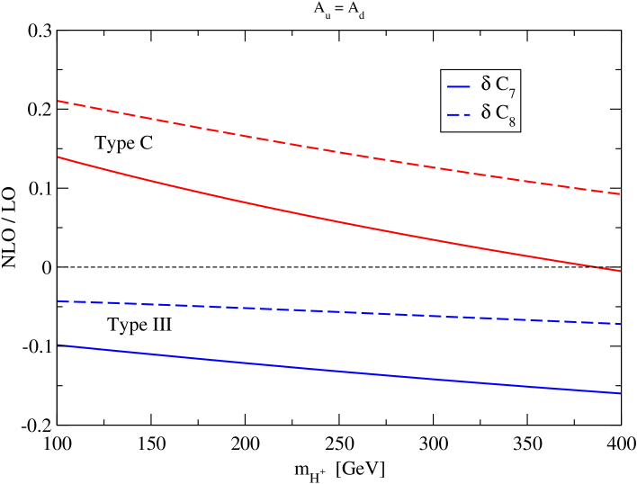
In fig. 4 we show the ratio between the NLO and LO charged-Higgs contributions to the Wilson coefficients as a function of , for both the type-C (color-octet) and type-III (color-singlet) cases, with the particular choice (in the color-singlet case this coincides with the type-I 2HDM). For the type-C 2HDM, the NLO corrections can reach up to of the LO contribution at small , and they decrease as the charged-Higgs mass increases, eventually crossing zero. In contrast, for the type-III 2HDM the two-loop corrections to the Wilson coefficients are always different from zero, and have opposite sign with respect to the LO contributions. We checked that the behavior of the NLO corrections is qualitatively similar to the one described above even when we allow to take on values different from .
The calculation of is performed using a modified version of the fortran code SusyBSG [30]. The code provides a NLO evaluation of the branching ratio in the MSSM with MFV, including the full two-loop gluino contributions to the Wilson coefficients [31]. The current public version (1.3) includes also the options of evaluating the branching ratio in the SM, in the type-II 2HDM and in the MSSM with two-loop gluino contributions computed in the effective Lagrangian approximation. We enlarged the 2HDM option to include also the type-I, type-III and type-C models, thus covering all four types of 2HDM compatible with MFV.555A public version of SusyBSG with this new feature will be released soon. The relation between the Wilson coefficients and is computed at NLO along the lines of ref. [32], but the free renormalization scales entering the NLO calculation are adjusted in such a way as to mimic the Next-to-Next-to-Leading Order (NNLO) contributions presented in ref. [33]. When the SM input parameters are set to the partially outdated values used in ref. [33], SusyBSG gives a SM prediction for of , in full agreement with the NNLO result of that paper. Very good numerical agreement is also found with the results of the partial NNLO implementation of the type-II 2HDM in ref. [33], which combines NNLO anomalous dimensions and matrix elements with NLO Wilson coefficients. We take into account a recent update [34] in the calculation of the normalization factor for the branching ratio as well as the latest central value of the top mass [28], which results in a modest enhancement of the SM prediction for to .
In the 2HDMs of types I and II, the requirement of consistency between the theoretical prediction and the measured value of allows us to set bounds on the parameters and , the latter determining both Higgs-quark couplings and . More specifically, in the type-I 2HDM the charged-Higgs contribution to the Wilson coefficients scales like , therefore it is possible to derive, for each given value of , a lower bound on (i.e., an upper bound on ) which is however much less stringent than the corresponding bound derived from . In the type-II 2HDM there is a -independent contribution to the Wilson coefficient, which allows to set an absolute lower bound on . These bounds have been extensively discussed in the literature (see, e.g., refs. [11, 12, 13]) and we will not further consider them here. In the models of type III and C, on the other hand, the parameters and are unrelated to each other. As can be seen in eqs. (24) and (25), the charged-Higgs contributions to the Wilson coefficients include two terms controlled by and , respectively. The bounds on derived in the previous section tell us that the former term cannot be too large, while the latter can be significant for large values of . Furthermore, its effect on the branching ratio depends on the relative sign between and .
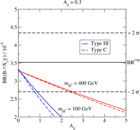
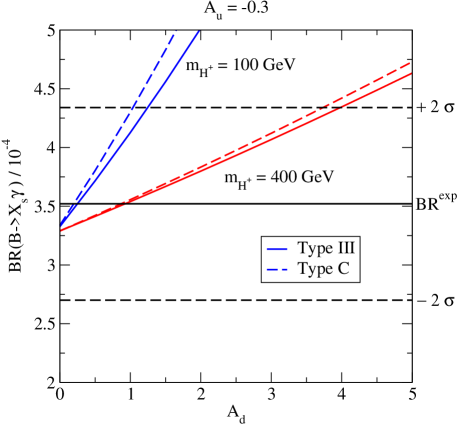
In fig. 5 we show as a function of , for both the type-III (solid lines) and type-C (dashed lines) 2HDM, and for the representative choices (the latter are allowed by , as can be seen in figs. 2 and 3). The left panel displays the case of same sign between and , while the right panel shows the case of opposite sign. Each plot contains two sets of curves corresponding to 100 GeV and GeV, respectively. The horizontal dashed lines mark the 95% C.L. band around the experimental value [35]. The band also includes, added in quadrature, the theoretical error on the 2HDM prediction (we conservatively estimate this error as 10% of the SM prediction for the branching ratio). From fig. 5 it is clear that, unless is extremely small, the process sets stringent limits on . Focusing on the case of color-singlet Higgs we see that, for , the values of that allow for a branching ratio inside the 95% C.L. band are for GeV and for GeV; for the bounds are a little less stringent, i.e. for GeV and for GeV. From the figure it is also apparent that the bound on for a fixed value of is almost independent of the colored or colorless nature of the charged Higgs, with the colored case showing only slightly stronger bounds. However, as seen in the previous section, the bounds on derived from are more dependent on the nature of the Higgs, so that the allowed regions for the coefficient are in fact different for the color-singlet and color-octet charged Higgs.
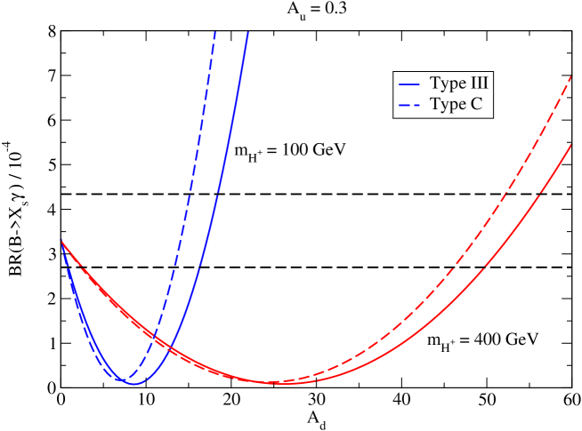
The case of same sign between and has the peculiarity that, as shown in fig. 6, there are actually two ranges of values of that fit inside the allowed band for . This is related to the fact that, in this case, the sign of the charged-Higgs contribution to the Wilson coefficient of the magnetic dipole operator, , is opposite to the sign of the SM contribution, . Since is roughly proportional to , as increases the branching ratio goes to zero when , and it goes back inside the -allowed band when . Thus, the two ranges of possible values of differ by the sign of the amplitude , basically the sign of the Wilson coefficient . Although allows both ranges of values for , there are other observables that are sensitive to the sign of , thus selecting one of the two options. Among them, we cite [36] and the isospin-breaking asymmetry that can be constructed from the exclusive neutral and charged decay modes [37, 16]. Although, for both observables, neither the experimental result nor the theoretical prediction is at the same level of accuracy as for , these observables still give a compelling indication that the sign of is that of the SM contribution, thus eliminating the large- option.
5 Conclusions
Minimal flavor violation is a very popular criterion that is used to suppress FCNC effects in models with new particles at the TeV scale. The enforcement of the MFV criterion to the simplest extension of the SM, i.e. a model with a second Higgs doublet, allows the possibility of color-singlet or color-octet Higgs field. For both cases we have considered the two-loop QCD corrections to the charged Higgs boson contribution to . We found that for all four types of 2HDM with MFV, after the inclusion of the two-loop QCD corrections, the prediction for this observable is practically insensitive to the the choice of renormalization scheme for the top mass entering the one-loop part of the calculation. Thus, the upper bound on the coupling derived from is improved, which for the type-I and type-II models translates in a more robust lower bound on . We have also computed the contributions to the Wilson coefficients relevant to the process for the color-octet case. This was the last missing ingredient to obtain a determination of at the NLO level for all 2HDM with MFV. After the inclusion of the NLO corrections it is found that, in the region allowed by the present experimental results, the transition is fairly insensitive to the colored or colorless nature of the charged Higgs. Furthermore, in type-III and C models, the bounds on the parameter that can be obtained from and other observables rule out the large- region, where effects proportional to the bottom mass could become important.
Acknowledgments
We thank H. Haber for communications concerning ref. [22], and P. Gambino for useful discussions. One of us (G.D.) also thanks M. Nebot for his contribution in the early stage of this project. This work was supported in part by an EU Marie-Curie Research Training Network under contract MRTN-CT-2006-035505 (HEPTOOLS) and by ANR under contract BLAN07-2_194882.
Appendix: Analytical expressions for the NLO Wilson coefficients
In this appendix we report the analytic expressions for the functions and entering . We find
| (A1) | |||||
| (A2) | |||||
| (A3) | |||||
| (A4) | |||||
| (A5) | |||||
The results for type I-III models are recovered setting and , while the result for the case of a colored charged scalar in the adjoint of is obtained with and .
Note added:
after the publication of our paper, we became aware of ref. [38], which contains two-loop formulae for the Wilson coefficients of the operators relevant to in a generic model with a heavy fermion and a heavy scalar. While ref. [38] does not specifically discuss the case of the type-C 2HDM, the results presented in our appendix can be reproduced with appropriate substitutions in the results of ref. [38], taking into account the different renormalization conditions on the charged-Higgs mass. We thank Christoph Bobeth for performing this useful comparison.
References
- [1] S. L. Glashow and S. Weinberg, Phys. Rev. D 15 (1977) 1958.
-
[2]
R. S. Chivukula and H. Georgi,
Phys. Lett. B 188 (1987) 99;
G. D’Ambrosio, G. F. Giudice, G. Isidori and A. Strumia, Nucl. Phys. B 645 (2002) 155 [arXiv:hep-ph/0207036]. - [3] A. V. Manohar and M. B. Wise, Phys. Rev. D 74 (2006) 035009 [arXiv:hep-ph/0606172].
- [4] F. J. Botella, G. C. Branco and M. N. Rebelo, arXiv:0911.1753 [hep-ph].
- [5] A. Pich and P. Tuzon, Phys. Rev. D 80 (2009) 091702 [arXiv:0908.1554 [hep-ph]].
- [6] G. C. Branco, W. Grimus and L. Lavoura, Phys. Lett. B 380 (1996) 119 [arXiv:hep-ph/9601383].
- [7] M. I. Gresham and M. B. Wise, Phys. Rev. D 76 (2007) 075003 [arXiv:0706.0909 [hep-ph]].
- [8] A. Idilbi, C. Kim and T. Mehen, Phys. Rev. D 79 (2009) 114016 [arXiv:0903.3668 [hep-ph]].
- [9] R. Bonciani, G. Degrassi and A. Vicini, JHEP 0711 (2007) 095 [arXiv:0709.4227 [hep-ph]].
- [10] C. P. Burgess, M. Trott and S. Zuberi, JHEP 0909 (2009) 082 [arXiv:0907.2696 [hep-ph]].
- [11] H. Flacher, M. Goebel, J. Haller, A. Hocker, K. Moenig and J. Stelzer, Eur. Phys. J. C 60 (2009) 543 [arXiv:0811.0009 [hep-ph]].
- [12] O. Deschamps, S. Descotes-Genon, S. Monteil, V. Niess, S. T’Jampens and V. Tisserand, arXiv:0907.5135 [hep-ph].
- [13] M. Bona et al. [UTfit Collaboration], Phys. Lett. B 687 (2010) 61 [arXiv:0908.3470 [hep-ph]].
- [14] J. P. Idarraga, R. Martinez, J. A. Rodriguez and N. Poveda, Braz. J. Phys. 38 (2008) 531.
- [15] J. L. Diaz-Cruz, J. Hernandez–Sanchez, S. Moretti, R. Noriega-Papaqui and A. Rosado, Phys. Rev. D 79 (2009) 095025 [arXiv:0902.4490 [hep-ph]].
- [16] F. Mahmoudi and O. Stal, Phys. Rev. D 81 (2010) 035016 [arXiv:0907.1791 [hep-ph]].
- [17] A. Denner, R. J. Guth, W. Hollik and J. H. Kuhn, Z. Phys. C 51 (1991) 695.
- [18] K. G. Chetyrkin, M. Misiak and M. Munz, Phys. Lett. B 400 (1997) 206 [Erratum-ibid. B 425 (1998) 414] [arXiv:hep-ph/9612313], and references therein.
- [19] M. Ciuchini, G. Degrassi, P. Gambino and G. F. Giudice, Nucl. Phys. B 527 (1998) 21 [hep-ph/9710335].
- [20] P. Ciafaloni, A. Romanino and A. Strumia, Nucl. Phys. B 524 (1998) 361 [arXiv:hep-ph/9710312].
- [21] F. Borzumati and C. Greub, Phys. Rev. D 58 (1998) 074004 [arXiv:hep-ph/9802391], Phys. Rev. D 59 (1999) 057501. [arXiv:hep-ph/9809438].
- [22] H. E. Haber and H. E. Logan, Phys. Rev. D 62 (2000) 015011 [arXiv:hep-ph/9909335].
- [23] S. Davidson and H. E. Haber, Phys. Rev. D 72 (2005) 035004 [Erratum-ibid. D 72 (2005) 099902] [arXiv:hep-ph/0504050].
- [24] T. P. Cheng and M. Sher, Phys. Rev. D 35 (1987) 3484.
- [25] K. G. Chetyrkin, J. H. Kuhn and A. Kwiatkowski, arXiv:hep-ph/9503396.
-
[26]
J. Fleischer, O. V. Tarasov, F. Jegerlehner and P. Raczka,
Phys. Lett. B 293 (1992) 437;
G. Buchalla and A. J. Buras, Nucl. Phys. B 398 (1993) 285;
G. Degrassi, Nucl. Phys. B 407 (1993) 271 [arXiv:hep-ph/9302288]. - [27] R. Barbieri, M. Beccaria, P. Ciafaloni, G. Curci and A. Vicere, Phys. Lett. B 288, 95 (1992) [Erratum-ibid. B 312, 511 (1993)] [arXiv:hep-ph/9205238].
- [28] [Tevatron Electroweak Working Group and CDF Collaboration and D0 Collab], arXiv:0903.2503 [hep-ex].
- [29] [ALEPH Collaboration and DELPHI Collaboration and L3 Collaboration and ], Phys. Rept. 427 (2006) 257 [arXiv:hep-ex/0509008].
- [30] G. Degrassi, P. Gambino and P. Slavich, Comput. Phys. Commun. 179 (2008) 759 [arXiv:0712.3265 [hep-ph]].
- [31] G. Degrassi, P. Gambino and P. Slavich, Phys. Lett. B 635 (2006) 335 [arXiv:hep-ph/0601135].
- [32] P. Gambino and M. Misiak, Nucl. Phys. B 611 (2001) 338 [arXiv:hep-ph/0104034].
- [33] M. Misiak et al., Phys. Rev. Lett. 98 (2007) 022002 [arXiv:hep-ph/0609232].
- [34] P. Gambino and P. Giordano, Phys. Lett. B 669 (2008) 69 [arXiv:0805.0271 [hep-ph]].
- [35] E. Barberio et al. [Heavy Flavor Averaging Group], arXiv:0808.1297 [hep-ex].
- [36] P. Gambino, U. Haisch and M. Misiak, Phys. Rev. Lett. 94 (2005) 061803 [arXiv:hep-ph/0410155].
- [37] A. L. Kagan and M. Neubert, Phys. Lett. B 539 (2002) 227 [arXiv:hep-ph/0110078].
- [38] C. Bobeth, M. Misiak and J. Urban, Nucl. Phys. B 567 (2000) 153 [arXiv:hep-ph/9904413].