Discovery of Convoys in Trajectory Databases

Abstract

As mobile devices with positioning capabilities continue to proliferate, data management for so-called trajectory databases that capture the historical movements of populations of moving objects becomes important. This paper considers the querying of such databases for convoys, a convoy being a group of objects that have traveled together for some time.

More specifically, this paper formalizes the concept of a convoy query using density-based notions, in order to capture groups of arbitrary extents and shapes. Convoy discovery is relevant for real-life applications in throughput planning of trucks and carpooling of vehicles. Although there has been extensive research on trajectories in the literature, none of this can be applied to retrieve correctly exact convoy result sets. Motivated by this, we develop three efficient algorithms for convoy discovery that adopt the well-known filter-refinement framework. In the filter step, we apply line-simplification techniques on the trajectories and establish distance bounds between the simplified trajectories. This permits efficient convoy discovery over the simplified trajectories without missing any actual convoys. In the refinement step, the candidate convoys are further processed to obtain the actual convoys. Our comprehensive empirical study offers insight into the properties of the paper’s proposals and demonstrates that the proposals are effective and efficient on real-world trajectory data.

1 Introduction

Although the mobile Internet is still in its infancy, very large volumes of position data from moving objects are already being accumulated. For example, Inrix, Inc. based in Kirkland, WA receive real-time GPS probe data from more than 650,000 commercial fleet, delivery vehicles, and taxis [1]. As the mobile Internet continues to proliferate and as congestion becomes increasingly widespread across the globe, the volumes of position data being accumulated are likely to soar. Such data may be used for many purposes, including travel-time prediction, re-routing, and the identification of ride-sharing opportunities. This paper addresses one particular challenge to do with the extraction of meaningful and useful information from such position data in an efficient manner.

The movement of an object is given by a continuous curve in the $(\mbox{space},\mbox{time})$ domain, termed a trajectory. The past trajectory of an object is typically approximated based on a collection of time-stamped positions, e.g., obtained from a GPS device. As an example, Figure 1(a) depicts the trajectories of four objects $o_{1}$, $o_{2}$, $o_{3}$, and $o_{4}$ in $(x,y,t)$ space.

Given a collection of trajectories, it is of interest to discover groups of objects that travel together for more than some minimum duration of time. A number of applications may be envisioned. The identification of delivery trucks with coherent trajectory patterns may be used for throughput planning. The discovery of common routes among commuters may be used for the scheduling of collective transport. The identification of cars that follow the same routes at the same time may be used for the organization of carpooling, which may reduce congestion, pollution, and CO₂ emissions.

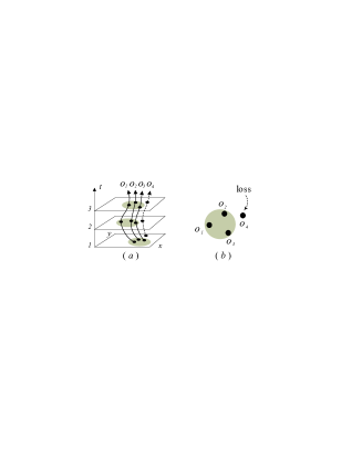
Figure 1: Lossy-flock Problem

The discovery of so-called flocks [5, 13, 14] has received some attention. A flock is a group of objects that move together within a disc of some user-specified size. On the one hand, the chosen disk size has a substantial effect on the results of the discovery process. On the other hand, the selection of a proper disc size turns out to be difficult, as situations can occur where objects that intuitively belong together or do not belong together are not quite within any disk of the given size or are within such a disk. And for some data sets, no single appropriate disc size may exist that works well for all parts of the $(\mbox{space},\mbox{time})$ domain. In Figure 1(a), all objects travel together in a natural group. However, as shown in Figure 1(b), object $o_{4}$ does not enter the disc and is not discovered as a member of the flock. A key reason why this lossy-flock problem occurs is that what constitutes a flock is very sensitive to the user-specified disc size, which is independent of the data distribution. In addition, the use of a circular shape may not always be appropriate. For example, suppose that two different groups of cars move across a river and each group has a long linear form along roads. A sufficient disc size for capturing one group may also capture the other group as one flock. Ideally, no particular shape should be fixed apriori.

To avoid rigid restrictions on the sizes and shapes of the trajectory patterns to be discovered, we propose the concept of convoy that is able to capture generic trajectory pattern of any shape and any extent. This concept employs the notion of density connection [12], which enables the formulation of arbitrary shapes of groups. Given a set of trajectories $O$, an integer $m$, a distance value $e$, and a lifetime $k$, a convoy query retrieves all groups of objects, i.e., convoys, each of which has at least $m$ objects so that these objects are so-called density–connected with respect to distance $e$ during $k$ consecutive time points. Intuitively, two objects in a group are density–connected if a sequence of objects exists that connects the two objects and the distance between consecutive objects does not exceed $e$. (The formal definition is given in Section 3.) Each group of objects in the result of a convoy query is associated with the time intervals during which the objects in the group traveled together.

The efficient discovery of convoys in a large trajectory database is a challenging problem. Convoy queries compute sets of objects and are more expensive to process than spatio-temporal joins [7], which compute pairs of objects. Past studies on the retrieval of similar trajectories generally use distance functions that consider the distances between pairs of trajectories across all of time [10, 15, 25]. In contrast, we consider distances during relatively short durations of time. Other relevant work concerns the clustering of moving objects [17, 19, 21]. In these works, a moving cluster exists if a shared set of objects exists across adjacent time, but objects may join and leave a cluster during the cluster’s lifetime. Hence, moving clusters carry different semantics and do not necessarily qualify as convoys.

Jeung et. al. first proposed the convoy query and outlined preliminary techniques for convoy discovery [4]. In this paper, we extend the work, which develops more advanced algorithms and analyzes each discovery method in real world settings. Specifically, we introduce four effective and efficient algorithms for answering the convoy query. The first method adopts the solution for moving cluster discovery to our convoy problem. The second method, called CuTS (Convoy Discovery using Trajectory Simplification), employs the filter-refinement framework — a set of candidate convoys are retrieved in the filter step, and then they are further processed in the refinement step to produce the actual convoys. In the filter step, we apply line simplification techniques [11] on the trajectories to reduce their sizes; hence, it becomes very efficient to search for convoys over simplified trajectories. We establish distance bounds between simplified trajectories, in order to ensure that no actual convoy is missing from the candidate convoy set. The third method (CuTS+) accelerates the process of trajectory simplification of CuTS to increase the efficiency of the filter step even further. The last method, named CuTS*, is an advanced version of CuTS that enhances the effectiveness of the filter step by introducing tighter distance bounds for simplified trajectories.

The main novelties of this paper are summarized as follows:

• Our filter step operates on trajectories processed by line simplification techniques; this is different from most related works that employ spatial approximation (e.g., bounding boxes) in the filter step. The rationale is that conventional methods using bounding boxes introduce substantial empty space, rendering them undesirable for the processing of trajectory data.

• To guarantee correct convoy discovery, we establish distance bounds for range search over simplified trajectories. In contrast, the distance bounds studied elsewhere [8] are applicable only to specific query types, not to the convoy problem.

• We study various trajectory simplification techniques in conjunction with different query processing mechanisms. In addition, we show how to tighten the distance bounds.

• We present comprehensive experimental results using several real trajectory data sets, and we explain the advantages and disadvantages of each proposed method.

The remainder of this paper is organized as follows: In Section 2, we discuss previous methods related to the convoy query. We formulate the focal problem of this paper in Section 3. A modified method of moving cluster for the convoy discovery is shown in Section 4. We propose more efficient methods based on trajectory simplification in Sections 5 and 6. Section 7 reports the results of experimental performance comparisons, followed by conclusions in Section 8.

2 Related Work

We first review existing work on trajectory clustering and, then cover trajectory simplification, which is an important aspect of our techniques for convoy discovery. We end by considering spatio-temporal joins and distance measures for trajectories.

2.1 Clustering over Trajectories

Given a set of points, the goal of spatial clustering is to form clusters (i.e., groups) such that (i) points within the same cluster are close to each other, and (ii) points from different clusters are far apart. In the context of trajectories, the locations of trajectories can be clustered at chosen time points. Consider the trajectories in Figure 2(a). We first obtain a cluster $c_{1}$ at time $t=1$, then a cluster $c_{2}$ at $t=2$, and eventually a cluster $c_{3}$ at $t=3$.

Kalnis et al. propose the notion of a moving cluster [19], which is a sequence of spatial clusters appearing during consecutive time points, such that the portion of common objects in any two consecutive clusters is not below a given threshold parameter $\theta$, i.e., $\frac{|c_{t}\cap c_{t+1}|}{|c_{t}\cup c_{t+1}|}\geq\theta$, where $c_{t}$ denotes a cluster at time $t$. There is a significant difference between a convoy and a moving cluster. For instance, in Figure 2(a), $o_{2},o_{3}$, and $o_{4}$ form a convoy with 3 objects during 3 consecutive time points. On the other hand, if we set $\theta=1$ (i.e., require 100% overlapping clusters), the overlap between $c_{1}$ and $c_{2}$ is only $\frac{3}{4}$, and the above objects will not be discovered as a moving cluster. Next, in Figure 2(b), if we set $\theta=\frac{1}{2}$ then $c_{1}$, $c_{2}$, and $c_{3}$ become a moving cluster. However, this is not a convoy.

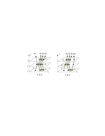
Figure 2: Convoys Versus Moving Clusters

Spiliopoulou et al. [24] study transitions in moving clusters (e.g., disappearance and splitting) between consecutive time points. As transitions are based on the consideration of common objects at consecutive time points, their techniques do not support convoy discovery either. Next, Li et al. [21] study the notion of moving micro cluster, which is a group of objects that are not only close to one another at the current time, but are also expected to move together in the near future. Recently, Lee et al. [20] have proposed to partition trajectories into line segments and build groups of close segments. This proposal does not consider the temporal aspects of the trajectories. As a result, some objects can belong to the same group even though they have never traveled close together (at the same time). Most recently, Jensen et al. [17] have proposed techniques for maintaining clusters of moving objects. They consider the clustering of the current and near-future positions, while we consider past trajectories.

As mentioned earlier, several slightly different notions of a flock [13, 14] relate to that of a convoy. The notion most relevant to our study defines a flock as a group of at least $m$ objects staying together within a circular region of radius $e$ during a specified time interval [5, 13]. Al-Naymat et al. [5] apply random projection to reduce the dimensionality of the data and thus obtain better performance. Gudmundsson et al. [13] propose approximation techniques and exploit an index to accelerate the computation of flock. It is also shown that the discovery of the longest-duration flock is an NP-hard problem. It is worth noticing that these studies exhibit the lossy-flock problem identified in Section 1.

2.2 Trajectory Simplification

A trajectory is often represented as a polyline, which is a sequence of connected line segments. Line simplification techniques have been proposed to simplify polylines according to some user-specified resolution [11, 16].

The Douglas-Peucker algorithm (DP) [11] is a well-known and efficient method among the line simplification techniques. Given a polyline specified by a sequence of $T$ points $\langle p_{1},p_{2},\cdots,p_{T}\rangle$ and a distance threshold $\delta$, the goal is to derive a new polyline with fewer points while deviating from the original polyline by at most $\delta$. The DP algorithm initially constructs the line segment $\overline{p_{1}p_{T}}$. It then identifies the point $p_{i}$ farthest from the line. If this point’s (perpendicular) distance to the line is within $\delta$ then DP returns $\overline{p_{1}p_{T}}$ and terminates. Otherwise, the line is decomposed at $p_{i}$, and DP is applied recursively to the sub-polylines $\langle p_{1},p_{2},\cdots,p_{i}\rangle$ and $\langle p_{i},\cdots,p_{T}\rangle$. As the worst-case time complexity of this algorithm is $O(T^{2})$, Hershberger et al. [16] show a faster version of this method with time complexity of $O(T\cdot\log T)$. However, it is assumed that an object’s trajectory cannot intersect itself, which is not a valid assumption for the data we consider.

The DP technique deals with line simplification only in the spatial domain, ignoring the time domain of the trajectories. Consider the example in Figure 3(a). Since the distance from $p_{2}$ to $\overline{p_{1}p_{3}}$ is within $\delta$, the DP algorithm omits $p_{2}$ and simply returns $\overline{p_{1}p_{3}}$. Similarly, $q_{2}$ is also omitted and the polygon is simplified to $\overline{q_{1}q_{3}}$.

In contrast, Meratnia et al. [23] take into account the temporal aspects in line simplification. Figure 3(b) exemplifies the working procedure of their algorithm (say, DP*). First, DP* derives the point $p^{\prime}_{2}$ on the line $\overline{p_{1}p_{3}}$ by calculating the ratio of $p_{2}$’s time between $t$=1 of $p_{1}$ and $t$=3 of $p_{3}$. Then, it measures the distance $D(p_{2},p^{\prime}_{2})$ between $p_{2}$ and $p^{\prime}_{2}$, instead of the perpendicular distance from $p_{2}$ to $\overline{p_{1}p_{3}}$. Since $D(p_{2},p^{\prime}_{2})>\delta$, $p_{2}$ is still kept after the simplification, while it was removed by using DP in Figure 3(a).

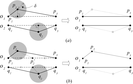
Figure 3: Comparison of Different Trajectory Simplifications

2.3 Distance Measures and Joins

A basic way of measuring the distance between two trajectories used in the literature is to compute the sum of their Euclidean distances over time points. Such a distance measure may not be able to capture the inherent distance between trajectories because it does not take into account particular features of trajectories (e.g., noise, time distortion). Thus, it is important to devise a distance function that “understands” the characteristics of trajectories.

A well-known approach is Dynamic Time Warping (DTW) [25], which applies dynamic programming for aligning two trajectories in such a way that their overall distance is minimized. More recent proposals for trajectory distance functions include Longest Common Subsequence (LCSS) [15], Edit Distance on Real Sequence (EDR) [10], and Edit distance with Real Penalty (ERP) [9]. Lee et al. [20] point out that the above distance measures capture the global similarity between two trajectories, but not their local similarity during a short time interval. Thus, these measures cannot be applied in a simple manner for convoy discovery.

Given two data sets $P_{1}$ and $P_{2}$, spatio-temporal joins find pairs of elements from the two sets that satisfy predicates with both spatial and temporal attributes [18]. The close-pair join reports all object pairs ($o_{1}$, $o_{2}$) from $P_{1}\times P_{2}$ with distance $D_{\tau}(o_{1},o_{2})\leq e$ within a time interval $\tau$ being bounded by a user-specified distance $e$. Plane-sweep techniques [6, 26] have been proposed for evaluating spatio-temporal joins. Like the close-pair join, the trajectory join [7] aims at retrieving all pairs of similar trajectories between two datasets. Bakalov et al. [7] represent trajectories as sequences of symbols and apply sliding window techniques to measure the symbolic distance between possible pairs. These studies consider pairs of objects, whereas we consider sets of objects.

3 Problem Definition

This section formalizes the convoy problem. We start with the definitions of distances for points, line segments, and bounding boxes :

Definition 1

(Distance Functions)

• Given two points $p_{u}$ and $p_{v}$, $D(p_{u},p_{v})$ is defined as the Euclidean distance between $p_{u}$ and $p_{v}$.

• Given a point $p$ and a line segment $l$, $D_{PL}(p,l)$ is defined as the shortest (Euclidean) distance between $p$ and any point on $l$.

• Given two line segments $l_{u}$ and $l_{v}$, $D_{LL}(l_{u},l_{v})$ is defined as the shortest (Euclidean) distance between any two points on $l_{u}$ and $l_{v}$, respectively.

• With $\mathcal{B}_{u}$ and $\mathcal{B}_{v}$ being boxes then $D_{min}(\mathcal{B}_{u},\mathcal{B}_{v})$ is defined as the minimum distance between any pair of points belonging to each of the two boxes.

The boxes introduced in the definition will be used for the bounding of line segments. Next, the time domain is defined as the ordered set $\{t_{1},t_{2},\cdots,t_{T}\}$, where $t_{j}$ is a time point and $T$ is the total number of time points.

In our problem setting, we consider a practical trajectory database model. We assume each trajectory may have a different length from others and may also appear or disappear at any time in $T$. In addition, each location of a trajectory can be sampled either regularly (e.g., every second) or irregularly (i.e, some missing time points from $T$ may exist between two consecutive time points of the trajectory).

The trajectory of an object $o$ is represented by a polyline that is given as a sequence of timestamped locations $o=\langle p_{a},p_{a+1},\cdots,p_{b}\rangle$, where $p_{j}=(x_{j},y_{j},t_{j})$ indicates the location of $o$ at time $t_{j}$, with $t_{a}$ being the start time and $t_{b}$ being the end time. The time interval of $o$ is $o.\tau=[t_{a},t_{b}]$. A shorthand notation is to use $o(t_{j})$ for referring to the location of $o$ at time $t_{j}$ (i.e., location $p_{j}$).

Figure 4 illustrates the polylines representing the trajectories of three objects $o_{1},o_{2}$, and $o_{3}$, during the time interval from $t_{1}$ to $t_{4}$.

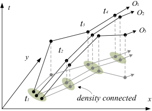
Figure 4: An Example of a Convoy

As a precursor to defining the convoy query, we need to understand the notion of density connection [12]. Given a distance threshold $e$ and a set of points $S$, the $e$-neighborhood of a point $p$ is given as $\mathit{NH}_{e}(p)=\{q\in S\;|\;D(p,q)\leq e$}. Then, given a distance threshold $e$ and an integer $m$, a point $p$ is directly density–reachable from a point $q$ if $p\in\mathit{NH}_{e}(q)$ and $|\mathit{NH}_{e}(q)|\geq m$. A point $p$ is said to be density–reachable from a point $q$ with respect to $e$ and $m$ if there exists a chain of points $p_{1}$, $p_{2}$, …, $p_{n}$ in set $S$ such that $p_{1}=q$, $p_{n}=p$, and $p_{i+1}$ is directly density–reachable from $p_{i}$.

Definition 2

(Density–Connected) Given a set of points $S$, a point $p\in S$ is density–connected to a point $q\in S$ with respect to $e$ and $m$ if there exists a point $x\in S$ such that both $p$ and $q$ are density–reachable from $x$.

The definition of density–connection permits us to capture a group of “connected” points with arbitrary shape and extent, and thus to overcome the the lossy-flock problem shown in Figure 1. By considering density–connected objects for consecutive time points, we define the convoy query as follows:

Definition 3

(Convoy Query) Given a set of trajectories of $N$ objects, a distance threshold $e$, an integer $m$, and an integer lifetime $k$, the convoy query returns all possible groups of objects, so that each group consists of a (maximal) set of density-connected objects with respect to $e$ and $m$ during at least $k$ consecutive time points.

Consider the convoy query with the parameters $m=2$ and $k=3$ issued over the trajectories in Figure 4. $\langle{o_{2},o_{3}},[t_{1},t_{3}]\rangle$ is the result, meaning that $o_{2}$ and $o_{3}$ belong to the same convoy during consecutive time points from $t_{1}$ to $t_{3}$.

Table 1 offers the notations introduced in this section and to be used throughout the paper.

Symbol	Meaning
$p$	Point/location (in the spatial domain)
$t$	Time point
$o_{i}$	Original trajectory of an object
$o_{i}(t)$	Location of $o_{i}$ at time $t$
$o^{\prime}_{i}$	Simplified trajectory (of $o_{i}$)
$l^{\prime}_{i}$	Line segment of $o^{\prime}_{i}$
$o^{\prime}_{i}.\tau$	Time interval of $o^{\prime}_{i}$
$l^{\prime}_{i}.\tau$	Time interval of $l^{\prime}_{i}$
$D(p_{u},p_{v})$	Euclidean distance between points
$D_{PL}(p,l)$	The shortest distance from point to line segment
$D_{LL}(l_{u},l_{v})$	The shortest distance between line segments
$\mathcal{B}(l)$	The minimum bounding box of $l$
$D_{min}(\mathcal{B}_{u},\mathcal{B}_{v})$	The minimum distance between two boxes

Table 1: Summary of Notation

4 Coherent Moving Cluster (CMC)

A simple technique for computing a convoy is to first perform (density–connected) clustering on the objects at each time and then to extract their common objects in an attempt to form convoys. This approach is similar to the methods for discovering moving clusters [19]. However, those are unable to discover the exact convoy results, as explained next:

• Let $c_{t}$ and $c_{t+1}$ be (snapshot) clusters at times $t$ and $t+1$. These clusters belong to the same moving cluster if they share at least the fraction $\theta$ objects ($|c_{t}\cap c_{t+1}|/|c_{t}\cup c_{t+1}|\geq\theta$), where $\theta$ is a user-specified threshold value between 0 and 1. The problem of applying moving cluster methods for convoy discovery is that no absolute $\theta$ value exists that can be used to compute the exact convoy results—either false hits may be found, or actual convoys may remain undiscovered, as explained in Section 2.1.

• A moving cluster can be formed as long as two snapshot clusters have at least $\theta$ overlap, even for only two consecutive time. The lifetime ($k$) constraint does not apply to moving clusters, but is essential for a convoy.

• As pointed in the previous section, a trajectory may have some missing time points due to irregular location sampling (e.g., $o_{3}$ at $t=2$ in Figure  5(a)). In this case, we cannot measure the density–connection for all objects involved over those missing times.

In order to solve the above problems for convoy discovery, we extend the moving cluster method into our Coherent Moving Cluster algorithm (CMC). First, we generate virtual locations for the missing time points. If any trajectory has a location at time $t_{i}$, but another does not during its time interval, we apply linear interpolation to create the virtual points at $t_{i}$. Second, to accommodate the lifetime ($k$) constraint, we require each candidate convoy to have (at least) $k$ clusters $c_{t},c_{t+1},\cdots,c_{t+k-1}$ during consecutive time points. Third, we test the condition $|c_{t}\cap c_{t+1}\cap\cdots\cap c_{t+k-1}|\geq m$, to determine whether sufficiently many common objects are shared. If all conditions are satisfied, the candidate is reported as an actual convoy.

We proceed to illustrate algorithm CMC using Figure 5, with the parameters $m=2$ and $k=3$. Let $c_{t}^{i}$ be the $i$-th snapshot cluster at time $t$. Clusters at time $t$ are obtained by applying a snapshot density clustering algorithm (e.g., DBSCAN [12]) on the objects’ locations at time $t$.

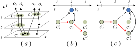
Figure 5: Query Processing of CMC, $m=2$

Table 2 illustrates the execution steps of the algorithm. At time $t_{1}$, we obtain a cluster $c_{1}^{1}$ (with objects $o_{1}$, $o_{2}$, and $o_{3}$) and consider it a convoy candidate $v_{1}$. At time $t_{2}$, we retrieve a cluster $c_{2}^{1}$, which is then compared with $v_{1}$. Since $c_{2}^{1}$ and $v_{1}$ have $m=2$ common objects, we compute their intersection and update candidate $v_{1}$. At time $t_{3}$, we discover two clusters $c_{3}^{1}$ and $c_{3}^{2}$. Since $c_{3}^{1}$ shares no objects with $v_{1}$, we consider $c_{3}^{1}$ as another convoy candidate $v_{2}$. As $c_{3}^{2}$ shares $m=2$ common objects with $v_{1}$, we update $v_{1}$ to be its intersection with $c_{3}^{2}$. Eventually, $v_{1}$ is reported as a convoy because it contains $m=2$ common objects from clusters during $k=3$ consecutive time points.

Timestamp	Clusters	Candidate set $V$
$t_{1}$	$c_{1}^{1}$	$v_{1}=c_{1}^{1}$
$t_{2}$	$c_{2}^{1}$	$v_{1}=c_{1}^{1}\cap c_{2}^{1}$
$t_{3}$	$c_{3}^{1}$, $c_{3}^{2}$	$v_{1}=c_{1}^{1}\cap c_{2}^{1}\cap c_{3}^{2}$, $v_{2}=c_{3}^{1}$

Table 2: Execution Steps of CMC

Algorithm 1 presents the pseudocode for the CMC algorithm. The algorithm takes as inputs a set of object trajectories $O$ and convoy query parameters $m$, $k$, and $e$.

We use $V$ to represent the set of convoy candidates. We then perform processing for each time point (in ascending order). The set $V_{next}$ introduced in Line 3 is used to store candidates produced at the current time $t$. Then, we consider only objects $o\in O$ whose time intervals cover time $t$, i.e., $t\in o.\tau$. Their locations $o(t)$ are inserted into the set $O_{t}$. If any object $o\in O_{t}$ has a missing location at $t$, a virtual point is computed and then inserted.

Next, we apply DBSCAN on $O_{t}$ to obtain a set $C$ of clusters (Line 7). The clusters in $C$ are compared to existing candidates in $V$. If they share at least $m$ common objects (Line 11), the current objects of the candidate $v$ are replaced by the common objects between $c$ and $v$ and are then inserted into the set $V_{next}$ (Lines 13–15). At the same time, we increment the lifetime of the candidate (Lines 14). Each candidate with its lifetime (at least) $k$ is reported as a convoy (Lines 17–18).

Clusters (in $C$) having insufficient intersections with existing candidates are inserted as new candidates into $V_{next}$ (Lines 19–23). Then all candidates in $V_{next}$ are copied to $V$ so that they are used for further processing in the next iteration.

Algorithm 1 CMC (Set of object trajectories $O$, Integer $m$, Integer $k$, Distance threshold $e$)

1:  $V\leftarrow\emptyset$

2:  for each time $t$ (in ascending order) do

3:    $V_{next}\leftarrow\emptyset$

4:    $O_{t}\leftarrow\{o(t)\;|\;o\in O\;\wedge\;t\in o.\tau\}$

5:    if  $O_{t}$.size $<m$ then

6:       skip this iteration

7:    $C\leftarrow$ DBSCAN($O_{t},e,m$)

8:    for each convoy candidate $v\in V$ do

9:       $v.$assigned $\leftarrow$ false

10:       for each snapshot cluster $c\in C$ do

11:          if  $|c\cap v|\geq m$ then

12:             $v$.assigned $\leftarrow$ true

13:             $v\leftarrow c\cap v$

14:             $v$.endTime $\leftarrow t$

15:             $V_{next}\leftarrow V_{next}\cup v$

16:             $c$.assigned $\leftarrow$ true

17:       if $v$.assigned = false and $v$.lifetime$\geq k$ then

18:          $V_{result}\leftarrow V_{result}\cup v$

19:    for each $c\in C$ do

20:       if $c$.assigned = false then

21:          $c$.startTime $\leftarrow t$

22:          $c$.endTime $\leftarrow t$

23:          $V_{next}\leftarrow V_{next}\cup c$

24:    $V\leftarrow V_{next}$;

25:  return $V_{result}$

5 Convoy Discovery Using Trajectory Simplification (CuTS)

The CMC algorithm incurs high computational cost because it generates virtual locations for all missing time points and performs expensive clustering at every time. In this section, we apply the filter-and-refinement paradigm with the purpose of reducing the overall computational cost. For the filter step, we simplify the original trajectories and apply clustering on the simplified trajectories to obtain convoy candidates. The goal is to retrieve a superset of the actual convoys efficiently. In the refinement step, we consider each candidate convoy in turn. In particular, we perform clustering on the original trajectories of the objects involved to determine whether the convoy indeed qualifies. The resulting CuTS algorithm is guaranteed to return correct convoy results.

5.1 Simplifying Trajectories

Given a trajectory represented as a polyline $o=\langle p_{1},p_{2},\cdots,p_{T}\rangle$, and a tolerance $\delta$, the goal of trajectory simplification is to derive another polyline $o^{\prime}$ such that $o^{\prime}$ has fewer points and deviates from $o$ by at most $\delta$. We say that $o^{\prime}$ is a simplified trajectory of $o$ with respect to $\delta$.

We apply the Douglas-Peucker algorithm (DP), as discussed in Section 2.2, to simplify a trajectory. Initially, DP composes the line $\overline{p_{1}p_{T}}$ and finds the point $p_{i}\in o$ farthest from the line. If the distance $D_{PL}(p_{i},\overline{p_{1}p_{T}})\leq\delta$, segment $\overline{p_{1}p_{T}}$ is reported as the simplified trajectory $o^{\prime}$. Otherwise, DP recursively processes the sub-trajectories $\langle p_{1},\cdots,p_{i}\rangle$ and $\langle p_{i},\cdots,p_{T}\rangle$, reporting the concatenation of their simplified trajectories as the simplified trajectory $o^{\prime}$.

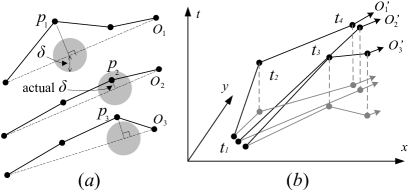
Figure 6: Trajectory Simplification

Figure 6(a) illustrates the application of DP on the trajectories in Figure 4. For $o_{1}$ trajectory, we first construct the virtual line between its end points. Since the distance between the farthest point (i.e., $p_{1}$) and the virtual line exceeds $\delta$, point $p_{1}$ will be kept in $o_{1}$’s corresponding simplified trajectory $o^{\prime}_{1}$. Regarding $o_{2}$, the distance of the furthest point (i.e., $p_{2}$) from the virtual line is below $\delta$; thus, all intermediate points are removed from $o_{2}$’s simplified trajectory. Figure 6(b) visualizes the simplified trajectories. Notice that each point in a simplified trajectory corresponds to a point in the original trajectory and is associated with a time value.

Measuring actual tolerances of simplified trajectories : We observe that an actual tolerance smaller than $\delta$ may exist so that the simplified trajectory is valid. In the example of Figure 6(a), the actual tolerance of $o^{\prime}_{2}$ is determined by the distance between $p_{2}$ and the virtual line. We formally define the actual tolerance as follows:

Definition 4

(Actual Tolerance) Let $l^{\prime}$ be a line segment in the simplified trajectory $o^{\prime}$, whose original trajectory is $o$. The actual tolerance $\delta(l^{\prime})$ of $l^{\prime}$ is defined as: $max_{t\in l^{\prime}.\tau}\;D_{PL}(o(t),l^{\prime})$. The actual tolerance $\delta(o^{\prime})$ of $o^{\prime}$ is defined as the maximum $\delta(l^{\prime})$ value over all its line segments.

The actual tolerance of each line segment $l^{\prime}$ of $o^{\prime}$ can be computed easily by examining the locations of $o$ during the corresponding time interval $l^{\prime}.\tau$. In addition, the derivation of these tolerance values can be seamlessly integrated into the DP algorithm so that the original trajectory $o$ needs not be examined again.

The actual tolerances are valuable in the sense that they can be exploited to tighten the distance computation for simplified trajectories, as we will show in the next section.

5.2 Distance Bounds for Range Search

A simplified trajectory $o^{\prime}$ may contain many omitted locations in comparison to its original trajectory $o$. Thus, it is not possible to perform (density–connected) clustering at individual time. If we generate virtual positions for the omitted points as done in CMC, there is no use for the trajectory simplification. The main challenge becomes one of performing clustering on the line segments of simplified trajectories so that each snapshot cluster (on the original trajectories) is captured by a cluster of line segments (from the simplified trajectories).

In density-based clustering techniques (e.g., DBSCAN), the core operation is $e$-neighborhood search, i.e., to find objects within distance $e$ of a given object, at a fixed time $t$. We proceed to develop the implementation of this core operation in the context of line segments. Let a line segment $l^{\prime}_{q}$ be given; our goal is then to retrieve all line segments $l^{\prime}_{i}$ whose original trajectory $o_{i}$ can possibly satisfy the condition $D(o_{q}(t),o_{i}(t))\leq e$ for some time point $t$. This way, all qualifying convoy candidates are guaranteed to be found in the filter step.

Let $o^{\prime}_{q}$ and $o^{\prime}_{i}$ be simplified trajectories of the original trajectories $o_{q}$ and $o_{i}$. At a given time $t$, the locations of $o_{q}$ and $o_{i}$ are $o_{q}(t)$ and $o_{i}(t)$. Observe that the endpoints of line segments in $o^{\prime}_{q}$ are timestamped. Let $l^{\prime}_{q}$ be a line segment in $o^{\prime}_{q}$ such that its time interval $l^{\prime}_{q}.\tau$ covers $t$. Similarly, we use $l^{\prime}_{i}$ to denote the line segment in $o^{\prime}_{i}$ satisfying $t\in l^{\prime}_{i}.\tau$. Figure 7 shows an example of two line segments $l^{\prime}_{q}$ and $l^{\prime}_{i}$.

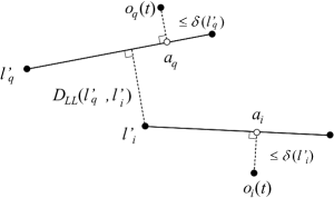
Figure 7: Trajectory Segments with Time Intervals Covering $t$

Lemma 1 establishes the relationship between distances in the original trajectories and those in the simplified trajectories.

Lemma 1

Let $o^{\prime}_{q}$ ($o^{\prime}_{i}$) be the simplified trajectory of original trajectory $o_{q}$ ($o_{i}$). Given a time $t$, let $l^{\prime}_{q}$ ($l^{\prime}_{i}$) be the line segment in $o^{\prime}_{q}$ ($o^{\prime}_{i}$) with a time interval that covers $t$.

If $D_{LL}(l^{\prime}_{q},l^{\prime}_{i})>e+\delta(l^{\prime}_{q})+\delta(l^{\prime}_{i})$ then $D(o_{q}(t),o_{i}(t))>e$.

Lemma 1 allows us to prune line segments $l^{\prime}_{i}$ during the range search of the given line segment $l^{\prime}_{q}$. Figure 8 illustrates the extended range for search over simplified line segments with error bounds. In Figure 8(a), half of the points on the original trajectory are omitted (i.e., a 50% reduction) with the given $\delta$ value. To enable correct discovery processing over the simplified trajectories (dotted lines), we enlarge the search space as shown in Figure 8(b).

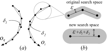
Figure 8: Range Search with Error Bounds

Notice that we still need to scan all $l^{\prime}_{i}$ whose time intervals intersect with that of $l^{\prime}_{q}$. For example, the time interval [$t_{3}$,$t_{7}$] of the second line segment of $o^{\prime}_{q}$ in Figure 9(a) intersects all of $o^{\prime}_{i}$’s line segments. To obtain better performance, we intend to prune a subset $S$ of line segments fast. During the range search of the given line segment $l^{\prime}_{q}$, Lemma 2, next, enables us to prune an non-qualifying $S$ before examining its line segments. The proofs of Lemma 1 and Lemma 2 are provided in the appendix.

Lemma 2

Let $S$ be a subset of line segments $l^{\prime}_{i}$ (from simplified trajectories). Let $\mathcal{B}(S)$ be the minimum bounding box of all segments in $S$, $S.\tau=\bigcup_{l^{\prime}_{i}\in S}l^{\prime}_{i}.\tau$, and $\delta_{max}(S)=\max_{l^{\prime}_{i}\in S}\delta(l^{\prime}_{i})$. Let line segment $l^{\prime}_{q}$ have a time interval that intersects with that of $S$, i.e., $S.\tau\cap l^{\prime}_{q}.\tau\neq\emptyset$.

If $D_{min}(\mathcal{B}(l^{\prime}_{q}),\mathcal{B}(S))>e+\delta(l^{\prime}_{q})+\delta_{max}(S)$ then
$D(o_{q}(t),o_{i}(t))>e$ holds for all $l^{\prime}_{i}\in S$.

We proceed to outline how to perform range search for $l^{\prime}_{q}$ in multiple steps by gradually tightening the condition: First, we retrieve a set of line segments $S$ whose time intervals overlap with that of $l^{\prime}_{q}$. We then apply Lemma 2 to prune non-qualifying line segments in $S$ at an early stage. Next, for each remaining line segment in $S$, we discard non-qualifying line segments by applying Lemma 1. Any surviving line segment is included in the $e$-neighborhood of the line segment $l^{\prime}_{q}$. Using this multi-step range search for line segments, we are able to perform density–connected clustering of line segments efficiently.

Figure 9: Measure of $\omega(o^{\prime}_{q},o^{\prime}_{i})$ and Time Partitioning

Extension for trajectories : So far, we have addressed range search only for line segments. In fact, it is feasible to generalize the search to apply to an entire trajectory. And by applying clustering on trajectories directly, we further reduce the cost of the filter step. As we will see in the next section, the technique below is applicable to sub-trajectories as well, enabling us to control the granularity of the filter step.

We aim to retrieve all simplified trajectories $o^{\prime}_{i}$ whose original trajectories $o_{i}$ possibly satisfy the condition $D(o_{q}(t),o_{i}(t))\leq e$ for some time $t$. In case $o^{\prime}_{q}$ and $o^{\prime}_{i}$ have disjoint time intervals (i.e., $o^{\prime}_{q}.\tau\cap o^{\prime}_{i}.\tau=\emptyset$), they cannot belong to the same convoy. Otherwise, we define their $\omega$ value as follows:

$\omega(o^{\prime}_{q},o^{\prime}_{i})=\min\{D_{LL}(l^{\prime}_{q},l^{\prime}_{i})-\delta(l^{\prime}_{q})-\delta(l^{\prime}_{i})\;|\;l^{\prime}_{i}\in o^{\prime}_{i},\;l^{\prime}_{q}\in o^{\prime}_{q},$
$l^{\prime}_{q}.\tau\cap l^{\prime}_{i}.\tau\neq\emptyset\}$.

Figure 9(a) shows an example of computing the $\omega(o^{\prime}_{q},o^{\prime}_{i})$ value between two simplified trajectories $o^{\prime}_{q}$ and $o^{\prime}_{i}$. Line segments with shared time interval are linked by dotted lines, contributing a term in the value of $\omega(o^{\prime}_{q},o^{\prime}_{i})$. If $\omega(o^{\prime}_{q},o^{\prime}_{i})>e$, no time $t$ exists such that $D(o_{q}(t),o_{i}(t))\leq e$. Otherwise, their locations in the original trajectories may be within distance $e$ for some time $t$.

5.3 The CuTS Algorithm

We first present a general overview of the CuTS (Convoy Discovery using Trajectory Simplification) algorithm, then illustrate aspects of the algorithm with examples, and finally present the details of the algorithm.

In the filter step, we first apply simplification (with tolerance $\delta$) to the original trajectories in order to obtain their simplified trajectories. We then partition the time domain (with each partition covering $\lambda$ time points) and assign the line segments of each $o^{\prime}_{i}$ to qualifying partitions. Next, we perform clustering on those line segments. Clusters across adjacent partitions with common objects are used to form convoy candidates. In the refinement step, we perform clustering of the original trajectories of the objects in each convoy candidate. The total computational cost of the CuTS algorithm is the sum of the simplification, the clustering, and the refinement costs. Our experiments in Section 7 suggest that the simplification and refinement costs are very low in practice.

To understand the filter step of CuTS better, consider Figure 9(b) where the time domain is divided into equal-length ($\lambda=4$) partitions $\mathcal{T}_{1}$ and $\mathcal{T}_{2}$ with time intervals $[t_{1},t_{4}]$ and $[t_{4},t_{7}]$, respectively. The time partition $\mathcal{T}_{1}$ contains the following line segments: $l^{1}_{1}$ and $l^{2}_{1}$ of $o^{\prime}_{1}$, $l^{1}_{2}$ of $o^{\prime}_{2}$, and $l^{1}_{3}$ and $l^{2}_{3}$ of $o^{\prime}_{3}$. Note that the line segment $l^{2}_{3}$ will be inserted into both $\mathcal{T}_{1}$ and $\mathcal{T}_{2}$ to avoid any possible false dismissal when we compute the value of $\omega(o^{\prime}_{q},o^{\prime}_{i})$ in Figure 9(a).

Algorithm description. Algorithm 2 presents the pseudocode of CuTS’s filter step. In addition to the convoy query parameters $m$, $k$, and $e$, two internal parameters $\delta$ (tolerance for trajectory simplification) and $\lambda$ (the length of each partition) also need to be specified. Those parameter values are relevant to the performance only (e.g., execution time) and do not affect the correctness. Guidelines for choosing their values will be presented in Section 7.4.

Algorithm 2 CuTS_Filter (Object set $O$, Integer $m$, Integer $k$, Distance threshold $e$)

1:  $\delta\leftarrow$ ComputeDelta($O$, $e$)

2:  for each trajectory $o_{i}\in O$ do

3:    $o^{\prime}_{i}\leftarrow$ Douglas-Peucker($o_{i},\delta$)

4:  $\lambda\leftarrow$ ComputeLambda($O$, $k$, $(\sum_{i}|o_{i}|)/(\sum_{i}|o^{\prime}_{i}|)$)

5:  $V\leftarrow\emptyset$

6:  divide the time domain into $\lambda$-length disjoint partitions

7:  for each time partition $\mathcal{T}_{z}$ (in ascending order) do

8:    $V_{next}\leftarrow\emptyset$

9:    for each $o^{\prime}_{i}$ satisfying $o^{\prime}_{i}.\tau\cap\mathcal{T}_{z}.\tau\neq\emptyset$ do

10:       insert $l^{j}_{i}\in o^{\prime}_{i}$ (intersecting time interval of $\mathcal{T}_{z}$) into $\mathcal{G}$

11:    $C\leftarrow$ TRAJ-DBSCAN($\mathcal{G},e,m$)

12:    for each convoy candidate $v\in V$ do

13:       $v.$assigned $\leftarrow$ false

14:       for each cluster $c\in C$ do

15:          if $|c\cap v|\geq m$ then

16:             $v$.assigned $\leftarrow$ true

17:             $v^{\prime}\leftarrow c\cap v$

18:             $v^{\prime}$.lifetime $\leftarrow v$.lifetime + $\lambda$

19:             $V_{next}\leftarrow V_{next}\cup v^{\prime}$

20:             $c$.assigned $\leftarrow$ true

21:       if $v$.assigned = false and $v$.lifetime$\geq k$ then

22:          $V_{cand}\leftarrow V_{cand}\cup v$

23:    for each $c\in C$ do

24:       if $c$.assigned = false then

25:          $c$.lifetime $\leftarrow\lambda$

26:          $V_{next}\leftarrow V_{next}\cup c$

27:    $V\leftarrow V_{next}$

28:  return $V_{cand}$

Lines 2–3 of the algorithm perform trajectory simplification for all objects. Next, the time domain is partitioned, each partition holding $\lambda$ consecutive time points. Time partitions are then processed iteratively in ascending order of their time. Let the current loop consider the time partition $\mathcal{T}_{z}$. The algorithm builds a polyline (i.e., a sequence of line segments) from a simplified trajectory $o^{\prime}_{i}$, which contains the line segments of $o^{\prime}_{i}$ whose time intervals intersect to $\mathcal{T}_{z}$. It then stores all the polylines from each simplified trajectory into a data structure $\mathcal{G}$. Next, density clustering is performed for the sub-trajectories in $\mathcal{G}$ (see Line 11).

The set $V$ keeps track of the convoy candidates found in previous iterations, whereas the set $V_{next}$ stores new candidates found in the current iteration. For Lines 12–20, each cluster $c\in C$ (found in the current iteration) is joined with those in $V$, as long as their intersections have at least $m$ objects. Also, candidate convoys with lifetime above $k$ are inserted into the candidate set $V_{cand}$. Clusters that cannot join with previous convoy candidates are then considered as new candidates (Lines 23–26).

Finally, Algorithm 3 contains the pseudocode of the refinement step of the CuTS algorithm. Suppose that $v$ is the convoy candidate in the candidate set $V$ that is currently being examined. We first determine the time interval $[t_{start},t_{end}]$ for $v$ and then identify the set $O^{\prime}$ of the original trajectories whose line segments appear in $v$. Finally, we apply CMC for trajectories in $O^{\prime}$, considering only time points in the interval $[t_{start},t_{end}]$.

Algorithm 3 CuTS_Refinement (Candidate set $V_{cand}$, Object set $O$, Integer $m$, Integer $k$, Distance threshold $e$)

1:  for each $v\in V_{cand}$ do

2:    $t_{start}\leftarrow$ start time of $v$

3:    $t_{end}\leftarrow$ end time of $v$

4:    $O^{\prime}\leftarrow\{o_{i}\in O\;|\;l^{j}_{i}.\tau\in v\cap l^{j}_{i}.\tau\in o_{i}\}$

5:    call CMC($O^{\prime},m,k,e$) with the time interval $[t_{start},t_{end}]$

6 Extensions of CuTS

In this section, we introduce two enhancements of CuTS. One accelerates the process of trajectory simplification and brings higher efficiency. The other shortens the search range for clustering by considering temporal information of trajectories, reducing the number of candidates after the filter step of CuTS.

6.1 Faster Trajectory Simplification - CuTS+

The Douglas-Peucker algorithm (DP) utilizes the divide-conquer technique (see Section 2.2). It is well-known that techniques built on the divide-conquer paradigm show the best performance if a given input is divided into two sub-inputs equally in each division step. Inspired by this, we modify the original DP algorithm for speeding up the simplification process, obtaining DP+.

Specifically, DP+ selects the closest point to the middle of a given trajectory among the points exceeding tolerance value $\delta$ at each approximation step. Figure 10(a) demonstrates an original trajectory having seven points, which has two intermediate points $p_{4}$ and $p_{6}$ whose distances from $\overline{p_{1}p_{7}}$ are greater than the given $\delta$ value (the gray area in the figure). The DP method selects the point having the largest distance (i.e., $\delta_{6}$); hence, the result of this division step will be as shown in Figure 10(b).

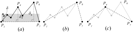
Figure 10: Comparison between DP and DP+

In contrast, our DP+ method picks the point $p_{4}$ that is the closest to the middle point of ${p_{1},p_{2},\cdots,p_{7}}$ among intermediate points exceeding $\delta$ (i.e., $p_{4}$ and $p_{6}$). This technique divides $\overline{p_{1}p_{7}}$ into two sub-trajectories $\overline{p_{1}p_{4}}$ and $\overline{p_{4}p_{7}}$, which have similar numbers of points (Figure 10(c)). Therefore, the whole process of trajectory simplification is expected to be more efficient.

Compared with DP, DP+ may have lower simplification power. In fact, each division process of DP+ does not preserve the shape of a given original trajectory well; hence, the next division process may not be as effective as that of DP. For example, in Figure 10(c), $p_{6}$ will be kept using DP+ because $D_{PL}(p_{6},\overline{p_{4}p_{7}})>\delta$, and then the simplified trajectory will be $p_{1},p_{4},p_{6},p_{7}$, whereas $p_{1},p_{6},p_{7}$ will be the result of DP in Figure 10(b).

In spite of the lower reduction, DP+ can enhance the discovery processing of CuTS in two areas. First, note that we are interested in efficient discovery of convoys in this study. As long as the search distances are bounded, faster simplification of trajectories can play a more important role in finding convoys. Second, the actual tolerances obtained by DP+ are always smaller or equal to those obtained by DP (e.g., $\delta_{4}<\delta_{6}$ in the example). This tightens the error bounds of range search for clustering, leading a more effective filter step.

We extend CuTS to CuTS+, which is built on the DP+ simplification method. All other discovery processes of CuTS+ are the same as those of CuTS.

6.2 Temporal Extension - CuTS*

Recall that CuTS applies trajectory simplification (DP) on original trajectories in the filter step. However, as we will see shortly, intermediate locations on simplified line segments cannot be associated with fixed timestamps. Consequently, the bounds on distances between line segments may not be tight, the result being that overly many convoy candidates can be produced in the filter step. This may yield a more expensive refinement step.

In this section, we extend CuTS to CuTS* by considering temporal aspects for both the trajectory simplification and the distance measure on simplified trajectories. This enables us to tighten distance bounds between simplified trajectories, improves the effectiveness of the filter step.

Comparison between DP and DP*: We discussed the differences between the two trajectory simplification techniques DP [11] and DP* [23] in Section 2.2. In Figure 3(b), DP* translates the time ratio of $p_{2}$ between $p_{1}$ and $p_{3}$ into a location $p^{\prime}_{2}$ on the line segment $\overline{p_{1}p_{3}}$. Since $p_{2}$ exceeds the $\delta$ range of $p^{\prime}_{2}$, the point $p_{2}$ is kept in the simplified trajectory $o^{\prime}_{1}$, which is different from DP.

From the example, we can see that DP* has a lower vertex reduction ratio for trajectories. Nevertheless, DP* permits us to derive tighter distance measures between trajectory segments, improving the overall effectiveness of the filter step.

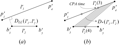
Figure 11: Different Distance Measures of Trajectory Segments

Figure 11(a) shows two simplified line segments $l^{\prime}_{1}$ and $l^{\prime}_{2}$, obtained from DP. Here, $l^{\prime}_{1}$ has the endpoints $p^{\prime}_{1}$ and $p^{\prime}_{4}$, corresponding to its locations at times $t_{1}$ and $t_{4}$. Similarly, $l^{\prime}_{2}$ has endpoints $b^{\prime}_{3}$ and $b^{\prime}_{5}$, corresponding to its locations at times $t_{3}$ and $t_{5}$. The shortest distance between $l^{\prime}_{1}$ and $l^{\prime}_{2}$ is given by $D_{LL}(l^{\prime}_{1},l^{\prime}_{2})$.

Figure 11(b) contains simplified line segments from DP*. Since DP* captures the time ratio in the simplified line segment, we are able to derive the locations $l^{\prime}_{1}(3)$ on $l^{\prime}_{1}$ and $l^{\prime}_{2}(4)$ on $l^{\prime}_{2}$. Let $l^{\prime}_{p}=\{p_{u},p_{v}\}$ be a simplified line segment having a time interval $l^{\prime}_{p}.\tau=[u,v]$. The location of $l^{\prime}_{p}$ at a time $t\in[u,v]$ is defined as:

$$l^{\prime}_{p}(t)=p_{u}+\frac{t-u}{v-u}(p_{v}-p_{u})$$

Note that the terms $l^{\prime}_{p}(t)$, $p_{u}$, and $(p_{v}-p_{u})$ are 2D vectors representing locations.

Before defining $D_{*}(l^{\prime}_{1},l^{\prime}_{2})$ formally, we need to introduce the time of the Closest Point of Approach, called the CPA time ($t_{CPA}$) [6]. This is the time when the distance between two dynamic objects is the shortest, considering their velocities. Let $l^{\prime}_{q}=\{q_{w},q_{x}\}$ be another simplified line segment during $l^{\prime}_{q}.\tau=[w,x]$. The CPA time of $l^{\prime}_{p}$ and $l^{\prime}_{q}$ is computed by :

$$t_{CPA}=\frac{-(p_{u}-q_{w})\cdot(l^{\prime}_{p}(t)-l^{\prime}_{q}(t))}{|l^{\prime}_{p}(t)-l^{\prime}_{q}(t)|^{2}}$$

where, $l^{\prime}_{q}(t)$, $q_{w}$, and $(q_{w}-q_{x})$ are also location vectors.

Observe that the common interval of $l^{\prime}_{1}$ and $l^{\prime}_{2}$ is $[t_{3},t_{4}]$ (gray area in Figure 11(b)). The tightened shortest distance $D_{*}(l^{\prime}_{1},l^{\prime}_{2})$ between them is computed as :

$$D_{*}(l^{\prime}_{1},l^{\prime}_{2})=D(l^{\prime}_{1}(t_{CPA}),l^{\prime}_{2}(t_{CPA}))\hskip 14.22636ptt_{CPA}\in(l^{\prime}_{1}.\tau\cap l^{\prime}_{2}.\tau)$$

When their time intervals do not intersect, i.e., $l^{\prime}_{1}.\tau\cap l^{\prime}_{2}.\tau=\emptyset$, their distance is set to $\infty$ .

Clearly, $D_{*}(l^{\prime}_{1},l^{\prime}_{2})$ is longer than $D_{LL}(l^{\prime}_{1},l^{\prime}_{2})$; hence, the line segments in Figure 11(b) have a lower probability of forming a cluster together than do those in Figure 11(a). These tightened distance bounds improve the effectiveness of the filter step.

Distance bounds for DP* simplified line segments: Using the notations from Lemma 1, we derive the counterpart that uses the tightened distance $D_{*}$ between line segments (as opposed to the distance $D_{LL}$). Lemma 3 establishes the relationship between distances in original trajectories and those in simplified trajectories (obtained by DP*). The proof is provided in the appendix.

Lemma 3

Suppose that $o^{\prime}_{q}$ ($o^{\prime}_{i}$) is the simplified trajectory (from DP*) of the original trajectory $o_{q}$ ($o_{i}$). Given a time $t$, let $l^{\prime}_{q}$ ($l^{\prime}_{i}$) be the line segment in $o^{\prime}_{q}$ ($o^{\prime}_{i}$) with time interval covering $t$.

If $D_{*}(l^{\prime}_{q},l^{\prime}_{i})>e+\delta(l^{\prime}_{q})+\delta(l^{\prime}_{i})$ then $D(o_{q}(t),o_{i}(t))>e$.

CuTS* algorithm for convoy discovery: We develop an enhanced algorithm, called CuTS*, to exploit the above tightened distance bounds for query processing. Two components of CuTS need to be replaced. First, CuTS* applies DP* for the trajectory simplification. Second, during density clustering in the filter step, Lemma 3 is utilized in the range search operations (as opposed to Lemma 1). The above modifications improve the effectiveness of the filter step in CuTS*. The following table summarizes the key components of CuTS and its extensions.

Method	CuTS	CuTS+	CuTS*
simplification	DP [11]	DP+ [Section 6.1]	DP* [23]
distance function	$D_{LL}$	$D_{LL}$	$D_{*}$

7 Experiments

In this experimental study, we first compare the discovery efficiency between CMC, which is an adaption of a moving-clustering algorithm (MC2) [19] for our convoy discovery problem, and the CuTS family (CuTS, CuTS+, and CuTS*). We then analyze the performance of each method of the CuTS family while varying the settings of their key parameters.

We implemented the above algorithms in the C++ language on a Windows Server 2003 operating system. The experiments were performed using an Intel Xeon CPU 2.50 GHz system with 16GB of main memory.

7.1 Dataset and Parameter Setting

For studying the performance of our methods in a real-world setting, we used several real datasets that were obtained from vehicles and animals. Due to the different object types, their trajectories have distinct characteristics, such as the frequency of location sampling and data distributions. The details of each dataset are described as follows:

Truck: We obtained 276 trajectories of 50 trucks moving in the Athens metropolitan area in Greece [2]. The trucks were carrying concrete to several construction sites for 33 days while their locations were measured. To be able to find more convoys, we regarded each trajectory as a distinct truck’s trajectory and removed the day information from the data. Thus, the dataset became 276 trucks’ movements on the same day.

Cattle: To reduce a major cost for cattle producers, a virtual fencing project in CSIRO, Australia studied managing herds of cattle with virtual boundaries. We obtained 13 cattle’s movements for several hours from the project. Their locations were provided by GPS-enabled ear–tags every second. A distinguishable aspect of this dataset is its very large number of timestamps.

Car: Normal travel patterns of over 500 private cars were analyzed for building reasonable road pricing schemes in Copenhagen, Denmark. We obtained 183 cars’ trajectories during one week [3]. Trajectories in this dataset had very different lengths.

Taxi: The GPS logs of 500 taxis in Beijing, China were recorded during a day and studied in Institute of Software, Chinese Academy of Sciences. The locations of the trajectories were sampled irregularly. For example, some taxis reported their locations every three minutes, while some did it once in several minutes.

In our experiments, we defined a convoy as containing at least 3 objects (except Cattle due to the small number of objects) that travel closely for 3 minutes (i.e., $m=3$ and $k=180$). We also adjusted the values of neighborhood range $e$ to be able to find 1 to 100 convoys for each dataset. To perform convoy discovery using our main methods (CuTS, CuTS+, and CuTS*), we still need to determine two key parameters, namely the tolerance value ($\delta$) for trajectory simplification and the length of time partition ($\lambda$). These parameter values were computed by our guidelines that will be discussed in Section 7.4.

Table 3 provides (i) detailed information of each dataset, (ii) the settings of the parameters to be used throughout our experiments, and (iii) the number of convoys discovered by our proposed methods with the parameters.

	Truck	Cattle	Car	Taxi
number of objects ($N$)	267	13	183	500
time domain length ($T$)	10586	175636	8757	965
average trajectory length	224	175636	451	82
data size (points)	59894	2283268	82590	41144
number of convoy objects ($m$)	3	2	3	3
convoy lifetime ($k$)	180	180	180	180
neighborhood range ($e$)	8	300	80	40
simplification tolerance ($\delta$)	5.9	274.2	63.4	31.5
time partition length ($\lambda$)	4	36	24	4
number of convoys discovered	91	47	15	4

Table 3: Settings for Experiments

7.2 CMC vs. The CuTS Family

First, we compared the efficiency of CMC versus the CuTS family. Over all the datasets, the CuTS family was 3.9 times (at least) to 33.1 times (at most) faster than CMC, as seen in Figure 12, and especially CuTS* had the highest efficiency. The performance differences were more obvious in the Car and the Taxi datasets though their data sizes (total number of points) were less than 10% of Cattle’s data size. Since those two datasets had many numbers of missing points and different lifetimes of each trajectory, CMC incurred extra computational cost to make virtual points for those missing times to measure density-connection correctly (see Section 4). It also caused a considerable growth of the actual data size for the discovery processing. Notice that our main methods, the CuTS family, can perform the discovery without any extra processing regardless of the number of missing points.

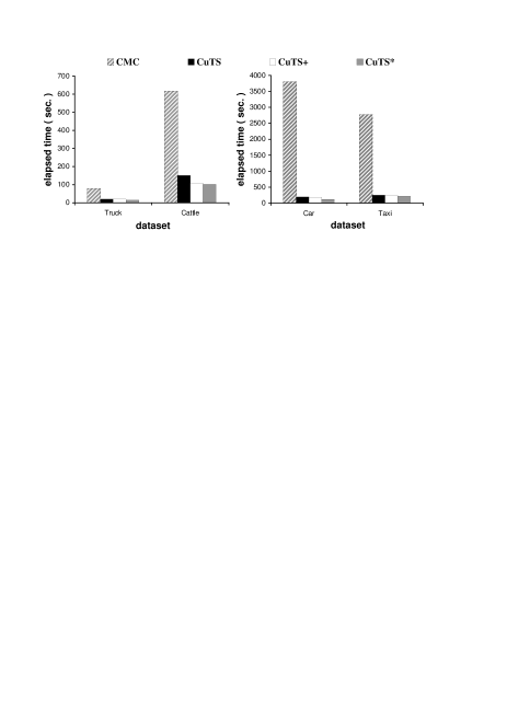
Figure 12: Comparisons of Query Processing Time

In Figure 13, we report on the elapsed times of each method of the CuTS family for the Cattle and Taxi datasets (magnified views of the results in Figure 12). For brevity, we show the two most distinctive results only. In the results for the Cattle dataset, the simplification cost dominates for all the methods. In general, convoy processing is more sensitive to the number of objects $N$ than to the number of timestamps $T$ since the clustering method (DBSCAN) has $O(N^{2})$ computational cost ($O(N\cdot\log N)$ with a spatial index). The Cattle dataset has only 13 objects, and the cost of each clustering is very low though it is performed $T$ times. As a result, the total discovery times are more influenced by the simplification process than the filtering and refinement steps.

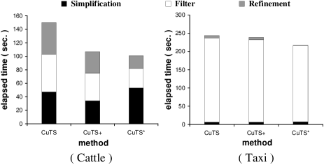
Figure 13: Analysis of Query Processing Cost

The reason why each simplification method has different efficiency will be studied in Section 7.3. Recall that, although the CuTS family needs much time for trajectory simplification on the Cattle dataset, their total discovery times are still much lower than those of CMC in the previous experiments.

Another interesting observation found with the Cattle data is that CuTS+ has not only faster trajectory simplification, but also lower refinement cost. This is because DP+ as used in CuTS+ has not only higher efficiency of simplification, but also tighter error bounds than DP as used by CuTS, as described in Section 6.1.

Compared to the Cattle data, trajectory simplification had very low computational cost on the Taxi dataset. As the Taxi dataset has a short $T$ but a larger $N$, the clustering cost dominates the discovery time. In addition, since the number of convoy candidates was small for this data (will be shown in the next experiments), only little refinement was necessary.

For the other two datasets, the composition of computational time was about 70%-80% for filtering (around 5%-15% for trajectory simplification) and 20%-30% for refinement. Therefore, it is very reasonable to ‘invest’ some time in trajectory simplification.

We also studied the effect of using the actual tolerance for the range search of clustering. When we perform the trajectory simplification, we use the tolerance value $\delta$, named the global tolerance here. The key process of the simplification is to remove intermediate points whose distances from the virtual line linking two end points of the original trajectory do not exceed $\delta$. Any distance of those removed points (i.e., actual tolerance) is always smaller than or equal to the global tolerance (see Section 5.1). The actual tolerance is useful for range search since the search area should be reduced.

Figure 14: Effect of Actual Tolerance

Figure 14(a) demonstrates the filtering power of the global and actual tolerances for CuTS*. We omit the results for CuTS and CuTS+ because they are similar. As shown, the number of candidates after the filtering step decreases considerably when we use the actual tolerance. The advantage of the improved filtering by the actual tolerance is reflected in the efficiency of convoy discovery as shown in Figure 14(b). Yet, the effect is relatively small on the Truck and the Taxi datasets. This is because some candidates that do not need much computation for the refinement step are pruned when using the actual tolerance. We present a more precise way of measuring the filter’s effectiveness in the following section.

7.3 CuTS vs. CuTS+ vs. CuTS*

We have already discussed different techniques for trajectory simplification. The difference between the original Douglas-Peucker algorithm (DP) and its temporal extension DP* was covered in Section 2.2. We also developed a DP variant, named DP+, in Section 6.1. It is of interest to compare the performance of those methods.

Figure 15(a) illustrates the differences of their reduction power for the Cattle dataset. We skip the results for the other datasets because they show similar trends. With the same values of tolerance, DP shows higher reduction rates than does DP*. This is natural since DP* uses the time-ratio distance to approximate points, which is always equal to or greater than the perpendicular distance of DP (see Section 6.2). Furthermore, the vertex reduction of DP+ is lower than that of DP. This is because DP+ does not preserve the shapes of the original trajectories well when compared to DP. This aspect was explained in Section 6.1.

Figure 15: Comparison of Trajectory Simplification Methods

In Figure 15(b), DP+ exhibits the fastest elapsed time among the methods because of its more effective division process. An interesting observation of the figure is that the efficiency of all the methods grows as reduction ratios increase. Recall that all the methods utilize the divide-and-conquer paradigm, which divides an input trajectory until no point exceeds a given $\delta$. With a larger value of $\delta$, their division processes are likely to meet the ‘end’ quicker. For this reason, DP* also performs slower than the other methods (lower reduction power than the others).

Next, we compare the discovery effectiveness and efficiency for the CuTS family. Given very large values of $e$ and $\delta$, the CuTS family may produce one candidate containing all actual results after the filter step and then the candidate may be divided into a large number of real convoys through the refinement step. Thus, we cannot use the count of false positives as a measure of the filters’ effectiveness for our study.

Instead, we calculate refinement unit that represents the computational cost of candidates for the refinement step, which reflects the filtering power of each method effectively. Specifically, the clustering cost of the convoy objects in each candidate is computed and then multiplied by the candidate’s lifetime. As mentioned earlier, the computational cost of clustering is either $O(N^{2})$ without index or $O(N\cdot\log N)$ with a spatial index. To clarify the differences of each filter method, we considered the clustering without index support in our experiments. For example, if a convoy candidate has 3 objects and its lifetime is 2, the refinement unit is $3^{2}\times 2=18$. Next, we aggregate each candidate’s unit to obtain the total refinement unit.

Figure 16: Effect of Simplification Tolerance ($\delta$)

Figure 16 demonstrates the filtering power and the total discovery times for the CuTS family when varying $\delta$. We omit the results for the Truck and Cattle datasets, but those two datasets will be used in the next experiments. As expected, CuTS* has the lowest refinement unit for both datasets, which yields the highest efficiency as well. In addition, CuTS+ has a better filtering effectiveness than does CuTS. As discussed in Section 6.1, the actual tolerances obtained by DP+ of CuTS+ are always smaller or equal to those obtained by DP of CuTS. As a result, the search range for clustering is reduced, and the filtering power grows in the figure.

Another observation found in Figure 16, for all members of the CuTS family is that both the filters’ effectiveness and the discovery efficiency decrease as the tolerance value increases as the $\delta$ values affect not only the result of trajectory simplification, but also that of range search for clustering.

Although the total elapsed times of the Car data grow steadily with increasing $\delta$, those of the Taxi data stay almost constant or increase only very slightly. This is because the enlargement of the search range is not sufficient to find more actual convoys with respect to the given parameters. From this point, we can infer that the trajectories of the Taxi dataset are distributed relatively uniformly, and thus the number of taxis traveling together within a given (reasonable) distance is low.

Figure 17: Effect of Time Partitioning ($\lambda$)

Lastly, we study how the size of the time partition $\lambda$ affects the results of the convoy discovery. In fact, a large value of $\lambda$ yields an ineffective filtering step, whereas more times of clustering are performed with a small value of $\lambda$ (see Section 5.3). In the Truck dataset of Figure 17, CuTS* shows better performance than the other methods regardless of the $\lambda$ value. Also, both the effectiveness of the filters and the efficiency of the discovery process decrease when $\lambda>10$ for this dataset, for all methods of the CuTS family.

On the other hand, the discovery efficiency of the CuTS family declines over the Cattle dataset when $\lambda<30$, although their refinement unit increases steadily in the same range of $\lambda$. This implies that an appropriate $\lambda$ value is influenced by not only the filter’s effectiveness, but also another fact, possibly the length of trajectories since the average size of Cattle’s trajectories is very large.

Another interesting observation found in the Cattle dataset is that CuTS+ has similar efficiency to CuTS*, and it is even faster for $\lambda\geq 50$. As seen in Figure 13, trajectory simplification is the key part of the total discovery time on this dataset. Therefore, faster trajectory simplification (i.e., DP+) plays a more important role in the discovery efficiency in this case.

7.4 Parameter Determination of CuTS

Proper values of $\delta$ and $\lambda$ may be difficult to find in some applications since they are dependent on the data characteristics. In this section, we provide guidelines for determining settings for these parameters. Note that the parameters do not affect the correctness of discovery results, but only affect execution times.

Tolerance for trajectory simplification ($\delta$) : It is obvious that a larger value of $\delta$ for DP of CuTS achieves a higher reduction result of trajectory simplification. On the other hand, a large $\delta$ value is also used for the range search of clustering in the CuTS algorithm; hence, the filter step of CuTS may not be tight enough to prune many unnecessary candidate objects. In this tradeoff, our goal is to find a value satisfying the following conditions : (i) the original trajectories become well simplified, and (ii) the distance bounds are sufficiently tight, implying an effective filter process.

As the first step, we perform the original DP algorithm over a trajectory with $\delta=0$. In each step of the division process (see details in Sections 2.2 and 5.1), we store the actual tolerance values in ascending order. Since $\delta=0$, the process continues until all intermediate points of the original trajectory are tested.

In the next step, we find the largest variance between two adjacent tolerances stored, and then select the smaller one of those two tolerances. For example, assume that the DP method with $\delta=0$ results in the 10 actual tolerance values $\delta_{1},\delta_{2},\cdots,\delta_{10}$ in Figure 18(a) through the first step. The difference in the tolerance values is the largest between $\delta_{5}$ and $\delta_{6}$. We then select $\delta_{5}$ as a tolerance value $\delta_{s}$. This selection is performed as long as $\delta_{i}<e$ (the dark gray bars in Figure 18(a)). From our experimental studies, we found out that the filtering power of the CuTS family decreases considerably on some datasets when we pick $\delta_{i}>e$.

Lastly, we perform the above steps for a sufficient time (e.g., 10% of $N$) and average the $\delta_{s}$ values selected to obtain a final $\delta$ for the processing of trajectory simplification.

The idea behind this method is to find a relatively small $\delta$ value that achieves a reasonable reduction through simplification. In the figure, if we pick $\delta_{10}$ and apply it to the trajectory simplification, the reduction ratio will be nearly 100%. Likewise, the use of $\delta_{5}$ for the simplification is able to yield around a 50% reduction although it does not necessarily follow the same division processes with $\delta=0$ as the first step. If we pick $\delta_{6}$ instead, it may bring (approximately) 60% of trajectory reduction, which is slightly higher than 50%. However, the value of $\delta_{6}$ is much bigger than $\delta_{5}$, and the effectiveness of range search can decrease dramatically.

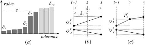
Figure 18: Value Selection of $\delta$ and $\lambda$

Length of time partition ($\lambda$) : In Section 5.3, we discussed about dividing the time domain $T$ into time partitions for discovery processing, each of which has length $\lambda$. If a time partition $\mathcal{T}_{i}$ has a large value for $\lambda$, many line segments of a simplified trajectory within $\mathcal{T}_{i}$ form a long polyline. Thus, the distances among those polylines become small, and many objects are likely to form a cluster together, leading to ineffective filtering results. In contrast, a small value of $\lambda$ involves many computationally expensive clustering processes ($T/\lambda$ times).

Suppose that $o^{\prime}_{1}$ and $o^{\prime}_{2}$ in Figure 18(b) are simplified trajectories. In the figure, one clustering with $\lambda_{1}$ is obviously more efficient than two processes with $\lambda_{0}$ because both cases have the same minimum distance between $o^{\prime}_{1}$ and $o^{\prime}_{2}$. From this example, we can infer the value of $\lambda_{1}$ by computing $\frac{|o^{\prime}|}{|o|}\times o.\tau$, where $|o|$ ($|o^{\prime}|$) is the number of points in the trajectory $o$ ($o^{\prime}$) and $o.\tau$ is the time interval of $o$.

In practice, however, there may be some time points that one (simplified) trajectory has, but others do not have, such as $p^{\prime}_{2}$ on $o^{\prime}_{3}$ in Figure 18(c). Using the $\lambda_{1}$ for this case should not keep the filter’s ‘good’ effectiveness, and we need to lower the $\lambda_{1}$ value. We can roughly estimate the probability that such case occurs by looking at how densely a trajectory exits in the time space $T$. Notice that each trajectory may have a different length ($o.\tau$) and may appear and disappear at any arbitrary time points in $T$. Thus, the density of the trajectory is obtained by $o.\tau/T$. Finally, the probability that an object has an intermediate time point within $\lambda_{1}$ is $(\lambda_{1}-2)\times o.\tau/T$. Together, we obtain $\lambda=\lambda_{1}-(\lambda_{1}-2)\times o.\tau/T$, rewriting $\lambda=o.\tau\times(\frac{|o^{\prime}|}{|o|}\times(1-\frac{o.\tau}{T})+\frac{2}{T})$.

So far, we have considered the computation of $\lambda$ for a single object. To obtain an overall value of $\lambda$, we perform the above computation for all objects and average the values. Note that all the statistics for this $\lambda$ computation can be easily gathered when a dataset is loaded into the system (or one scan for disk-based implementations).

Although this method does not capture the distribution of a dataset precisely, the value of $\lambda$ is quickly obtained and brings reasonable efficiency of the CuTS family.

8 Conclusion

Discovering convoys in trajectory data is a challenging problem, and existing solutions to related problems are ineffective at finding convoys. This study formally defines a convoy query using density-based notions, and it proposes four algorithms for computing the convoy query. Our main algorithms (CuTS, CuTS+, and CuTS*) use line simplification methods as the foundation for a filtering step that effectively reduces the amounts of data that need further processing. In order to ensure that the filters do not eliminate convoys, we bound the errors of the discovery processing over the simplified trajectories. Through our experimental results with real datasets, we found that CuTS* showes the best performance. CuTS+ also performes well when the given trajectories have a small number of objects and long histories.

Appendix A Proofs of Lemmas

A.1 Proof of Lemma 1

Consider the example of Figure 7. To prove the lemma by contradiction, assume the following equation holds:

$$D(o_{q}(t),o_{i}(t))\leq e$$

Since $l^{\prime}_{q}$ is a line segment (with actual tolerance $\delta(l^{\prime}_{q})$) in the simplified trajectory $o^{\prime}_{q}$, there exists a location $a_{q}$ on $l^{\prime}_{q}$ such that $D(a_{q},o_{q}(t))\leq\delta(l^{\prime}_{q})$. Similarly, there exists a location $a_{i}$ on $l^{\prime}_{i}$ such that $D(a_{i},o_{i}(t))\leq\delta(l^{\prime}_{i})$. Due to the triangular inequality,

$$D(a_{q},a_{i})\leq D(a_{q},o_{q}(t))+D(o_{q}(t),o_{i}(t))+D(o_{i}(t),a_{i})$$

Combining the inequalities, we obtain:

$$D(a_{q},a_{i})\leq\delta(l^{\prime}_{q})+e+\delta(l^{\prime}_{i})$$ (1)

On the other hand, $a_{q}$ ($a_{i}$) is a location on line segment $l^{\prime}_{q}$ ($l^{\prime}_{i}$). Hence, equation (2) holds

$$D_{LL}(l^{\prime}_{q},l^{\prime}_{i})\leq D(a_{q},a_{i})$$ (2)

From the last two inequalities (1) and (2), we get:

$$D_{LL}(l^{\prime}_{q},l^{\prime}_{i})\leq e+\delta(l^{\prime}_{q})+\delta(l^{\prime}_{i})$$ (3)

Therefore, the resulting contradiction of (3) proves Lemma 1.

A.2 Proof of Lemma 2

Note that for all $l^{\prime}_{i}\in S$, we have $\delta_{max}(S)\geq\delta(l^{\prime}_{i})$ and
$D_{min}(\mathcal{B}(l^{\prime}_{q}),\mathcal{B}(S))\leq D_{LL}(l^{\prime}_{q},l^{\prime}_{i})$. If the following equation satisfies:

$$D_{min}(\mathcal{B}(l^{\prime}_{q}),\mathcal{B}(S))>e+\delta(l^{\prime}_{q})+\delta_{max}(S)$$

then, the next equation must also hold:

$$D_{LL}(l^{\prime}_{q},l^{\prime}_{i})>e+\delta(l^{\prime}_{q})+\delta(l^{\prime}_{i})$$

The rest of this proof follows directly from Lemma 1.

A.3 Proof of Lemma 3

Since $l^{\prime}_{q}$ is a line segment (with actual tolerance $\delta(l^{\prime}_{q})$) in the simplified trajectory $o^{\prime}_{q}$ , the location $l^{\prime}_{q}(t)$ meets:

$$D(l^{\prime}_{q}(t),o_{q}(t))\leq\delta(l^{\prime}_{q})$$

Similarly, the location $l^{\prime}_{i}(t)$ satisfies:

$$D(l^{\prime}_{i}(t),o_{i}(t))\leq\delta(l^{\prime}_{i})$$

In addition, we have:

$$D_{*}(l^{\prime}_{q},l^{\prime}_{i})\leq D(l^{\prime}_{q}(t),l^{\prime}_{i}(t))$$

The logic of the remainder of the proof is the same as in the proof of Lemma 1.

Appendix B Additional Experiments

B.1 MC vs. CMC

In this experiment, we intend to demonstrate empirically that methods for the discovery of moving clusters cannot be used to compute convoys directly (see Section 2.1). Specifically, we study the discovery accuracies of convoys by a solution for moving cluster (MC2). MC2 reports results of the convoy query if the portion of common objects in any two consecutive clusters $c_{1}$ and $c_{2}$ is not below a given threshold parameter $\theta$, i.e., $\frac{|c_{1}\cap c_{2}|}{|c_{1}\cup c_{2}|}\geq\theta$.

Let $R_{m}$ be a result set of convoys discovered by MC2 and $R_{c}$ be another set obtained by CMC (or CuTS). We measure the proportions of false positives in Figure 19(a) by verifying whether each convoy $v\in R_{m}$ satisfies the query condition with respect to $m$, $k$, and $e$ using the results of CMC (i.e., $(\frac{|R_{m}-R_{c}|}{|R_{m}|})\times 100$). Likewise, false negatives in Figure 19(b) are computed by $(\frac{|R_{c}-R_{m}|}{|R_{c}|})\times 100$).

Figure 19: Discovery Quality of the MC method for Convoys

In fact, MC2 reported bigger numbers of convoys than what CMC does because MC2 does not have the lifetime constraint $k$. This feature was especially obvious for the Cattle dataset that is larger than the others. As a result, the proportions of actual convoys in the result set were very low, and the numbers of false positives were very high in Figure 19(a). For the other datasets, false positives went up as the $\theta$ value grew since the number of convoys reported by MC2 also increased. Let $\theta_{c_{1}c_{2}}$ be a ratio of common objects between two snapshot clusters $c_{1}$ and $c_{2}$. Assume that there are four consecutive snapshot clusters $c_{1},c_{2},c_{3},$ and $c_{4}$, and $\theta_{c_{1}c_{2}}=1.0,\theta_{c_{2}c_{3}}=0.8,\theta_{c_{3}c_{4}}=1.0$. If we set the value of $\theta$ to be equal to or smaller than 0.8, one moving cluster having all the snapshot clusters will be reported (say $MC_{c_{1}c_{2}c_{3}c_{4}}$). In contrast, when $\theta>0.8$, MC2 will discover two moving clusters $MC_{c_{1}c_{2}}$ and $MC_{c_{3}c_{4}}$. Therefore, a higher $\theta$ value may produce a larger number of moving clusters as convoy results.

Even though MC2 returns many convoys, the result set did not necessarily contain all actual convoys. We investigate this aspect by computing false negatives in Figure 19(b). In general, the number of false negatives increases as the $\theta$ value increases because the number of convoys discovered by MC2 also increases. Note that if many actual convoys exist for different parameter settings, the proportions of both false positives and false negatives may increase considerably. Therefore, the use of moving cluster methods for convoy discovery is ineffective and unreliable.

References

- [1] Inrix, Inc. Smart Dust Network. http://www.inrix.com/techdustnetwork.asp.
- [2] http://www.rtreeportal.org/
- [3] http://daisy.aau.dk/
- [4] H. Jeung, H. T. Shen, and X. Zhou. Convoy Queries in Spatio-Temporal Databases. In ICDE, pp. 1457–1459, 2008.
- [5] G. Al-Naymat, S. Chawla, and J. Gudmundsson. Dimensionality reduction of long duration and complex spatio-temporal queries. In ACM SAC, pp. 393–397, 2007.
- [6] S. Arumugam and C. Jermaine. Closest-point-of-approach join for moving object histories. In ICDE, p. 86, 2006.
- [7] P. Bakalov, M. Hadjieleftheriou, and V. J. Tsotras. Time relaxed spatiotemporal trajectory joins. In ACM GIS, pp. 182–191, 2005.
- [8] H. Cao, O. Wolfson, and G. Trajcevski. Spatio-temporal data reduction with deterministic error bounds. VLDBJ, 15(3): 211–228, 2006.
- [9] L. Chen and R. T. Ng. On the marriage of lp-norms and edit distance. In VLDB, pp. 792–803, 2004.
- [10] L. Chen, M. T. Özsu, and V. Oria. Robust and fast similarity search for moving object trajectories. In SIGMOD, pp. 491–502, 2005.
- [11] D. Douglas and T. Peucker. Algorithms for the reduction of the number of points required to represent a line or its character. The American Cartographer, 10(42):112–123, 1973.
- [12] M. Ester, H.-P. Kriegel, J. Sander, and X. Xu. A density-based algorithm for discovering clusters in large spatial databases with noise. In SIGKDD, pp. 226–231, 1996.
- [13] J. Gudmundsson and M. van Kreveld. Computing longest duration flocks in trajectory data. In ACM GIS, pp. 35–42, 2006.
- [14] J. Gudmundsson, M. van Kreveld, and B. Speckmann. Efficient detection of motion patterns in spatio-temporal data sets. In ACM GIS, pp. 250–257, 2004.
- [15] D. Gunopoulos. Discovering similar multidimensional trajectories. In ICDE, pp. 673–684, 2002.
- [16] J. Hershberger and J. Snoeyink. Speeding up the douglas-peucker line-simplification algorithm. In International Symposium on Spatial Data Handling, pp. 134–143, 1992.
- [17] C. S. Jensen, D. Lin, and B. C. Ooi. Continuous clustering of moving objects. IEEE TKDE, 19(9): 1161–1174, 2007.
- [18] S. Jeong, N. Paton, A. Fernandes, and T. Griffiths. An experimental performance evaluation of spatiotemporal join strategies. Transactions in GIS, 9(2):129–156, 2005.
- [19] P. Kalnis, N. Mamoulis, and S. Bakiras. On discovering moving clusters in spatio-temporal data. In SSTD, pp. 364–381, 2005.
- [20] J. Lee, J. Han, and K.-Y. Whang. Trajectory clustering: A partition-and-group framework. In SIGMOD, pp. 593–604, 2007.
- [21] Y. Li, J. Han, and J. Yang. Clustering moving objects. In SIGKDD, pp. 617–622, 2004.
- [22] Z. Li. An algorithm for compressing digital contour data. The Cartographic Journal, 25(2): 143–146, 1988.
- [23] N. Meratnia and R. A. de By. Spatiotemporal compression techniques for moving point objects. In EDBT, pp. 765–782, 2004.
- [24] M. Spiliopoulou, I. Ntoutsi, Y. Theodoridis, and R. Schult. Monic: modeling and monitoring cluster transitions. In SIGKDD, pp. 706–711, 2006.
- [25] B. Yi, H. V. Jagadish, and C. Faloutsos. Efficient retrieval of similar time sequences under time warping. In ICDE, pp. 201–208, 1998.
- [26] P. Zhou, D. Zhang, B. Salzberg, G. Cooperman, and G. Kollios. Close pair queries in moving object databases. In ACM GIS, pp. 2–11, 2005.