We do parametric calculations to elucidate multi-terminal electron transport properties through a molecular system where a single phenalenyl molecule is attached to semi-infinite one-dimensional metallic leads. A formalism based on the Green’s function technique is used for the calculations while the model is described by tight-binding Hamiltonian. We explore the transport properties in terms of conductance, reflection probability as well as current-voltage characteristic. The most significant feature we articulate is that all these characteristics are very sensitive to the locations where the leads are connected and also the molecule-to-lead coupling strengths. The presence of other leads also has a remarkable effect on these transport properties. We study these phenomena for two-, three- and four-terminal molecular systems. Our numerical study may be utilized in designing tailor-made molecular electronic devices.

PACS No.: 73.23.-b; 73.63.-b; 81.07.Nb; 85.65.+h

Keywords: Phenalenyl molecule; Multi-terminal conductance; Reflection probability; $I$-$V$ characteristic.

1 Introduction

Speed of growth of molecular electronics is being accelerated more and more as it has brought together scientists and engineers from various disciplines. The reason behind this attraction is inscribed into its smallness of size with wonderful electronic properties. In addition, several other properties such as magnetic, optical, etc., have been recognized in different molecules, which may be utilized in artificially tailored devices that are not possible with conventional materials [1]. The concept of electron transport which emerged first in the theoretical work of Aviram and Ratner in $1974$ [2] has opened a new era in the field of nanoscience. But at that time any type of measurement in such a small scale was a long-sought goal. Study at molecular scale level is not a simple one as we cannot avoid the effect of interface to the external electrodes. However, the progress in the theoretical works [3] was continuing, which bestowed inspirations to the experimentalists to take such task as a challenge. Now with the advancement in nanotechnology, it is possible to investigate several transport properties not only through a group of molecules [4] but also through a single molecule [5]. This single molecular electronics may play a key role in designing nanoelectronic circuits. For this we have to have a thorough understanding of the electronic transport processes at this molecular scale level [6, 7, 8, 9, 10, 11]. Many problems are yet to be solved to make this field much more reliable. Therefore, the electron transport in molecular systems is an open area and detailed investigations of molecular transport are still needed.

All these works we have referred above are related to two-terminal electron transports. We can also analyze various transport phenomena of a multi-terminal system, which was first addressed by Büttiker [12]. The Büttiker formalism, which is an extension of the Landauer two-terminal conductance formula, is a very simple and elegant way to divulge the transport mechanism in terms of various transmission probabilities. There are several pioneering works [13, 14, 15, 16, 17] based on this formalism, which are very interesting from the theoretical as well as experimental point of view.

Several ab initio methods [18, 19, 20, 21] are there which may be utilized to study electron transport properties through molecular junctions. At the same time, tight-binding model has been extended to density functional theory (DFT) for transport calculations [22]. But in case of molecular systems, the investigations based on this theory (DFT) have some quantitative discrepancies compared to the experimental predictions. More over, these ab initio theories are computationally very expensive. To avoid this we do model calculations by using a simple tight-binding framework.

In the present article we do a theoretical study of multi-terminal electron transport through a single phenalenyl molecule [23, 24] attached to semi-infinite one-dimensional ($1$D) metallic leads. We do exact numerical calculations based on single particle Green’s function formalism [25, 26] to evaluate conductance, reflection probability and current-voltage characteristics. Quite interestingly, we show that the positions where the leads are connected to the molecule as well as the presence of other leads have eloquent effects on these transport properties. More over, these characteristics are also influenced significantly by the molecule-to-lead coupling strengths. These aspects can be utilized in designing nano-electronic devices.

We organize the paper as follows. With a brief introduction (Section $1$), in Section $2$ we describe our model and the theoretical background. Results are analyzed in Section $3$. Finally we conclude our results in Section $4$.

2 Model and a view of theoretical formulation

In this section we focus our attention on the systems where a single phenalenyl molecule is attached symmetrically or asymmetrically to semi-infinite $1$D metallic leads through thiol (SH bond) groups. The models are shown schematically in Figs. 1, 2 and 3 where, the number of leads attached to the molecule is $2$, $3$ and $4$, respectively. To evaluate the conductance ($g$) and current ($I$) through this single molecular system we adopt the Green’s function technique. For this, first we define the Green’s function for the whole system as,

$$G=\left(E-H\right)^{-1}$$ (1)

where, $E=\epsilon+i\eta$ with $\eta$ arbitrarily very small number which can be set as zero in the limiting approximation. $\epsilon$ is the injecting electron energy. $H$ is the Hamiltonian of the entire system

Figure 1: (Color online). Two-terminal quantum system. A phenalenyl molecule is attached symmetrically to two semi-infinite $1$D metallic leads, viz, Lead-1 and Lead-2 through thiol (SH bond) groups in the chemisorption technique where sulfur (S) atoms reside and hydrogen (H) atoms remove. The filled yellow circles correspond to the location of S atoms.

which is of infinite dimension. So, the above equation deals with the inversion of an infinite dimensional matrix corresponding to the system consisting of a finite size molecule and semi-infinite leads. However, the full Hamiltonian can be partitioned into sub-matrices that correspond to the individual sub-systems like,

$$H=H_{M}+\sum\limits_{p=1}^{N}\left(H_{p}+H_{pM}+H_{pM}^{{\dagger}}\right)$$ (2)

where, $H_{M}$ and $H_{p}$ are the Hamiltonians of the molecule and lead-p, respectively. $N$ is the number of leads to which the molecule is attached. $H_{pM}$ represents the coupling matrix that will be non-zero only for the adjacent points in the molecular system (molecule with sulfur atoms) and the lead-p. Here all the leads are treated on an equal footing. Within the non-interacting picture, the tight-binding Hamiltonian of the molecular system can be manifested as,

$$H_{M}=\sum_{i}\epsilon_{i}c_{i}^{{\dagger}}c_{i}+\sum_{<ij>}t\left(c_{i}^{{\dagger}}c_{j}+c_{j}^{{\dagger}}c_{i}\right)$$ (3)

where, $\epsilon_{i}$ is the on-site energy, $t$ is the nearest-neighbor hopping integral and $c_{i}^{{\dagger}}$ $(c_{i})$ is the creation (annihilation) operator of an electron at the site $i$. Each lead can be described by

Figure 2: (Color online). Three-terminal quantum system. A phenalenyl molecule is attached asymmetrically to three semi-infinite $1$D metallic leads, namely, Lead-1, Lead-2 and Lead-3 through sulfur (S) atoms.

using a similar kind of tight-binding Hamiltonian, as given in Eq. 3, characterized by two parameters $\epsilon_{0}$, the on-site potential and $t_{0}$, the nearest-neighbor hopping integral.

Following the partition of the Hamiltonian, the Green’s function can also be partitioned into sub-matrices and the effective Green’s function for the molecular system can be indited (using Lowdin’s partitioning technique [27, 28]) as,

$$G_{M}=\left(E-H_{M}-\sum\limits_{p=1}^{N}\Sigma_{p}\right)^{-1}$$ (4)

where, $\Sigma_{p}$ is the self-energy due to the coupling of the molecular system to the lead-p. It is straightforward to obtain an explicit expression for self-energy corresponding to lead-p,

$$\Sigma_{p}=H^{{\dagger}}_{pM}G_{p}H_{pM}$$ (5)

where, $G_{p}=\left(E-H_{p}\right)^{-1}$ is the Green’s function of lead-p. All the coupling information are inscribed into this self-energy expression. Once the Green’s function is established, the coupling function $\Gamma_{p}$ can be easily obtained from the equation [29, 30],

$$\Gamma_{p}(E)=i\left[\Sigma^{r}_{p}(E)-\Sigma^{a}_{p}(E)\right]$$ (6)

where, the advanced self-energy $\Sigma^{a}_{p}$ is the Hermitian conjugate of the retarded self-energy $\Sigma^{r}_{p}$. Thus, we can write,

$$\Gamma_{p}=-2\mbox{Im}\left(\Sigma^{r}_{p}\right)$$ (7)

In order to evaluate the conductance for the multi-terminal quantum system, we use the Büttiker formalism [29], valid at much low temperature and bias voltage, in the form,

$$g_{pq}=\frac{2e^{2}}{h}T_{pq}$$ (8)

where, $T_{pq}$ is the transmission probability of an electron across the molecular system from the lead-p to lead-q and it is related to the reflection probability by the equation,

$$R_{pp}+\sum\limits_{q(\neq p)}T_{qp}=1$$ (9)

which is obtained from the condition of current conservation [31]. Now, this transmission probability can be expressed in terms of the effective Green’s function of the molecular system and molecule-to-lead coupling as,

$$T_{pq}={\mbox{Tr}}\left[\Gamma_{p}G^{r}_{M}\Gamma_{q}G^{a}_{M}\right]$$ (10)

where, $G^{r}_{M}$ and $G^{a}_{M}$ are the retarded and advanced Green’s functions of the molecular system, respectively. $\Gamma_{p}$ and $\Gamma_{q}$ represent the couplings of the molecule to the lead-p and lead-q, respectively. Since the coupling matrix $H_{pM}$ is non-zero only for the adjacent points, $n$ and $m$, the transmission probability becomes [32],

$$T_{pq}=4~{}\Delta_{p}(nn)~{}\Delta_{q}(mm)\mid{G_{M}(nm)}\mid^{2}$$ (11)

where, $\Delta_{p}(nn)=\langle n|\Delta_{p}|n\rangle$, $\Delta_{q}(mm)=\langle m|\Delta_{q}|m\rangle$,

Figure 3: (Color online). Four-terminal quantum system. A phenalenyl molecule is attached asymmetrically to four semi-infinite $1$D metallic leads, viz, Lead-1, Lead-2, Lead-3 and Lead-4 through sulfur (S) atoms.

$G_{M}(nm)=\langle n|G_{M}|m\rangle$ and $\Delta_{p}$, $\Delta_{q}$ are the imaginary parts of $\Sigma_{p}$ and $\Sigma_{q}$, respectively.

In case of two-terminal system [33], Eq. 8 becomes quite simpler like,

$$g=\frac{2e^{2}}{h}T$$ (12)

and accordingly, the reflection probability becomes $R=1-T$. For the two-terminal quantum system the above expression (Eq. 12) is the so-called Landauer conductance formula.

The current $I_{p}$ passing through the lead-p can be obtained from the following expression [29],

$$I_{p}=\frac{2e}{h}\sum\limits_{q}\int\limits_{-\infty}^{\infty}T_{pq}(E)\left[f_{p}(E)-f_{q}(E)\right]~{}dE$$ (13)

where, $f_{p(q)}=f\left(E-\mu_{p(q)}\right)$ is the Fermi distribution function with the chemical potential $\mu_{p(q)}=E_{F}\pm eV_{p(q)}/2$. $E_{F}$ is the equilibrium Fermi energy. Throughout this calculation, we assume that the entire voltage is dropped across the molecule-lead interfaces as this assumption introduces a minimal effect on the behavior of the $I$-$V$ characteristics. In this article we set $c=h=e=1$ for the sake of simplicity.

3 Numerical results and discussion

In order to illustrate the results, let us first mention the values of different parameters used in our numerical calculations. All the on-site energies of molecule, sulfur atom and leads are set to zero, while the nearest-neighbor hopping strengths are fixed at 3 for both the molecule ($t$) and leads ($t_{0}$). But the values of molecule-to-lead coupling strengths ($\tau_{p}$ for lead-p) are different from the value assigned for $t$ and $t_{0}$. Based on the molecular coupling strength, we analyze our results in two distinct regimes. One is the weak-coupling regime and the other is the strong-coupling regime. In the first case, $\tau_{p}<<t$ and we set $\tau_{p}=0.5$. In the second case, $\tau_{p}\sim t$ and for this regime we fix $\tau_{p}=2.5$. Here we consider that $\tau_{p}$’s are identical for all the leads $p$ and set the equilibrium Fermi energy $E_{F}$ at $0$.

3.1 Conductance-energy characteristics

In the forthcoming sub-sections we present the characteristic properties of electron transport for two-, three- and four-terminal molecular systems where the molecules are attached to leads via thiol-linking groups (SH bond). In experiments, leads are generally designed from gold (Au) and the thiol groups are linked by using chemisorption technique [34] where hydrogen (H) atoms remove and sulfur (S) atoms survive.

3.1.1 Two-terminal conductance

In Fig. 4 we present the variation of two-terminal conductance $g$ (red curves) and reflection probability $R$ (green curves) with injecting electron energy $E$. The results in the weak molecule-to-lead coupling limit are shown in (a) and (c), while (b) and (d) represent the same for the strong molecule-to-lead coupling limit.

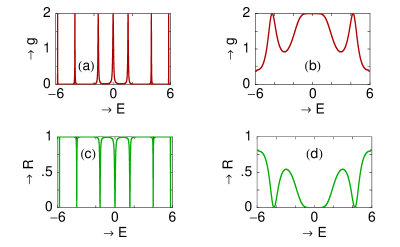
Figure 4: (Color online). Conductance $g$ (red lines) and reflection probability $R$ (green lines) as functions of energy $E$ for two-terminal molecular system. (a) and (c) represent the results for the weak-coupling limit, while (b) and (d) correspond to the same for the strong-coupling limit.

In the weak-coupling regime, the presence of sharp resonant peaks indicates that electron transmission occurs at some typical energy values, while for all other energies conductance vanishes (see Fig. 4(a)). All these resonant peaks are associated with the energy eigenvalues of the molecular system, and therefore, we predict that conductance spectrum is a fingerprint of the electronic structure of the system. Most of the resonant peaks approach the value $2$, the maximum value of $g$ following the Landauer conductance formula (see Eq. 12) and hence $T$ goes to unity at these resonances indicating ballistic transmission through the molecular wire. But the behavior of conductance spectrum changes in case of the strong molecule-to-lead coupling limit. Width of each resonant peak becomes larger and larger as we increase gradually the molecule-to-lead coupling strength and for a large molecular coupling, we have the situation where electron transmission takes place for the entire energy range (for illustration, see Fig. 4(b)). The effect of such broadening comes from the imaginary parts of the self-energies [29]. All these phenomena emphasize that fine tuning in the energy scale is necessary as long as the coupling strength is much weak, while it is not required in case of the strong molecule-to-lead coupling limit.

This scenario is just inverted in case of reflection probability $R$. In the weak-coupling regime, sharp dips appear (Fig. 4(c)) for some particular energy values where conductance shows resonant peaks, as $R$ follows the simple relation $R=1-T$ for the two-terminal molecular system. For all other energy values, $R=1$ indicating no transmission of electron across the molecule. The effect of molecule-to-lead coupling is exactly similar to that for conductance spectrum. In the strong-coupling regime (see Fig. 4(d)), the reflection probability no longer reach the maximum value ($1$) for the entire energy range.

3.1.2 Three-terminal conductance

To illustrate the results for the three-terminal quantum system, constructed by attaching three leads to the molecule (see Fig. 2), let us start by referring to Fig. 5 where the first column shows the conductance spectra $g_{pq}$ (from lead-p to lead-q) and the second column presents the nature of reflection probability $R_{pp}$. Similar to the two-terminal molecular system, some sharp peaks appear in the conductance spectra. But the point is that for the three-terminal system most of the resonant peaks do not reach the value $2$. From the conductance spectra it is clear that the heights are much reduced compared to the two-terminal case. This is solely due to the effect of quantum

Figure 5: (Color online). Conductance $g_{pq}$ (red curves) and reflection probability $R_{pp}$ (green curves) as functions of energy $E$ for three-terminal molecular system. All the results are presented only for the weak-coupling regime.

interference of the electronic waves passing through different arms of the molecular rings. In this three-terminal system, three leads are attached asymmetrically to the molecule at three different locations, which provide different path ways for electron transmission between the leads. This introduces anomalous features in the conductance spectra as illustrated in Figs. 5(a), (b) and (c). More over, in this three-terminal case, nature of variations of reflection probabilities is not so simple as we get in the case of two-terminal molecular system. Here, it is not necessary that $R_{pp}$ shows dips or peaks where $g_{pq}$ has peaks or dips since it ($R_{pp}$) depends on the combined effect of $T_{pq}$’s obeying the expression given in Eq. 9. Another important point we like to mention here is that, one can easily find $T_{qp}$ for any two leads $q$ and $p$ if $T_{pq}$ is known since the relation $T_{pq}=T_{qp}$ holds true following the time-reversal symmetry. The effect of molecule-to-lead coupling strength is identical to the case of two-terminal conductance and therefore, we do not show those results further.

3.1.3 Four-terminal conductance

The transport properties of the four-terminal molecular system is also

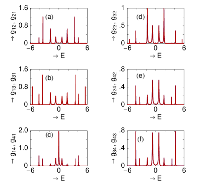
Figure 6: (Color online). Four-terminal conductance $g_{pq}$ as functions of energy $E$ in the limit of weak molecular coupling.

described by investigating various conductances $g_{pq}$ and reflection probabilities $R_{pp}$, which are obtained from the Eqs. 8 and 9, respectively. The results are plotted in Fig. 6 considering the weak molecule-to-lead coupling. In each figure $g_{pq}$ and $g_{qp}$ are plotted and they are superposed to each other due to their symmetry. Sharp resonant peaks of different heights for some particular energies appear in the conductance spectra similar to the two- or three-terminal conductance spectra. From the conductance spectra, the effect of quantum interference associated with the molecule-to-lead interface geometry is well understood.

Figure 7: (Color online). Reflection probability $R_{pp}$ as a function of energy $E$ for four-terminal quantum system. These results correspond to the weak-coupling regime.

Also the dependence of electron transport on molecular coupling strength is exactly similar to that in Fig. 4 and accordingly, the results are not given further. Comparing the results given in Figs. 5 and 6 we observe that, the conductances for two particular leads located at the same positions of the molecule exhibit completely different features in presence of the other leads. For instance, $g_{13}$ of the four-terminal system and $g_{12}$ of the three-terminal system show different spectra though these two conductances are evaluated for the two leads located at the same positions of the molecule. Similarly, careful observation depicts that pathways between the lead-$2$ and lead-$3$ of the three-terminal system are exactly similar to that between lead-$2$ and lead-$4$ of the four-terminal system. In spite of this the corresponding spectra i.e., $g_{23}$ of Fig. 5 and $g_{24}$ of Fig. 6 are different from each other due to the presence of the fourth lead. The effect of the leads are incorporated into the self-energies which lead to the change in conductance spectra. Thus, we can say that the presence of additional leads has a pronounced effect on the electron transport properties. In $R$-$E$ spectra given in Fig. 7, we get various dips at different energies depending on the combined effect of the transmission probabilities (Eq. 9), similar to the case of three-terminal system. All the reflection probabilities are calculated only for the limit of weak molecular coupling. Exactly similar feature, except the broadening, will be observed in the case of strong-coupling.

3.2 Current-voltage characteristics

The scenario of electron transport through molecular junction becomes much more transparent when we discuss the current-voltage ($I$-$V$) characteristics, where the current is evaluated by integrating the transmission probability $T$ using Eq. 13. The nature of the variation of transmission probability is exactly similar to that of conductance spectra except the factor $2$ as we have assumed $e=h=1$ in the Landauer conductance formula (Eq. 12). Here, we discuss the $I$-$V$ characteristics for two-, three- and four-terminal molecular systems separately in the following sub-sections.

3.2.1 Two-terminal molecular system

As an illustration, we display the $I$-$V$ characteristics for the two-terminal system in Fig. 8, where (a) and (b) correspond to the results for the weak and strong molecule-to-lead coupling limits, respectively. For this two-terminal case, current can be expressed mathematically as follows,

$$I = g~{}(V_{1}-V_{2})$$ (14)

$$= g~{}V_{12}$$

where, $V_{12}$ is the voltage difference between the lead-1 and lead-2. In the case of two-terminal molecular system, we have attached two leads to the molecule and their chemical potentials are changed as the bias voltage is applied. With the increase of the voltage, the gap increases more and more and eventually crosses molecular energy levels

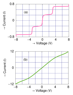
Figure 8: (Color online). Current $I$ as a function of applied bias voltage $V$ for two-terminal molecular system. (a) Weak-coupling limit and (b) strong-coupling limit.

one after another. Accordingly, current channels are opened up and jumps in the $I$-$V$ curve appear. This provides staircase-like structure in the current-voltage spectrum and only for the case of weak molecular coupling these sharp steps appear. But this feature i.e., step-like changes gradually towards continuous nature with the increase of molecule-to-lead coupling strength. In addition to that, current amplitude becomes much higher compared to the case of weak-coupling limit. By noting the area under the curve of Fig. 4(b) the reason behind this enhancement of current amplitude is clearly understood. Thus, it can be manifested that molecule-to-lead coupling strength has a significant influence on molecular transport.

3.2.2 Three-terminal molecular system

Now, we describe the current-voltage characteristics for the three-terminal system where we find the current $I_{p}$ in lead-p by integrating the

Figure 9: (Color online). $I_{1}$ as a function of $V_{13}$ ($=V_{1}-V_{3}$) for the three-terminal molecular system in the limit of strong-coupling, keeping $V_{12}$ ($=V_{1}-V_{2}$) as a constant. The orange, green and magenta colors correspond to $V_{12}=1$, $2$ and $3$, respectively.

transmission function $T_{pq}$ considering the effects of other terminals. To be more precise, we write the current expressions for three different leads as follows,

$$I_{1} = g_{12}\left(V_{1}-V_{2}\right)+g_{13}\left(V_{1}-V_{3}\right)$$ (15)

$$= g_{12}V_{12}+g_{13}V_{13}$$

$$I_{2} = g_{21}\left(V_{2}-V_{1}\right)+g_{23}\left(V_{2}-V_{3}\right)$$ (16)

$$= g_{21}V_{21}+g_{23}V_{23}$$

$$I_{3} = g_{31}\left(V_{3}-V_{1}\right)+g_{32}\left(V_{3}-V_{2}\right)$$ (17)

$$= g_{31}V_{31}+g_{32}V_{32}$$

where, $V_{pq}=\left(V_{p}-V_{q}\right)$ is the voltage difference between the two leads named as lead-p and lead-q.

In Fig. 9, we plot $I_{1}$ for the lead-1 as a function of $V_{13}$ for different fixed values of $V_{12}$ in the strong molecule-to-lead coupling limit. The orange, green and magenta curves represent the currents for $V_{12}=1$, $2$ and $3$, respectively. It is clear from the figure that for a constant value of $V_{12}$, the moment we switch on the bias voltage between lead-1 and lead-3, current rises to a large value. Then, for a wide range of $V_{13}$, it ($I_{1}$) slowly increases with the rise of $V_{13}$ and finally the rate of increment

Figure 10: (Color online). $I_{2}$ as a function of $V_{21}$ ($=V_{2}-V_{1}$) for the three-terminal molecular system in the strong-coupling regime, keeping $V_{23}$ ($=V_{2}-V_{3}$) as a constant. The blue, pink and green lines correspond to $V_{23}=1$, $2$ and $3$, respectively.

of the current gets enhanced when $V_{13}$ is quite high. This behavior i.e., the rate of increment of the current with bias voltage solely depends on the positions of resonant peaks in the $g$-$E$ spectrum. For a particular value of $V_{13}$, $I_{1}$ increases as we increase $V_{12}$ which is clearly visible from three different curves plotted in Fig. 9.

The variation of current $I_{2}$ through lead-2 as a function of $V_{21}$ is shown in Fig. 10, keeping the voltage $V_{23}$ as a constant. The currents are evaluated in the strong-coupling limit, where the blue, pink and green lines correspond to $V_{23}=1$, $2$ and $3$, respectively.

In a similar fashion in Fig. 11 we display $I_{3}$-$V_{31}$ characteristics for different fixed values of $V_{32}$ considering the case of strong-coupling limit. The magenta, green and orange curves correspond to $V_{32}=1$, $3$ and $5$, respectively.

The characteristic features of the currents $I_{1}$, $I_{2}$ and $I_{3}$ passing through three different leads are quite analogous to each other. Depending on the conductance-energy spectra, we get different current amplitudes for three different leads which are clearly observed from the results presented in Figs. 9, 10 and 11. All these currents

Figure 11: (Color online). $I_{3}$ as a function of $V_{31}$ ($=V_{3}-V_{1}$) for the three-terminal molecular system in the strong molecule-to-lead coupling limit, keeping $V_{32}$ as a constant. The magenta, green and orange colors correspond to $V_{32}=1$, $3$ and $5$, respectively.

are computed only for the strong-coupling limit. We can also determine the currents for the limit of weak-coupling and in that case we will get sharp step-like features as a function of bias voltage with much reduced amplitude compared to the strong-coupling case. The origin of step-like behavior in current is clearly mentioned in the case of two-terminal molecular system (Sec. 3.2.1).

From the above current expressions (Eqs. 15, 16 and 17) we see that the current in anyone lead is related to two potential functions. For instance in Eq. 15, there are two parameters like $V_{12}$ and $V_{13}$. Keeping $V_{12}$ as a constant we plot the current $I_{1}$ in terms of $V_{13}$ (see Fig. 9). At the same time, we can also draw the $I_{1}$-$V_{12}$ characteristics, considering $V_{13}$ as a constant. Both for these two cases, the characteristic features are quite similar. This argument is also valid for the other two current expressions (Eqs. 16 and 17).

All the above features of current-voltage characteristics in this three-terminal molecular system clearly support the basic features of a traditional macroscopic transistor. Thus we can predict that the three-terminal molecular system may be utilized to design a nano-scale molecular transistor.

3.2.3 Four-terminal molecular system

Finally, we focus our attention on the current-voltage characteristics for

Figure 12: (Color online). $I_{1}$ as a function of $V_{13}$ for the four-terminal molecular system in the strong-coupling limit, keeping $V_{12}$ and $V_{14}$ as constant. The magenta, green and orange colors correspond to $V_{12}=V_{14}=1$, $3$ and $5$, respectively.

the four-terminal molecular system. In this molecular system, the current expressions for the four different leads are as follows,

$$I_{1} = g_{12}\left(V_{1}-V_{2}\right)+g_{13}\left(V_{1}-V_{3}\right)+g_{14}\left(V_{1}-V_{4}\right)$$ (18)

$$= g_{12}V_{12}+g_{13}V_{13}+g_{14}V_{14}$$

$$I_{2} = g_{21}\left(V_{2}-V_{1}\right)+g_{23}\left(V_{2}-V_{3}\right)+g_{24}\left(V_{2}-V_{4}\right)$$ (19)

$$= g_{21}V_{21}+g_{23}V_{23}+g_{24}V_{24}$$

$$I_{3} = g_{31}\left(V_{3}-V_{1}\right)+g_{32}\left(V_{3}-V_{2}\right)+g_{34}\left(V_{3}-V_{4}\right)$$ (20)

$$= g_{31}V_{31}+g_{32}V_{32}+g_{34}V_{34}$$

$$I_{4} = g_{41}\left(V_{4}-V_{1}\right)+g_{42}\left(V_{4}-V_{2}\right)+g_{43}\left(V_{4}-V_{3}\right)$$ (21)

$$= g_{41}V_{41}+g_{42}V_{42}+g_{43}V_{43}$$

where, $V_{pq}$ is the voltage difference between the lead-p and lead-q.

As representative examples, in Fig. 12 we plot the current in lead-1 ($I_{1}$) as a function of $V_{13}$ keeping $V_{12}$ and $V_{14}$ as constant. The results are computed for the strong-coupling limit, where

Figure 13: (Color online). $I_{2}$ as a function of $V_{24}$ ($=V_{2}-V_{4}$) for the four-terminal molecular system in the limit of strong-coupling, keeping $V_{21}$ and $V_{23}$ as constant. The green, pink and dark-blue lines correspond to $V_{21}=V_{23}=2$, $4$ and $6$, respectively.

the magenta, green and orange curves correspond to $V_{12}=V_{14}=1$, $3$ and $5$, respectively. The variation of current $I_{1}$ as a function of $V_{13}$ in this four-terminal molecular system is quite similar to that as presented in

Figure 14: (Color online). $I_{3}$ as a function of $V_{31}$ for the four-terminal molecular system for the case of strong-coupling limit, considering $V_{32}$ and $V_{34}$ as constant. The green, magenta and dark-blue curves correspond to $V_{32}=V_{34}=1$, $3$ and $5$, respectively.

the case of three-terminal system (Fig. 9). For a particular value of $V_{13}$, here also the current amplitude gets increased with the rise of $V_{12}$ and $V_{14}$. But quite significantly we observe that, for a particular value of $V_{13}$, the current $I_{1}$ passing through the lead-1 of four-terminal system acquires much higher amplitude compared to the three-terminal system (see Figs. 9 and 12). The reason behind this enhancement of current amplitude is explained as follows. From Eq. 18 we see that $I_{1}$ contains three additive terms where the contributions come from other leads, while in Eq. 15 there are two additive terms. The additional term appears in Eq. 18 is due to the presence of fourth terminal which is responsible for the larger current in four-terminal system compared to the three-terminal one.

In case of the current $I_{2}$ through lead-2 we show the variation with respect to $V_{24}$, keeping $V_{21}$ and $V_{23}$ fixed to a particular

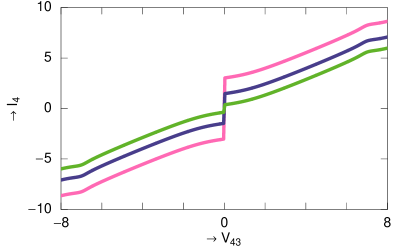
Figure 15: (Color online). $I_{4}$ as a function of $V_{43}$ ($=V_{4}-V_{3}$) for the four-terminal molecular system, keeping $V_{41}$ and $V_{42}$ as constant. The currents are evaluated in the strong-coupling limit, where the green, dark-blue and pink lines correspond to $V_{41}=V_{42}=1$, $5$ and $9$, respectively.

value as presented in Fig. 13. The currents are determined in the strong-coupling regime, where the green, pink and dark-blue lines correspond to $V_{21}=V_{23}=2$, $4$ and $6$, respectively.

Similarly, in Fig. 14 we display $I_{3}$-$V_{31}$ characteristics considering $V_{32}$ and $V_{34}$ as constants in the limit of strong-coupling. The green, magenta and dark-blue lines represent the currents for $V_{32}=V_{34}=1$, $3$ and $5$, respectively.

At the end, in Fig. 15 we show the variation of current $I_{4}$ passing through lead-4 as a function of $V_{43}$ in the limit of strong molecular coupling, when $V_{41}$ and $V_{42}$ are kept as constants. The green, dark-blue and pink curves correspond to the currents for $V_{41}=V_{42}=1$, $5$ and $9$, respectively.

Similar to the case of three-terminal molecular system, for this four-terminal case, we can also plot the current through any lead-p in aspect of the other potential functions as given in Eqs. 18, 19, 20 and 21. For all these cases, the characteristic features are very much similar those are presented in Figs. 12, 13, 14 and 15, and hence, we do not re-plot the results further.

4 Closing remarks

In the present paper we have used a parametric approach to study multi-terminal electron transport through a single phenalenyl molecule. Using a simple tight-binding framework we have performed all the numerical calculations through single particle Green’s function formalism. The basic features of electron transport in this molecular system are explored by investigating the multi-terminal conductance, reflection probability and current. Following a detailed description of electron transport in two-terminal quantum system, we have revealed the essential features of electron transport in the three- and four-terminal quantum systems separately.

Our clear investigation predicts that the electron transport in multi-terminal molecular system significantly depends on (a) the molecule-lead interface geometry, (b) the presence of other leads and (c) the strength of molecular coupling to the side attached leads. The unique characteristics of this phenalenyl molecule with a very small size has enhanced the importance of the present article. Our parametric study provides several significant features to reveal electron transport through any complicated multi-terminal quantum system.

In the present paper we have done all the calculations by ignoring the effects of temperature, electron-electron correlation, etc. We need further study by incorporating all these effects.

References

- [1] N. J. Tao, Nature Nanotechnology 1, 173 (2006).
- [2] A. Aviram and M. Ratner, Chem. Phys. Lett. 29, 277 (1974).
- [3] M. B. Nardelli, Phys. Rev. B 60, 7828 (1999).
- [4] T. Dadosh, Y. Gordin, R. Krahne, I. Khivrich, D. Mahalu, V. Frydman, J. Sperling, A. Yacoby and J. Bar-Joseph, Nature 436, 677 (2005).
- [5] M. A. Reed, C. Zhou, C. J. Muller, T. P. Burgin and J. M. Tour, Science 278, 252 (1997).
- [6] Y. Xue, S. Datta and M. A. Ratner, Chem. Phys. 281, 151 (2002).
- [7] R. Baer and D. Neuhauser, Chem. Phys. 281, 353 (2002).
- [8] R. Baer and D. Neuhauser, J. Am. Chem. Soc. 124, 4200 (2002).
- [9] D. Walter, D. Neuhauser and R. Baer, Chem. Phys. 299, 139 (2004).
- [10] K. Walczak, Cent. Eur. J. Chem. 2, 524 (2004).
- [11] K. Walczak, Phys. Stat. Sol. (b) 241, 2555 (2004).
- [12] M. Büttiker, Phys. Rev. Lett. 57, 1761 (1986).
- [13] H. Q. Xu, App. Phys. Lett. 78, 2064 (2001).
- [14] C. A. Stafford, D. M. Cadamone and S. Mazumdar, Nanotechnology 18, 424014 (2007).
- [15] Q. Sun, B. Wang, J. Wang and T. Lin, Phys. Rev. B 61, 4754 (2000).
- [16] H. K. Zhao, Phys. Lett. A 226, 105 (1997).
- [17] E. G. Emberly and G. Kirczenow, Phys. Rev. B 62, 10451 (2000).
- [18] P. S. Damle, A. W. Ghosh and S. Datta, Phys. Rev. B 64, R201403 (2001).
- [19] P. A. Derosa and J. M. Seminario, J. Phys. Chem. B 105, 471 (2001).
- [20] J. Taylor, H. Guo and J. Wang, Phys. Rev. B 63, 245407 (2001).
- [21] Y. Xue, S. Datta and M. A. Ratner, J. Chem. Phys. 115, 4292 (2001).
- [22] K. Tagami, M. Tsukada, Y. Wada, T. Iwasaki and H. Nishide, J. Chem. Phys. 119, 7491 (2003).
- [23] K. Tagami, L. Wang and M. Tsudaka, Nano Lett. 4, 209 (2004).
- [24] L. Wang, K. Tagami and M. Tsukada, Jpn. J. Appl. Phys. 43, 2779 (2004).
- [25] S. K. Maiti, Phys. Lett. A 373, 4470 (2009).
- [26] S. K. Maiti, J. Phys. Soc. Jpn. 78, 114602 (2009).
- [27] P. O. Lowdin, J. Mol. Spectrosc. 10, 12 (1963).
- [28] P. O. Lowdin, J. Math. Phys. 3, 969 (1962).
- [29] S. Datta, Electronic Transport in Mesoscopic Systems, Cambridge University Press, Cambridge (1997).
- [30] S. Datta, Quantum Transport: Atom to Transistor, Cambridge University Press, Cambridge (2005).
- [31] H. Q. Xu, Phys Rev. B 66, 165305 (2002).
- [32] V. Mujica, M. Kemp and M. A. Ratner, J. Chem. Phys. 101, 6849 (1994).
- [33] S. K. Maiti, Physica E 40, 2730 (2008).
- [34] A. W. Holleitner, R. H. Blick, A. K. Hüttel, K. Eberl and J. P. Kotthaus, Science 297, 70 (2002).