Lattice actions on the plane revisited

Abstract.

We study the action of a lattice $\Gamma$ in the group $G=\operatorname{SL}(2,{\bf R})$ on the plane. We obtain a formula which simultaneously describes visits of an orbit $\Gamma{\mathbf{u}}$ to either a fixed ball, or an expanding or contracting family of annuli. We also discuss the ‘shrinking target problem’. Our results are valid for an explicitly described set of initial points: all ${\mathbf{u}}\in{\bf R}^{2}$ in the case of a cocompact lattice, and all ${\mathbf{u}}$ satisfying certain diophantine conditions in case $\Gamma=\operatorname{SL}(2,{\mathbb{Z}})$. The proofs combine the method of Ledrappier with effective equidistribution results for the horocycle flow on $\Gamma\backslash G$ due to Burger, Strömbergsson, Forni and Flaminio.

1. Introduction, statement of the results

A classical problem in ergodic theory is to understand the distribution of orbits for the action of a group on a space. This has been particularly well-studied under the hypotheses that the acting group $\Gamma$ is amenable and preserves a finite measure. Removing these two assumptions leads to a realm which is not sufficiently understood. Our purpose in this note is to describe some features which arise when one studies a non-amenable group acting on a space preserving an infinite Radon measure. We will consider the simplest setup with these features. Namely, let $\Gamma$ be a lattice in $G=\operatorname{SL}(2,{\bf R})$, that is, a discrete subgroup of finite covolume. It acts on the punctured plane $\mathcal{P}={\bf R}^{2}\smallsetminus\{0\}$ by linear transformations, preserving Lebesgue measure. It is well-known that this action is ergodic. Moreover, when $\Gamma$ is cocompact all orbits are dense, and when $\Gamma$ is non-uniform, any orbit is either discrete or dense.

Consider an orbit $\Gamma{\mathbf{u}}$ and an increasing family $\{\Gamma_{T}:T>0\}$ of finite sets in $\Gamma$. We will refer to $\Gamma_{T}{\mathbf{u}}\subset\mathcal{P}$ as a ‘cloud’; we wish to understand its distribution for large values of $T$. For example one can ask for the frequency of visits to a fixed ball in the plane. One can also consider the behavior of the orbit under rescaling, i.e. the frequency of visits to a family of balls; if the balls are expanding with $T$ this corresponds to the ‘large scale’ behavior of the orbit and if the balls are shrinking this corresponds to the behavior of the orbit ‘at a point.’ The answers to these questions turn out to depend rather delicately on the choice of the averaging sets $\Gamma_{T}$ and the initial point ${\mathbf{u}}$.

Fix a norm $\|\cdot\|$ on ${\operatorname{M}}_{2}({\bf R})$, the space of two by two matrices with real entries. Define for any $T>0$ the set

$$\Gamma_{T}=\left\{\gamma\in\Gamma\,:\,\|\gamma\|\leq T\right\},$$

let $f$ be a compactly supported function on $\mathcal{P}$ and ${\mathbf{u}}\in{\bf R}^{2}$.

Figure 1. ‘Cloud’ for the cocompact lattice $\operatorname{SL}_{1}(D_{2,3}({\bf Z})),\,{\mathbf{u}}=(1,0),\,T=100.$

The asymptotics of the orbit-sum

$$S_{f,{\mathbf{u}}}(T)=\sum_{\gamma\in\Gamma_{T}}f(\gamma{\mathbf{u}})$$

were studied in [L, N, GW]. Write ${\mathbf{u}}=\left[\begin{array}[]{c}u_{1}\\ u_{2}\end{array}\right]\in{\bf R}^{2}$, and define a norm $|\cdot|$ and a ‘product’ $\star$ on ${\bf R}^{2}$ by

$$|{\mathbf{v}}|=\max\left\{|v_{1}|,|v_{2}|\right\},\ \ \ {\mathbf{v}}\star{\mathbf{u}}=\Biggl{\|}\left[\begin{array}[]{cc}-u_{2}v_{1}&u_{1}v_{1}\\ -u_{2}v_{2}&u_{1}v_{2}\\ \end{array}\right]\Biggr{\|},$$

where ${\mathbf{v}}=\left[\begin{array}[]{c}v_{1}\\ v_{2}\end{array}\right]$. Let $dx$ denote the Lebesgue measure on $\mathcal{P}$. It was shown in the above-mentioned papers (see particularly [GW, §12.4]) that

$$\frac{S_{f,{\mathbf{u}}}(T)}{T}\ \longrightarrow_{T\to\infty}\ \frac{2}{\mu(\Gamma\backslash G)}\int_{\mathcal{P}}\frac{f({\mathbf{v}})}{{\mathbf{v}}\star{\mathbf{u}}}\,d{\mathbf{v}}.$$

We would like to understand $S_{f,{\mathbf{u}}}(T)$ at a finite time $T$, i.e. obtain an effective error estimate in this asymptotic formula. In particular we would like to be able to change the function $f$ and the initial point ${\mathbf{u}}$ depending on the time $T$. Before stating our results we introduce some notation.

Write ${\rm supp}\,f=\overline{f^{-1}({\bf R}\smallsetminus\{0\})}$, and set

$$\begin{split}r(f)&=\inf_{{\mathbf{v}}\in{\rm supp}\,f}|{\mathbf{v}}|,\ \ \ \ \ \ \ R(f)=\sup_{{\mathbf{v}}\in{\rm supp}\,f}|{\mathbf{v}}|,\ \ \ \ \ v(f)=\frac{R(f)}{r(f)}.\end{split}$$

The homogeneous space $\Gamma\backslash G$ carries a finite measure $\mu$ invariant under the right action of $G$; we will normalize this measure by assuming that its lift to $G$ satisfies (2.9). Fix $\theta\in(0,1]$. We say that a continuous compactly supported function $f$ on $\mathcal{P}$ is $\theta$-Hölder if $\|f\|_{\theta}<\infty$, where

(1.1) $${\|f\|_{\theta}=\sup|f|+\left(\int_{\mathcal{P}}f({\mathbf{v}})^{2}\frac{d{\mathbf{v}}}{|{\mathbf{v}}|^{2}}\right)^{1/2}+\sup_{0<|x-y|\leq|x|/2}\frac{|x|^{\theta}|f(x)-f(y)|}{|x-y|^{\theta}}.}$$

Theorem 1.1.

For a cocompact lattice $\Gamma$ in $G$ there are positive constants $c$ and $\delta_{0}$ such that for any $\theta\in(0,1]$, there is a positive constant $C_{\theta}$ such that the following holds. For any ${\mathbf{u}}\in\mathcal{P}$ and for any $\theta$-Hölder $f:\mathcal{P}\to{\bf R}$, of compact support, let

(1.2) $${D_{0}=D_{0}({\mathbf{u}},f)=\max\left(\frac{R(f)}{|{\mathbf{u}}|},\frac{|{\mathbf{u}}|}{r(f)}\right)}$$

and

(1.3) $${B=B({\mathbf{u}},f)=\left(\frac{R(f)}{|{\mathbf{u}}|}\right)^{-\theta\delta_{0}}(\log v(f)+1).}$$

Then for any

(1.4) $${T>T_{0}=cD_{0}}$$

one has

(1.5) $${\left|S_{f,{\mathbf{u}}}(T)-\frac{2T}{\mu(\Gamma\backslash G)}\int_{\mathcal{P}}\frac{f({\mathbf{v}})}{{\mathbf{v}}\star{\mathbf{u}}}\,d{\mathbf{v}}\right|\leq C_{\theta}\|f\|_{\theta}\frac{R(f)}{|{\mathbf{u}}|}\left(D_{0}+BT^{1-\theta\delta_{0}}\right).}$$

Remark 1.2.

1. Our proof shows one may take $\delta_{0}=\delta_{\Gamma}/21$, where $\delta_{\Gamma}\leq 1/2$ satisfies $\delta_{\Gamma}(\delta_{\Gamma}-1)\leq\lambda,$ with $\lambda<0$ the first eigenvalue of the Laplacian on $\Gamma\backslash G$. Our exponent is not optimal.

2. The inequality (1.5) behaves as should be expected under rescaling. More precisely, for any $\lambda>0$, if one replaces $f({\mathbf{v}})$ by $g({\mathbf{v}})=f(\lambda{\mathbf{v}})$, and ${\mathbf{u}}$ by ${\mathbf{w}}=\lambda^{-1}{\mathbf{u}}$, then $D_{0}({\mathbf{u}},f)=D_{0}({\mathbf{w}},g)$, $B({\mathbf{u}},f)=B({\mathbf{w}},g)$, $T_{0}$ does not change either, and both sides of (1.5) are unaffected.

The explicit error term in Theorem 1.1 is useful for studying the asymptotic behavior of an orbit under rescaling. For an ‘expansion coefficient’ $\rho>0$ consider the function $\displaystyle{f_{\rho}(x)=f\left(\frac{x}{\rho}\right)}.$ Then for a parameter $\alpha$, $f_{T^{\alpha}}$ describes a one-parameter family of functions, and we are interested in sampling them with the cloud $\Gamma_{T}{\mathbf{u}}$. For instance, if $f$ is the indicator function of an annulus of radius 1 then the orbit-sum $S_{f_{T^{\alpha}},{\mathbf{u}}}(T)$ describes the number of orbit points in the cloud contained in the similar annulus of radius $T^{\alpha}$. Since the diameter of the cloud is approximately $T$, if $\alpha>1$ the orbit-sum will vanish for large $T$, and similarly for $\alpha<-1$. However as long as the expansion of the cloud is faster than that of the support of the expanded function, the cloud equidistributes in the support of the function, with respect to the same asymptotic density as in Theorem 1.1. Namely we have:

Corollary 1.3.

Given a cocompact lattice $\Gamma$ in $G$ and $-1<\alpha<1$, $0<\theta\leq 1$, there is $\delta>0$ such that for any ${\mathbf{u}}\in\mathcal{P}$ and any compactly supported $\theta$-Hölder function $f$ on $\mathcal{P}$ there are positive $T_{0}$ and $C$ such that for all $T>T_{0}$,

(1.6) $${\left|\frac{1}{T^{1+\alpha}}\sum_{\gamma\in\Gamma_{T}}f\left(\frac{\gamma{\mathbf{u}}}{T^{\alpha}}\right)-\frac{2}{\mu(\Gamma\backslash G)}\int_{\mathcal{P}}\frac{f({\mathbf{v}})}{{\mathbf{v}}\star{\mathbf{u}}}\,d{\mathbf{v}}\right|<CT^{-\delta}.}$$

Remark 1.4.

1. Adapting the arguments used in the proof of Corollary 1.3 one can show that for any continuous compactly supported function $\phi$ on $\mathcal{P}$ for which $\displaystyle{\frac{\phi(T)}{T}\to 0}$ and $T\phi(T)\to\infty$, one has

   $$\ \frac{S_{f_{\phi(T)},{\mathbf{u}}}}{T\phi(T)}\to\frac{2}{\mu\left(\Gamma\backslash G\right)}\int_{\mathcal{P}}\frac{f({\mathbf{v}})}{{\mathbf{v}}\star{\mathbf{u}}}\,d{\mathbf{v}}.$$

2. The case $\alpha=1$, that is the asymptotic behavior of $\frac{1}{T^{2}}S_{f_{T},{\mathbf{u}}}$ was studied in [M]. In this case the asymptotic density is different.

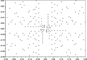
(a) $T=100$

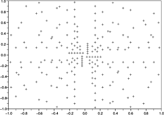
(b) $T=25$

(c) $T=9$

Figure 2. The ‘scaling property’. For $\Gamma=\operatorname{SL}(2,{\bf Z})$, parts of the orbit of three different points are shown, at different scales and with different values of $T$. Each contains approximately 200 points.

Theorem 1.1 does not hold in the non-uniform case. For example, there are discrete orbits for $\Gamma$ in the plane, and these certainly will not satisfy (1.5) if ${\rm supp}f$ does not intersect the orbit; consequently, for a fixed $T$ the conclusion of Corollary 1.3 will also fail for all ${\mathbf{u}}$ sufficiently close to a point with a discrete orbit. The behavior of the orbit will depend in a subtle way on the diophantine properties of the slope of the initial vector; to make this precise, we will need a bit of notation.

Let $z\in[0,1)$, and denote $z=[0;a_{1},a_{2},\ldots]$ its continued fraction expansion, $p_{k},q_{k}$ its convergents. Let $t_{k}=-\log\left|z-\frac{p_{k}}{q_{k}}\right|$; the theory of continued fractions (see [HW]) tells us that $(t_{k})_{k}$ is an increasing sequence, and that

(1.7) $${a_{k+1}q_{k}^{2}\leq e^{t_{k}}\leq(a_{k+1}+2)q_{k}^{2}.}$$

Define, in the case where $z$ is irrational

$$\hat{\xi}(z,\tau_{1},\tau_{2})=\max\left(a_{k}\,:\,\tau_{1}\leq t_{k+1},\,t_{k-1}\leq\tau_{2}\right)$$

(if the set on the right hand side is empty we set $\hat{\xi}(z,\tau_{1},\tau_{2})=e^{\tau_{2}}$). If $z$ is rational, the sequences $(a_{k})$, $(q_{k})$ and $(t_{k})$ are finite. Let $k_{0}$ be the length, that is $z=p_{k_{0}}/q_{k_{0}}$. If $\tau_{2}\leq t_{k_{0}-1}$, $\hat{\xi}(z,\tau_{1},\tau_{2})$ is defined by the preceding formula; if not,

$$\hat{\xi}(z,\tau_{1},\tau_{2})=\min\left(e^{\tau_{2}},\max\left(\max\{a_{k}\,:\,\tau_{1}\leq t_{k+1}\},e^{\tau_{2}}/q_{k_{0}}^{2}\right)\right).$$

If ${\mathbf{u}}=\left[\begin{array}[]{c}{\mathbf{u}}_{x}\\ {\mathbf{u}}_{y}\end{array}\right]\in\mathcal{P}$, denote by $z$ the unique real number in the set $[0,1]\cap\{{\mathbf{u}}_{x}/{\mathbf{u}}_{y},{\mathbf{u}}_{x}/{\mathbf{u}}_{y}+1,-{\mathbf{u}}_{y}/{\mathbf{u}}_{x},-{\mathbf{u}}_{y}/{\mathbf{u}}_{x}+1\}$. We define $\hat{\xi}({\mathbf{u}},\tau_{1},\tau_{2})=\hat{\xi}(z,\tau_{1},\tau_{2})$.

Theorem 1.5.

For $\Gamma=\operatorname{SL}(2,{\bf Z})$ there are positive constants $c$ and $\delta_{0}$ such that for any $\theta\in(0,1]$, there exists $C>0$ such that the following holds. For any ${\mathbf{u}}\in\mathcal{P}$ and for any compactly supported $\theta$-Hölder map $f:\mathcal{P}\to{\bf R}$, let $D_{0}$ and $B$ be as in (1.2) and (1.3), and let

$$\hat{\xi}_{f,T,{\mathbf{u}}}=\hat{\xi}\left({\mathbf{u}},\log\left(\frac{T|{\mathbf{u}}|}{R(f)}\right),\log\left(\frac{T|{\mathbf{u}}|}{r(f)}\right)\right).$$

Then for any $T>cD_{0}$ such that

(1.8) $${T\geq c\ \frac{|{\mathbf{u}}|\hat{\xi}_{f,T,{\mathbf{u}}}}{R(f)}}$$

one has

(1.9) $${\left|S_{f,{\mathbf{u}}}(T)-\frac{2T}{\mu(\Gamma\backslash G)}\int_{\mathcal{P}}\frac{f({\mathbf{v}})}{{\mathbf{v}}\star{\mathbf{u}}}\,d{\mathbf{v}}\right|\leq C\|f\|_{\theta}\frac{R(f)}{|{\mathbf{u}}|}\left(D_{0}+BT^{1-\theta\delta_{0}}\hat{\xi}_{f,T,{\mathbf{u}}}^{\theta\delta_{0}}\right).}$$

Remark 1.6.

1. Examining our argument one sees it is possible to take $\delta_{0}=1/48$ in Theorem 1.5.

2. Our arguments prove an analogous result for any lattice $\Gamma$ in place of $\operatorname{SL}(2,{\bf Z})$. In this case, the quantity $\hat{\xi}({\mathbf{u}},\tau_{1},\tau_{2})$ is replaced by the supremum of the distance between a fixed reference point in $\Gamma\backslash G$ and $\Psi({\mathbf{u}}/|{\mathbf{u}}|)a_{s}$, where $s\in[\tau_{1},\tau_{2}]$ — see §§7-8. Also, the $\delta_{0}$ can be taken to be $\delta_{\Gamma}/24$, where $\delta_{\Gamma}$ is defined as explained in Remark 1.4(1).

For $\beta>0$, say $z\in{\bf R}$ is $\beta$-diophantine if there is $c>0$ such that $|z-p/q|\geq cq^{-\beta}$ for all $p,q\in{\bf Z}$. Note that quadratic irrationals are $2$-diophantine, and by Roth’s theorem, all algebraic numbers are $2+\varepsilon$-diophantine for any $\varepsilon>0$, like Lebesgue almost any real number. In the following, we extend the definition to the case $\beta=+\infty$ with the convention that every number (even rationals) is $\infty$-diophantine. It is well-known (see Lemma 7.2) that when $z$ is $\beta$-diophantine, $\hat{\xi}_{z,\tau_{1},\tau_{2}}$ can be bounded in terms of $\beta$. This yields:

Corollary 1.7.

Given $\beta\in[2,+\infty]$, $\theta\in(0,1]$ and $-\frac{1}{\beta-1}<\alpha<1$, there is $\delta>0$ such that for any ${\mathbf{u}}\in\mathcal{P}$ a vector with a $\beta$-diophantine slope and any compactly supported $\theta$-Hölder function $f$ on $\mathcal{P}$ there are positive $T_{0}$ and $C$ such that for all $T>T_{0}$,

(1.10) $${\left|\frac{1}{T^{1+\alpha}}\sum_{\gamma\in\Gamma_{T}}f\left(\frac{\gamma{\mathbf{u}}}{T^{\alpha}}\right)-\frac{2}{\mu(\Gamma\backslash G)}\int_{\mathcal{P}}\frac{f({\mathbf{v}})}{{\mathbf{v}}\star{\mathbf{u}}}\,d{\mathbf{v}}\right|<CT^{-\delta}.}$$

Remark 1.8.

In a recent and independent work [N2], Nogueira proved a similar result, with a better estimate of the error term, but in the particular case in which $f$ is the characteristic function of a square, and the norm $||\cdot||$ is the supremum norm, generalizing his previous results [N]. The method used is completly different from ours.

Applying Theorem 1.5 to the ‘shrinking target problem’, we obtain:

Corollary 1.9.

Let $\delta_{0}$ be as in Theorem 1.5, and let ${\mathbf{v}},{\mathbf{u}}\in\mathcal{P}$. Then:

1. If ${\mathbf{u}}$ has $\beta$-diophantine slope, then there are positive constants $C$ and $T_{0}$ such that for all $T\geq T_{0}$ there is $\gamma\in\Gamma_{T}$ such that

   $$|\gamma{\mathbf{u}}-{\mathbf{v}}|<CT^{-\frac{2\delta_{0}}{3\beta}}.$$

2. If the slope of ${\mathbf{u}}$ is irrational then there is a positive constant $C$ such that there are infinitely many $\gamma\in\Gamma$ solving

   $$|\gamma{\mathbf{u}}-{\mathbf{v}}|<C||\gamma||^{-\frac{\delta_{0}}{3}}.$$

1.1. Notation

Throughout this paper the Vinogradov symbol $A\ll B$ means that there is a constant $C$ such that $A\leq CB$, where $A$ and $B$ are expressions depending on various quantities and the implicit constant $C$ is independent of these quantities. In particular, throughout the paper the implicit constant may depend on $\Gamma$, on the choice of the norm $\|\cdot\|$, on auxilliary functions $\Psi,\,\phi$, but not on the function $f$ nor the initial point ${\mathbf{u}}$. The notation $A\asymp B$ means that $A\ll B$ and $B\ll A$.

2. The norm estimate

2.1. The setup

Let $G$ act on ${\bf R}^{2}$ by matrix multiplication on the left. Define the following matrices

$$h_{s}=\left[\begin{array}[]{cc}1&s\\ 0&1\\ \end{array}\right],\;a_{t}=\left[\begin{array}[]{cc}e^{t/2}&0\\ 0&e^{-t/2}\\ \end{array}\right],\;r_{\theta}=\left[\begin{array}[]{cc}\cos\theta&-\sin\theta\\ \sin\theta&\cos\theta\\ \end{array}\right].$$

The stabilizer of ${\mathbf{u}}_{0}=\left[\begin{array}[]{c}1\\ 0\end{array}\right]$ is precisely the unipotent subgroup

$$H=\{h_{s}\,:\,s\in{\bf R}\},$$

so that $\mathcal{P}$ is identified with the quotient $G/H$ via the map $gH\mapsto g{\mathbf{u}}_{0}$. Let $\Gamma$ be a lattice in $G$, and let $\tau:G\to G/H$ and $\pi:G\to\Gamma\backslash G$ be the natural quotient maps.

We define a haar measure $\lambda$ on $H$ by $d\lambda(h_{s})=ds$.

2.2. The section

Define $\Psi:\mathcal{P}\rightarrow G$ by

(2.1) $${\Psi\left(\left[\begin{array}[]{c}x\\ y\end{array}\right]\right)=\left[\begin{array}[]{cc}x&-y/(x^{2}+y^{2})\\ y&x/(x^{2}+y^{2})\\ \end{array}\right],}$$

The function $\Psi$ is a section in the sense that $\tau\circ\Psi=\mathrm{Id}|_{G/H}$, i.e. for all ${\mathbf{u}}\in\mathcal{P},$

(2.2) $${\Psi({\mathbf{u}}){\mathbf{u}}_{0}={\mathbf{u}}.}$$

The following equation is easily verified:

(2.3) $${{\mathbf{v}}\star{\mathbf{u}}=\Biggl{\|}\Psi({\mathbf{v}})\left[\begin{array}[]{cc}0&1\\ 0&0\\ \end{array}\right]\Psi({\mathbf{u}})^{-1}\Biggr{\|}.}$$

Note that (2.3) does not depend on the choice of the section $\Psi$ (as might not be obvious from the formula). It can be also checked that for any $t\in{\bf R}$ and ${\mathbf{v}}\in\mathcal{P}$, we have

(2.4) $${\Psi(e^{t}{\mathbf{v}})=\Psi({\mathbf{v}})a_{2t}.}$$

Define

(2.5) $${D=D({\mathbf{u}},f)=\sup_{x\in{\rm supp}\,f}\|\Psi(x)\Psi({\mathbf{u}})^{-1}\|,}$$

this quantity satisfies

(2.6) $${D({\mathbf{u}},f)\asymp D_{0}({\mathbf{u}},f),}$$

where $D_{0}$ is as in (1.2). Indeed, let $x\in{\rm supp}\,f$, then

$$\|\Psi(x)\Psi({\mathbf{u}})^{-1}\|=\left\|\Psi\left(\frac{x}{|x|}\right)a_{2\log(|x|/|{\mathbf{u}}|)}\Psi\left(\frac{{\mathbf{u}}}{|{\mathbf{u}}|}\right)^{-1}\right\|$$

$$\asymp\|a_{2\log(|x|/|{\mathbf{u}}|)}\|\asymp\max\left(\frac{|x|}{|{\mathbf{u}}|},\frac{|{\mathbf{u}}|}{|x|}\right).$$

2.3. The cocycle

Let ${\mathbf{u}}\in\mathcal{P}$ and $g\in G$, define $c_{{\mathbf{u}}}(g)$ by the following implicit equation:

(2.7) $${\left[\begin{array}[]{cc}1&c_{{\mathbf{u}}}(g)\\ 0&1\\ \end{array}\right]=\Psi(g{\mathbf{u}})^{-1}g\Psi({\mathbf{u}}).}$$

This makes sense because the right hand side stabilizes ${\mathbf{u}}_{0}$, so is in $H$. It is easily checked that $c$ is a cocycle, meaning it satisfies for any $g_{1},g_{2}\in G$ and ${\mathbf{u}}\in\mathcal{P}$,

$$c_{{\mathbf{u}}}(g_{1}g_{2})=c_{g_{2}{\mathbf{u}}}(g_{1})+c_{{\mathbf{u}}}(g_{2}).$$

One also sees that in terms of Iwasawa decomposition, we have

(2.8) $${g=kan\ \ \implies\ \ ka=\Psi(g{\mathbf{u}}_{0}),\ n=h_{s}\ \mathrm{where}\ s=c_{{\mathbf{u}}_{0}}(g).}$$

Therefore we can write haar measure $\mu$ on $G$ by the formula

(2.9) $${d\mu(g)=d\tau(g)\,d\lambda(c_{{\mathbf{u}}_{0}}(g)).}$$

Note that the normalization of Lebesgue measure on ${\bf R}^{2}$ and $\lambda$ determine a normalization for $\mu$. Changing the section $\Psi$ gives rise to a homologous cocycle, so that $\mu$ is actually independent of $\Psi$. It follows from (2.8) that

(2.10) $${c_{{\mathbf{u}}_{0}}(gh_{s})=c_{{\mathbf{u}}_{0}}(g)+s,\ \ \ \ c_{{\mathbf{u}}_{0}}(ga_{t})=e^{-t}c_{{\mathbf{u}}_{0}}(g),}$$

and from (2.2) that

(2.11) $${c_{{\mathbf{u}}}(g)=c_{{\mathbf{u}}_{0}}(g\Psi({\mathbf{u}})).}$$

Lemma 2.1.

Let $D=D({\mathbf{u}},f)$ be as in (2.5). For any $f\in C_{c}(\mathcal{P})$, any ${\mathbf{u}}\in\mathcal{P}$ and any $g\in G$ for which $g{\mathbf{u}}\in{\rm supp}\,f$ we have

(2.12) $${\Bigl{|}\|g\|-|c_{{\mathbf{u}}}(g)|\,(g{\mathbf{u}}\star{\mathbf{u}})\Bigr{|}\leq D.}$$

Proof.

By (2.7), we have

$$\begin{split}g&=\Psi(g{\mathbf{u}})\left(\mathrm{Id}+\left[\begin{matrix}0&c_{{\mathbf{u}}}(g)\\ 0&0\end{matrix}\right]\right)\Psi({\mathbf{u}})^{-1}\\ &=\Psi(g{\mathbf{u}})\Psi({\mathbf{u}})^{-1}+c_{{\mathbf{u}}}(g)\Psi(g{\mathbf{u}})\left[\begin{matrix}0&1\\ 0&0\end{matrix}\right]\Psi({\mathbf{u}})^{-1}.\end{split}$$

By (2.3),

$$\left\|c_{{\mathbf{u}}}(g)\Psi(g{\mathbf{u}})\left[\begin{matrix}0&1\\ 0&0\end{matrix}\right]\Psi({\mathbf{u}})^{-1}\right\|=|c_{{\mathbf{u}}}(g)|\,(g{\mathbf{u}}\star{\mathbf{u}}).$$

The claim follows. ∎

2.4. Some useful inequalities

Here we state and prove elementary inequalities that will be useful later. The first remark is that the $\star$-product is well-approximated by the product of the norms:

(2.13) $${{\mathbf{v}}\star{\mathbf{u}}\asymp|{\mathbf{v}}|\,|{\mathbf{u}}|.}$$

Indeed,

$${\mathbf{v}}\star{\mathbf{u}}=\Biggl{\|}\left[\begin{array}[]{cc}-u_{2}v_{1}&u_{1}v_{1}\\ -u_{2}v_{2}&u_{1}v_{2}\\ \end{array}\right]\Biggr{\|}\asymp\max_{i,j=1,2}\{|u_{i}v_{j}|\}=\max_{i=1,2}\{|u_{i}|\}\max_{j=1,2}\{|v_{j}|\}.$$

The following upper bound will also prove helpful: for any $\theta$-Hölder compactly supported $f:\mathcal{P}\to{\mathbb{R}}$

(2.14) $${\left|\int_{\mathcal{P}}\frac{f({\mathbf{v}})}{{\mathbf{v}}\star{\mathbf{u}}}\,d{\mathbf{v}}\right|\ll\|f\|_{\theta}\frac{R(f)}{|{\mathbf{u}}|}.}$$

This is proved as follows:

$$\left|\int_{\mathcal{P}}\frac{f({\mathbf{v}})}{{\mathbf{v}}\star{\mathbf{u}}}\,d{\mathbf{v}}\right|\stackrel{{\scriptstyle\eqref{eq: eq: starproduct}}}{{\ll}}\left|\int_{{\rm supp}\,f}\frac{f({\mathbf{v}})}{|{\mathbf{v}}|\,|{\mathbf{u}}|}\,d{\mathbf{v}}\right|\ll|{\mathbf{u}}|^{-1}\left(\int_{\mathcal{P}}f^{2}({\mathbf{v}})|{\mathbf{v}}|^{-2}\,d{\mathbf{v}}\right)^{1/2}\left(\int_{{\rm supp}\,f}d{\mathbf{v}}\right)^{1/2},$$

by the Cauchy-Schwarz inequality, and since ${\rm supp}\,f$ is in a disk of radius approximately $R(f)$, this implies (2.14).

3. From the plane to the homogeneous space

In this section we pass from a function $f:\mathcal{P}\to{\bf R}$ to a function $\bar{f}:\Gamma\backslash G\to{\bf R}$. This is done in two steps: lifting to a function $\widetilde{f}$ using the section $\Psi$ and a bump function; and summing along $\Gamma$-orbits to obtain a function $\bar{f}$ on $\Gamma\backslash G$.

Assume $f$ is compactly supported and non-negative. Fix $\phi:{\bf R}\rightarrow{\bf R}$ a nonnegative $C^{\infty}$ function, vanishing outside $[-1,1]$, such that $\int_{\bf R}\phi(t)dt=1$. Set

(3.1) $${\widetilde{f}:G\to{\bf R},\ \ \widetilde{f}(g)=f(\tau(g))\phi(c_{{\mathbf{u}}_{0}}(g))}$$

(a compactly supported smooth function on $G$) and

(3.2) $${\bar{f}(x)=\sum_{g\in\pi^{-1}(x)}\widetilde{f}(g)}$$

(a finite sum for each $x$). The normalization (2.9) for $\mu$ ensures that

(3.3) $${\int_{\Gamma\backslash G}\bar{f}\,d\mu=\int_{{\bf R}^{2}}f(x)\,dx.}$$

The distribution of the cloud $\Gamma_{T}$ turns out to be linked with the norm ${\mathbf{v}}\mapsto{\mathbf{v}}\star{\mathbf{u}}$, and for this reason we will have to work with the more precise measures of the support of $f$:

$$r^{({\mathbf{u}})}(f)=\inf_{{\mathbf{v}}\in{\rm supp}\,f}{\mathbf{v}}\star{\mathbf{u}}\asymp r(f)\,|{\mathbf{u}}|,\ \ \ \ \ \ \ R^{({\mathbf{u}})}(f)=\sup_{{\mathbf{v}}\in{\rm supp}\,f}{\mathbf{v}}\star{\mathbf{u}}\asymp R(f)\,|{\mathbf{u}}|,$$

$$v^{({\mathbf{u}})}(f)=\frac{R^{({\mathbf{u}})}(f)}{r^{({\mathbf{u}})}(f)}\asymp v(f).\\$$

Lemma 3.1.

Let ${\mathbf{u}}\in\mathcal{P},\,\widetilde{\mathbf{u}}=\Psi({\mathbf{u}}),\,\gamma\in\Gamma,\,f\in C_{c}(\mathcal{P})$ and let $\widetilde{f}$ be as in (3.1). Let $D=D({\mathbf{u}},f)$ be as in (2.5).

Then

(3.4) $${\begin{split}r\leq r^{({\mathbf{u}})}(f),\ \|\gamma\|\leq T&\ \implies\ \int_{-\left(1+(T+D)/r\right)}^{1+(T+D)/r}\widetilde{f}(\gamma\widetilde{\mathbf{u}}h_{s})\,ds=f(\gamma{\mathbf{u}}),\\ R^{({\mathbf{u}})}(f)\leq R,\ \|\gamma\|\geq T&\ \implies\ \int_{-\left((T-D)/R-1\right)}^{(T-D)/R-1}\widetilde{f}(\gamma\widetilde{\mathbf{u}}h_{s})\,ds=0.\end{split}}$$

Proof.

Since $\int\phi(s)ds=1$ and ${\rm supp}\,\phi\subset[-1,1]$, for the first claim it suffices to show that for $\|\gamma\|\leq T$ and $\gamma{\mathbf{u}}\in{\rm supp}\,f$ we have

$$[-1,1]\subset\left\{c_{{\mathbf{u}}_{0}}(\gamma\widetilde{\mathbf{u}}h_{s}):|s|\leq 1+(T+D)/r\right\},$$

or by (2.10), that

$$|c_{{\mathbf{u}}_{0}}(\gamma\widetilde{\mathbf{u}})|\leq\frac{T+D}{r}.$$

This follows from (2.11) and (2.12). The proof of the second claim is similar. ∎

We will need to control the Hölder norm of $\bar{f}$ in terms of that of $f$. For $\theta\in(0,1]$, define a Hölder norm on compactly supported function $f$ on $G$ or $\Gamma\backslash G$:

$$||f||_{\theta}=\sup_{{\mathrm{dist}}(x,y)\leq 1}\frac{|f(x)-f(y)|}{{\mathrm{dist}}(x,y)^{\theta}}.$$

Here by dist we denote a left-invariant Riemannian metric on $G$, or the corresponding metric induced on $\Gamma\backslash G$.

Lemma 3.2.

For any $\sigma>1$ and any $\theta\in(0,1]$ there is a constant $c=c_{\sigma,\theta}>0$ and a compact set $K_{\sigma}\subset\Gamma\backslash G$ such that for any $\theta$-Hölder compactly supported function $f$ with

$${\rm supp}\,f\subset A_{\sigma}=\{{\mathbf{w}}\in\mathcal{P}\,:\,\sigma^{-1}\leq|{\mathbf{w}}|\leq\sigma\},$$

we have ${\rm supp}\,\bar{f}\subset K_{\sigma}$ and

(3.5) $${\|\bar{f}\|_{\theta}\leq c\|f\|_{\theta}.}$$

Proof.

We first prove that for some constant $c_{1}>0$,

$$\|\widetilde{f}\|_{\theta}\leq c_{1}\|f\|_{\theta}.$$

Note that since $\widetilde{f}(g)=f(\tau(g))\phi(c_{{\mathbf{u}}_{0}}(g))$, the support of $\widetilde{f}$ is contained in the compact set $\widetilde{K}_{\sigma}=\tau^{-1}(A_{\sigma})\cap c_{{\mathbf{u}}_{0}}^{-1}([-1,1])$, and that $\tau$, $\phi\circ c_{{\mathbf{u}}_{0}}$ are Lipschitz when restricted to $K_{\sigma}$, so

$$\|\widetilde{f}\|_{\theta}\ll\|f\|_{\theta}.$$

Also note that $\#\,\widetilde{K}_{\sigma}\cap\pi^{-1}(x)$ is bounded independently of $x$ by compactness of $\widetilde{K}_{\sigma}$, by a bound depending on $\sigma$ only. Thus,

$$\|\bar{f}\|_{\theta}\ll\|\widetilde{f}\|_{\theta}.$$

We put $K_{\sigma}=\pi(\widetilde{K}_{\sigma})$. ∎

4. Radial Partition of unity

We will use a partition of unity to reduce to the case when ${\rm supp}\,f$ is contained in a narrow annulus around zero. Let $\kappa$ be the ‘tent’ map

$$\kappa(x)=\begin{cases}0&\text{if $x\leq-1$ or $x\geq 1$},\\ x+1&\text{if}\ -1\leq x\leq 0,\\ 1-x&\text{if}\ 0\leq x\leq 1,\\ \end{cases}$$

which is a $1$-Lipschitz map and satisfies for all $x$

(4.1) $${\sum_{\ell\in{\mathbb{Z}}}\kappa(x+\ell)=1.}$$

Now given a parameter $\alpha\geq 1$, for any Hölder function $f$ on $\mathcal{P}$ we define for $\ell\in{\mathbb{Z}}$

$$f_{\ell}({\mathbf{v}})=f_{\ell}^{(\alpha)}({\mathbf{v}})=f(e^{-\ell/\alpha}{\mathbf{v}})\cdot\kappa\left(\alpha\log\frac{{\mathbf{v}}\star{\mathbf{u}}}{|{\mathbf{u}}|}\right),$$

so that for all ${\mathbf{v}}\in\mathcal{P}$

(4.2) $${f({\mathbf{v}})=\sum_{\ell\in{\mathbb{Z}}}f_{\ell}(e^{\ell/\alpha}{\mathbf{v}}).}$$

If $f_{\ell}$ is not identically zero, there exists ${\mathbf{v}}\in\mathcal{P}$ in its support. Then we have $e^{-\ell/\alpha}({\mathbf{v}}\star{\mathbf{u}})\in[r^{({\mathbf{u}})}(f),R^{({\mathbf{u}})}(f)]$ and ${\mathbf{v}}\star{\mathbf{u}}\in[e^{-1/\alpha}|{\mathbf{u}}|,e^{1/\alpha}|{\mathbf{u}}|]$, so

(4.3) $${e^{-1/\alpha}\frac{r^{({\mathbf{u}})}(f)}{|{\mathbf{u}}|}\leq e^{-\ell/\alpha}\leq e^{1/\alpha}\frac{R^{({\mathbf{u}})}(f)}{|{\mathbf{u}}|}}$$

Note that this implies that the number of nonzero summands in (4.2) is at most $\alpha\log v^{({\mathbf{u}})}(f)+2.$

The properties of the maps $f_{\ell}$ are summarized in the following Lemma.

Lemma 4.1.

1) For all $\ell$,

(4.4) $${e^{-1/\alpha}|{\mathbf{u}}|\leq r^{({\mathbf{u}})}(f_{\ell})\leq R^{({\mathbf{u}})}(f_{\ell})\leq e^{1/\alpha}|{\mathbf{u}}|.}$$

2) There exists $\sigma>1$ such that for all $\alpha\geq 1$ and all $\ell$,

$${\rm supp}\,f_{\ell}\subset A_{\sigma}.$$

3)

(4.5) $${D(e^{\ell/\alpha}{\mathbf{u}},f_{\ell})\leq D({\mathbf{u}},f),}$$

4)

(4.6) $${\|f_{\ell}\|_{\theta}\ll\alpha\|f\|_{\theta}.}$$

5) Let $r_{\ell}=e^{(\ell-1)/\alpha}|u|\leq r^{(e^{\ell/\alpha}{\mathbf{u}})}(f_{\ell}),\ R_{\ell}=e^{(\ell+1)/\alpha}|{\mathbf{u}}|\geq R^{(e^{\ell/\alpha}{\mathbf{u}})}(f_{\ell}).$ Then

(4.7) $${\sum_{\ell}r_{\ell}^{-1}\int_{\mathcal{P}}f_{\ell}\leq e^{2/\alpha}\int_{\mathcal{P}}\frac{f({\mathbf{v}})}{{\mathbf{v}}\star{\mathbf{u}}}d{\mathbf{v}},}$$

and

(4.8) $${\sum_{\ell}R_{\ell}^{-1}\int_{\mathcal{P}}f_{\ell}\geq e^{-2/\alpha}\int_{\mathcal{P}}\frac{f({\mathbf{v}})}{{\mathbf{v}}\star{\mathbf{u}}}d{\mathbf{v}}.}$$

Proof.

The first property is a direct consequence of the fact that ${\rm supp}\,\kappa\subset[-1,1]$. The second one follows easily from (4.4) and (2.13). To prove the third statement, notice that the definition of $f_{\ell}$ also implies that ${\rm supp}f_{\ell}\subset e^{\ell/\alpha}{\rm supp}f$. Together with (2.5) and (2.4), this gives the desired result.

We now proceed to the proof of (4.6). The first two summands in (1.1) for $f_{\ell}$ are clearly controlled by $\|f\|_{\theta}$, so we need to show that

$$\sup_{0<|x-y|\leq|x|/2}\frac{|x|^{\theta}|f(x)-f(y)|}{|x-y|^{\theta}}\\ \|f\|_{\theta}.$$

Let $\kappa_{\alpha}(x)=\kappa(\alpha\log\frac{x\star{\mathbf{u}}}{|{\mathbf{u}}|})$, and let $x,y\in\mathcal{P}$ such that $|x-y|\leq|x|/2$. Then

$$|\kappa_{\alpha}(x)-\kappa_{\alpha}(y)|\leq\alpha\left|\log\left(\frac{x}{|x|}\star\frac{{\mathbf{u}}}{|{\mathbf{u}}|}\right)-\log\left(\frac{y}{|x|}\star\frac{{\mathbf{u}}}{|{\mathbf{u}}|}\right)\right|,$$

so, since $\log$ and $\star$ are Lipschitz function when restricted to compact sets,

$$|\kappa_{\alpha}(x)-\kappa_{\alpha}(y)|\ll\alpha\frac{|x-y|}{|x|}.$$

We have

$$|f_{\ell}(x)-f_{\ell}(y)|\leq|\kappa_{\alpha}(x)(f(e^{-\ell/\alpha}x)-f(e^{-\ell/\alpha}y))|+|(\kappa_{\alpha}(x)-\kappa_{\alpha}(y))f(e^{-\ell/\alpha}y)|,$$

so that

$$|f_{\ell}(x)-f_{\ell}(y)|\ll\frac{|x-y|^{\theta}}{|x|^{\theta}}||f||_{\theta}+\alpha\frac{|x-y|}{|x|}||f||_{\theta}$$

and since $\frac{|x-y|}{|x|}\leq\frac{|x-y|^{\theta}}{|x|^{\theta}}$ and $\alpha+1\ll\alpha$, this concludes the proof of (4.6).

Let us prove (4.7). A change of variable ${\mathbf{w}}=e^{-\ell/\alpha}{\mathbf{v}}$ gives

$$\sum_{\ell}r_{\ell}^{-1}\int_{\mathcal{P}}f_{\ell}=\sum_{\ell}\int_{\mathcal{P}}\frac{e^{(1+\ell)/\alpha}}{|{\mathbf{u}}|}f({\mathbf{w}})\kappa\left(\alpha\log\frac{{\mathbf{w}}\star{\mathbf{u}}}{|{\mathbf{u}}|}+\ell\right)d{\mathbf{w}},$$

but since ${\mathbf{w}}\star{\mathbf{u}}\leq e^{(-\ell+1)/\alpha}|{\mathbf{u}}|$ for every ${\mathbf{w}}\in e^{-\ell/\alpha}{\rm supp}f_{\ell}$ because of (4.4), we have

$$\sum_{\ell}r_{\ell}^{-1}\int_{\mathcal{P}}f_{\ell}\leq\int_{\mathcal{P}}\frac{e^{2/\alpha}}{{\mathbf{w}}\star{\mathbf{u}}}f({\mathbf{w}})\sum_{\ell}\kappa\left(\alpha\log\frac{{\mathbf{w}}\star{\mathbf{u}}}{|{\mathbf{u}}|}+\ell\right)d{\mathbf{w}}.$$

Using (4.1) yields the required result. The proof of (4.8) is similar. ∎

5. Effective equidistribution

It was proved by Furstenberg that the horocycle flow on $\Gamma\backslash G$ is uniquely ergodic when $\Gamma$ is cocompact, in particular every orbit is uniformly distributed. We will need a strengthening due to Burger [Bu, Thm. 2(C)], which gives an effective rate for the convergence of ergodic averages. Denote by $\|F\|_{p,q}$ the $L^{p}$-Sobolev norm on compactly supported continuous functions involving all derivatives up to order $q$ (see e.g. [S] for definitions and some generalities concerning these norms).

Theorem 5.1 (Burger).

For any cocompact lattice $\Gamma$ there are positive $\delta=\delta_{\Gamma}$ and $c$ such that for any $S\geq 1$, any $C^{3}$-map $F$ on $\Gamma\backslash G$ and any $x\in\Gamma\backslash G$,

$$\left|\frac{1}{2S}\int_{-S}^{S}F(xh_{s})ds-\frac{1}{\mu(\Gamma\backslash G)}\int_{\Gamma\backslash G}F\,d\mu\right|\leq c\|F\|_{2,3}S^{-\delta}.$$

It will be more convenient for us to work with Hölder norms, so we will prefer the following Corollary:

Corollary 5.2.

For any cocompact lattice $\Gamma$ there are positive $\delta_{\Gamma}$ and $c$ such that for any $S\geq 1$, any $\theta$-Hölder map $F$ on $\Gamma\backslash G$ and any $x\in\Gamma\backslash G$,

(5.1) $${\left|\frac{1}{2S}\int_{-S}^{S}F(xh_{s})ds-\frac{1}{\mu(\Gamma\backslash G)}\int_{\Gamma\backslash G}F\,d\mu\right|\leq c\|F\|_{\theta}S^{-\theta\delta_{\Gamma}/7}.}$$

Proof.

By convolution of $F$ with a function of support in a ball of small radius $\varepsilon$ and $i$-th derivatives bounded by a multiple of $\varepsilon^{-i-3}$, one can approximate the $\theta$-Hölder map $F$ by a smooth map $F_{\varepsilon}$ such that

$$\sup|F_{\varepsilon}-F|\leq\|F\|_{\theta}\varepsilon^{\theta},$$

and

$$\|F_{\varepsilon}\|_{2,3}\ll\|F\|_{\theta}\varepsilon^{-6}.$$

The exponent $6$ here corresponds to 3 (the dimension) plus 3 (the number of derivatives). So

$$\left|\frac{1}{2S}\int_{-S}^{S}F(xh_{s})ds-\frac{1}{\mu(\Gamma\backslash G)}\int_{\Gamma\backslash G}F\,d\mu\right|\leq\left|\frac{1}{2S}\int_{-S}^{S}F_{\varepsilon}(xh_{s})ds-\frac{1}{\mu(\Gamma\backslash G)}\int_{\Gamma\backslash G}F_{\varepsilon}\,d\mu\right|\\ +\left|\frac{1}{2S}\int_{-S}^{S}(F-F_{\varepsilon})(xh_{s})ds-\frac{1}{\mu(\Gamma\backslash G)}\int_{\Gamma\backslash G}(F-F_{\varepsilon})\,d\mu\right|\ll\|F\|_{\theta}\varepsilon^{-6}S^{-\delta_{\Gamma}}+\|F\|_{\theta}\varepsilon^{\theta}.$$

Taking $\varepsilon=S^{-\delta_{\Gamma}/(\theta+6)}$ gives a bound of $\|F\|_{\theta}S^{\theta\delta_{\Gamma}/(6+\theta)}\leq\|F\|_{\theta}S^{\theta\delta_{\Gamma}/7}$. ∎

In the non-uniform case use an analogous result of Strömbergsson [S] (see also [FF] for more detailed results regarding the deviation of ergodic averages). We let

(5.2) $${\xi(x,t)=e^{{\mathrm{dist}}(xa_{t},\pi(\Psi({\mathbf{u}}_{0})))},}$$

where dist is a metric on $\Gamma\backslash G$ induced by a left-invariant Riemannian metric on $G$. We fix a parameter $\sigma$ as in Lemma 4.1(2) and let $K_{\sigma}$ be a compact subset of $\Gamma\backslash G$ as in Lemma 3.2.

Theorem 5.3 (Strömbergsson. Flaminio-Forni).

For any lattice $\Gamma$ in $G$ there are positive $\delta=\delta_{\Gamma}$ and $c$ such that for any $S\geq 1$, any $C^{4}$-map $F$ on $\Gamma\backslash G$ supported on $K_{\sigma}$ and any $x\in\Gamma\backslash G$,

(5.3) $${\left|\frac{1}{2S}\int_{-S}^{S}F(xh_{s})ds-\frac{1}{\mu(\Gamma\backslash G)}\int_{\Gamma\backslash G}F\,d\mu\right|\leq c\|F\|_{2,4}S^{-\delta}\xi(x,\log S)^{\delta}.}$$

Proof.

Let us indicate briefly how to recover (5.3) from [S, Theorem 1]. We will use Strömbergsson’s notations. For any $S\geq 10$ and any parameter $\alpha\in[0,\frac{1}{2})$, we have:

$$\frac{1}{S}\int_{0}^{S}F(xh_{s})ds=\frac{1}{\mu(\Gamma\backslash G)}\int_{\Gamma\backslash G}F\,d\mu+\\ O(\|F\|_{2,4})\left(r^{-\frac{1}{2}}\log^{3}{(r+2)}+r^{s_{1}^{(j)}-1}+S^{s_{1}-1}\right)+O(\|F\|_{N_{\alpha}})r^{-\frac{1}{2}},$$

where $r(x,S)=S/\xi(x,\log S)$, $\|.\|_{N_{\alpha}}$ is a weighted supremum norm and $s_{1}^{(j)}>0$. The parameter $\alpha$ is chosen to be zero, and we have $\|F\|_{N_{\alpha}}\ll\|F\|_{2,4}$, since $F$ is supported on $K_{\sigma}$. It can be checked that $r(x,S)\asymp r(xh_{-S},2S)$, and this combined with the fact that

$$\frac{1}{2S}\int_{-S}^{S}F(xh_{s})ds=\frac{1}{2S}\int_{0}^{2S}F(xh_{-S}h_{s})ds,$$

proves the claim. ∎

In the case of $\operatorname{SL}(2,{\bf Z})$, it is a classical fact that one can take any $\delta_{\Gamma}<1/2$.

The following Corollary is proved the same way as Corollary 5.2.

Corollary 5.4.

For any lattice $\Gamma$ in $G$ there is a positive $\delta=\delta_{\Gamma}$ such that for any $\theta\in(0,1]$, there exists a positive $c$ such that for any $S\geq 1$, any $\theta$-Hölder map $F$ on $\Gamma\backslash G$ supported on $K_{\sigma}$ and any $x\in\Gamma\backslash G$,

(5.4) $${\left|\frac{1}{2S}\int_{-S}^{S}F(xh_{s})ds-\frac{1}{\mu(\Gamma\backslash G)}\int_{\Gamma\backslash G}F\,d\mu\right|\leq c\|F\|_{\theta}S^{-\theta\delta_{\Gamma}/8}\xi(x,\log S)^{\theta\delta_{\Gamma}/8}.}$$

6. Proof of Theorem 1.1

Writing $f$ as the sum of a nonnegative and a nonpositive function, it is sufficient to prove the Theorem under the assumption that $f$ is nonnegative. Let $\delta_{\Gamma}$ be as in Theorem 5.1 and let $\delta_{0}=\delta_{\Gamma}/21.$ Given $f$ and ${\mathbf{u}}$, let $D=D({\mathbf{u}},f)$ be as in (2.5). In view of (2.6) it suffices to prove the Theorem with $D$ replacing $D_{0}$. Let $\alpha\geq 1$ a parameter that will be fixed later, and take a radial partition of unity $f=\sum f^{(\alpha)}_{\ell}.$ Thus the $f_{\ell}=f^{(\alpha)}_{\ell}$ are nonnegative $\theta$-Hölder functions for which, by (4.4),

(6.1) $${r_{\ell}=e^{(\ell-1)/\alpha}|{\mathbf{u}}|\leq r^{(e^{\ell/\alpha}{\mathbf{u}})}(f_{\ell}),\ \ \ R_{\ell}=e^{(\ell+1)/\alpha}|{\mathbf{u}}|\geq R^{(e^{\ell/\alpha}{\mathbf{u}})}(f_{\ell}).}$$

Hence for any $\ell$ with $f_{\ell}$ nonzero, we have

(6.2) $${r_{\ell}\stackrel{{\scriptstyle\eqref{eq: eq: ellbounds}}}{{\ll}}\frac{|{\mathbf{u}}|}{r(f)}\ll D,\ \ \mathrm{and}\;\;\frac{1}{r_{\ell}}\ll\frac{R(f)}{|{\mathbf{u}}|},}$$

and $R_{\ell}=e^{2/\alpha}r_{\ell}\leq e^{2}r_{\ell}\ll D.$ Let $c>1$ be such that $R_{\ell}\leq cD/3$, fix $T_{0}=cD$ as in (1.4), so that

(6.3) $${T_{0}\geq\frac{|{\mathbf{u}}|}{R(f)},}$$

and consider any $T\geq T_{0}$. Let $\widetilde{u}=\Psi({\mathbf{u}})$ and $x_{0}=\pi(\widetilde{u})$. Fix the value of $\alpha$ to be

$$\alpha=\left(\frac{R(f)T}{|{\mathbf{u}}|}\right)^{\theta\delta_{0}}\stackrel{{\scriptstyle\eqref{eq: eq: T large enough}}}{{\geq}}1,$$

define $\widetilde{f}_{\ell}$ and $\bar{f}_{\ell}$ by (3.1), (3.2), and set

$$\widetilde{u}=\Psi({\mathbf{u}}),\ x_{0}=\pi(\widetilde{u}),\ \ \mathrm{and}\ \eta=1-\theta\delta_{\Gamma}/7,$$

so that

(6.4) $${\alpha^{2}T^{\eta}=\left(\frac{R(f)}{|{\mathbf{u}}|}\right)^{2\theta\delta_{0}}T^{1-\theta\delta_{0}},\ \ \ \frac{T}{\alpha}=\frac{|{\mathbf{u}}|}{R(f)}T^{1-\theta\delta_{0}}.}$$

Then for an upper bound we have:

$$\begin{split}S_{f,{\mathbf{u}}}(T)&=\sum_{\gamma\in\Gamma_{T}}f(\gamma{\mathbf{u}})=\sum_{\ell}\sum_{\gamma\in\Gamma_{T}}f_{\ell}(e^{\ell/\alpha}\gamma{\mathbf{u}})\\ &\stackrel{{\scriptstyle\eqref{eq: eq: for boundary effect},\eqref{eq: equ2}}}{{=}}\sum_{\ell}\sum_{\gamma\in\Gamma_{T}}\int_{-\left(1+(T+D)/r_{\ell}\right)}^{1+(T+D)/r_{\ell}}\widetilde{f}_{\ell}(\gamma\widetilde{\mathbf{u}}a_{2\ell/\alpha}h_{s})\,ds\\ &\stackrel{{\scriptstyle f_{\ell}\geq 0}}{{\leq}}\sum_{\ell}\int_{-\left(1+(T+D)/r_{\ell}\right)}^{1+(T+D)/r_{\ell}}\bar{f}_{\ell}(x_{0}a_{2\ell/\alpha}h_{s})\,ds\\ &\stackrel{{\scriptstyle\eqref{eq: eq: Burger}}}{{\leq}}\frac{2}{\mu(\Gamma\backslash G)}\sum_{\ell}\left(\frac{T+D}{r_{\ell}}+1\right)\int_{\Gamma\backslash G}\bar{f}_{\ell}\,d\mu+c_{1}\sum_{\ell}\|\bar{f}_{\ell}\|_{\theta}\left(\frac{T+D}{r_{\ell}}+1\right)^{\eta}\\ &\stackrel{{\scriptstyle\eqref{eq: eq: normalization again},\eqref{eq: eq: holdercontrol},\eqref{eq: eq: boundonrl}}}{{\leq}}\frac{2(T+c_{2}D)}{\mu(\Gamma\backslash G)}\sum_{\ell}r_{\ell}^{-1}\int_{\mathcal{P}}f_{\ell}\,dx+c_{3}T^{\eta}\sum_{\ell}\|f_{\ell}\|_{\theta}r_{\ell}^{-\eta}\left(1+\frac{D}{T}+\frac{r_{\ell}}{T}\right)^{\eta}\\ &\stackrel{{\scriptstyle\eqref{eq: eq: estimateofholder},\eqref{eq: eq: intup}}}{{\leq}}\frac{2(T+c_{3}D)}{\mu(\Gamma\backslash G)}e^{2/\alpha}\int_{\mathcal{P}}\frac{f({\mathbf{v}})}{{\mathbf{v}}\star{\mathbf{u}}}\,d{\mathbf{v}}+c_{4}\alpha T^{\eta}\|f\|_{\theta}\left(\frac{R(f)}{|{\mathbf{u}}|}\right)^{\eta}(\alpha\log v^{({\mathbf{u}})}(f)+2)\\ &\stackrel{{\scriptstyle e^{2/\alpha}=1+O(1/\alpha)}}{{\leq}}\frac{2T}{\mu(\Gamma\backslash G)}\int_{\mathcal{P}}\frac{f({\mathbf{v}})}{{\mathbf{v}}\star{\mathbf{u}}}\,d{\mathbf{v}}+c_{5}\left(D+\frac{T}{\alpha}\right)\int_{\mathcal{P}}\frac{f({\mathbf{v}})}{{\mathbf{v}}\star{\mathbf{u}}}\,d{\mathbf{v}}\\ &\;\;\;\;\ \ \ \ \ +c_{6}\alpha^{2}T^{\eta}\ (\log v^{({\mathbf{u}})}(f)+1)\|f\|_{\theta}\left(\frac{R(f)}{|{\mathbf{u}}|}\right)^{\eta}.\end{split}$$

Using the upper bound (2.14) and (6.4) we obtain

$$S_{f,{\mathbf{u}}}(T)-\frac{2T}{\mu(\Gamma\backslash G)}\int_{\mathcal{P}}\frac{f({\mathbf{v}})}{{\mathbf{v}}\star{\mathbf{u}}}\,d{\mathbf{v}}\ll\|f\|_{\theta}\frac{R(f)}{|{\mathbf{u}}|}\left(D+T^{1-\theta\delta_{0}}(\log v^{({\mathbf{u}})}(f)+1)\left(\frac{R(f)}{|{\mathbf{u}}|}\right)^{-\theta\delta_{0}}\right),$$

as claimed. For the lower bound, the proof is very similar, with upper bounds replaced by lower bounds, $r_{\ell}$ replaced by $R_{\ell}$, except that in order to apply (5.1) to $\bar{f_{\ell}}$ for the time $S=\frac{T-D}{R_{\ell}}-1$, one has to check that if $\ell$ is such that $f_{\ell}$ is nonzero, then

$$\frac{T-D}{R_{\ell}}-1\geq 1.$$

Since $R_{\ell}\leq cD/3$, and $T\geq T_{0}\geq cD$, we have

$$\frac{T-D}{R_{\ell}}-1\geq\frac{cD-D}{cD/3}-1\geq 1,$$

as required. ∎

Proof of Corollary 1.3.

Let $\delta=\min\left(1-|\alpha|,\theta\delta_{0}(1+\alpha)\right)>0$. We apply Theorem 1.1 to $f$ and

$${\mathbf{w}}={\mathbf{w}}(T)=\frac{{\mathbf{u}}}{T^{\alpha}}.$$

Considering separately the cases $\alpha\geq 0$ and $\alpha\leq 0$, we see that

$$D_{0}({\mathbf{w}},f)\leq c_{0}T^{|\alpha|},$$

where $c_{0}$ is a constant depending on $f$ and ${\mathbf{u}}$. Note that $\displaystyle{\frac{R(f)}{|{\mathbf{w}}|}=T^{\alpha}\frac{R(f)}{|{\mathbf{u}}|}},$ so that

$$B({\mathbf{w}},f)=T^{-\alpha\theta\delta_{0}}B({\mathbf{u}},f).$$

In order to apply Theorem 1.1, we need to check (1.4), i.e., that

$$T\geq cc_{0}T^{|\alpha|},$$

which clearly holds for all large enough $T$. Therefore there is a positive $C$ (depending on $f$ and ${\mathbf{u}}$ but independent of $T$) such that

$$\begin{split}CT^{\alpha}\left(T^{|\alpha|}+T^{1-\theta\delta_{0}(1+\alpha)}\right)&>\left|S_{f,{\mathbf{w}}}(T)-\frac{2T}{\mu(\Gamma\backslash G)}\int_{\mathcal{P}}\frac{f({\mathbf{v}})}{{\mathbf{v}}\star{\mathbf{w}}}\,d{\mathbf{v}}\right|=\\ &\ \ \ \,\left|S_{f,{\mathbf{w}}}(T)-\frac{2T^{1+\alpha}}{\mu(\Gamma\backslash G)}\int_{\mathcal{P}}\frac{f({\mathbf{v}})}{{\mathbf{v}}\star{\mathbf{u}}}\,d{\mathbf{v}}\right|.\end{split}$$

Dividing through by $T^{1+\alpha}$ gives

$$\left|\frac{S_{f,{\mathbf{w}}}(T)}{T^{1+\alpha}}-\frac{2}{\mu(\Gamma\backslash G)}\int_{\mathcal{P}}\frac{f({\mathbf{v}})}{{\mathbf{v}}\star{\mathbf{u}}}\,d{\mathbf{v}}\right|<C\left(T^{|\alpha|-1}+T^{-\theta\delta_{0}(1+\alpha)}\right)\leq C^{\prime}T^{-\delta}.$$

∎

7. Diophantine properties

Let $x\in\Gamma\backslash G$, $0\leq s_{1}\leq s_{2}$ be two real numbers. The quantity

$$\xi(x,s_{1},s_{2})=\max_{s_{1}\leq s\leq s_{2}}\xi(x,s),\ \ \ \xi(x,s)\mathrm{\ as\ in\ }\eqref{eq: eq: defn xi1}$$

describes the excursions of the geodesic $xa_{s}$ into the cusps of $\Gamma\backslash G$ for times $s\in[s_{1},s_{2}]$. In the case $\Gamma=\operatorname{SL}(2,{\bf Z})$ and $x=\pi\circ\Psi({\mathbf{v}})$, one can relate $\xi(x,s_{1},s_{2})$ with the diophantine properties of the slope of ${\mathbf{v}}$.

Lemma 7.1.

Let ${\mathbf{v}}=\left[\begin{array}[]{c}{\mathbf{v}}_{x}\\ {\mathbf{v}}_{y}\end{array}\right]\in\mathcal{P}$ such that $|{\mathbf{v}}|=1$. Then

$$\xi\left(\pi\circ\Psi({\mathbf{v}}),s_{1},s_{2}\right)\ll\hat{\xi}\left({\mathbf{v}},s_{1},s_{2}\right)$$

Proof.

Clearly, for all $x$ in a fixed compact set, $\xi(x,\tau_{1},\tau_{2})\ll e^{\tau_{2}}$. With no loss of generality we can assume that the slope $z$ of ${\mathbf{u}}$ lies in the interval $[0,1)$; indeed, for any $\gamma\in\Gamma$, $\pi\circ\Psi(\gamma{\mathbf{v}})$ and $\pi\circ\Psi({\mathbf{v}})$ are asymptotic under the flow $(a_{s}:s>0)$, and for any ${\mathbf{v}}$, one of the elements $\gamma_{i}{\mathbf{v}}$ has slope in $[0,1)$, where

$$\gamma_{1}=e,\,\gamma_{2}=\left[\begin{array}[]{cc}0&-1\\ 1&0\end{array}\right],\,\gamma_{3}=\left[\begin{array}[]{cc}1&-1\\ 1&0\end{array}\right],\,\gamma_{4}=\left[\begin{array}[]{cc}1&1\\ 0&1\end{array}\right].$$

Consider the half-space model of the hyperbolic space $\{z\in{\bf C}:\Im(z)>0\}$. Recall that

$$\mathcal{F}=\{z\in{\bf C}\,:\,|z|\geq 1,\Re(z)\in[-1/2,1/2]\}$$

is a fundamental domain for the action of $\operatorname{PSL}(2,{\bf Z})$. The basepoints of $(\Psi({\mathbf{v}})a_{t})_{t\geq 0}$ lie at a uniformly bounded distance from the geodesic ray $z_{t}=(z+ie^{-t})_{t\geq 0}$. Let $t\in[s_{1},s_{2}]$, and $\gamma_{t}\in\operatorname{PSL}(2,{\bf Z})$ such that $\gamma_{t}z_{t}\in\mathcal{F}$. Then the difference $|{\mathrm{dist}}(\pi z_{t},\pi\circ\Psi({\mathbf{u}}_{0}))-\log\Im(\gamma_{t}z_{t})|$ is bounded, so

$$\xi({\mathbf{v}},s_{1},s_{2})\ll\sup_{t\in[s_{1},s_{2}]}\Im(\gamma_{t}z_{t}).$$

Consider a fixed $t>0$, and define $p,q\in{\bf Z}$ (depending on $t$) by

$$\gamma_{t}=\left[\begin{array}[]{cc}*&*\\ q&-p\end{array}\right].$$

A standard computation gives that for any $s\in{\bf R}$,

$$\Im(\gamma_{t}z_{s})=\frac{1}{(qz-p)^{2}e^{s}+q^{2}e^{-s}}.$$

This implies that if $z\neq p/q$, the maximum of $s\mapsto\Im(\gamma_{t}z_{s})$ is attained for $s=-\log{|z-p/q|}$, and its value is equal to $\frac{1}{2q^{2}|z-p/q|}$. If $\Im(\gamma_{t}z_{t})\geq 1$, we have $q^{2}|z-p/q|\leq 1/2$ and by [HW, Theorem 184], $p/q$ are necessarily convergents of the continued fraction, so there exists a $k\geq 0$ such that $|p_{k}|=|p|$ and $|q_{k}|=|q|$, and $k$ satisfies $t_{k-1}\leq t\leq t_{k+1}$.

This completes the proof in case $z$ is irrational. The case of rational $z$ is similar and we omit it. ∎

The following well-known result gives a bound on the continued fraction expansion of $\beta$-diophantine vectors. We provide a proof for the sake of completeness.

Lemma 7.2.

Assume $z\in[0,1)$ is $\beta$-diophantine. Then

$$\hat{\xi}(z,\tau_{1},\tau_{2})\ll e^{\frac{\beta-2}{\beta}\tau_{2}}.$$

Proof.

Let $k$ be such that $t_{k-1}\leq\tau_{2}$. By (1.7), $a_{k}q_{k}^{2}\leq e^{\tau_{2}}$. On the other hand, the assumption that $z$ is $\beta$-diophantine means that $e^{t_{k}}\leq q_{k}^{\beta}/c$, so using (1.7) again we have $a_{k}\leq q_{k}^{\beta-2}/c.$ Thus

(7.1) $${a_{k}\leq\min\left(\frac{e^{\tau_{2}}}{q_{k}^{2}},\ \frac{q_{k}^{\beta-2}}{c}\right).}$$

The maximum of $q\mapsto\min(e^{\tau_{2}}/q^{2},q^{\beta-2}/c)$ is attained when $q=c^{1/\beta}e^{\tau_{2}/\beta}$, and plugging this value into (7.1) proves the claim. ∎

8. Proof of Theorem 1.5

We retain the notations of the previous section; for the reader’s amusement we prove this time the lower bound. Let $\delta_{\Gamma}$, and let $\delta_{0}=\delta_{\Gamma}/24$. Define $D,f_{\ell},r_{\ell},R_{\ell},c$ as before. Write

$$\xi_{f,T,{\mathbf{u}}}=\xi\left(\pi\circ\Psi\left(\frac{{\mathbf{u}}}{|{\mathbf{u}}|}\right),\log\left(\frac{T|{\mathbf{u}}|}{R(f)}\right),\log\left(\frac{T|{\mathbf{u}}|}{r(f)}\right)\right).$$

Assume

(8.1) $${T\geq c\,D}$$

and

(8.2) $${T\geq\frac{\xi_{f,T,{\mathbf{u}}}|{\mathbf{u}}|}{R(f)}.}$$

Let $\widetilde{u}=\Psi({\mathbf{u}})$ and $x_{0}=\pi(\widetilde{u})$. Set

(8.3) $${\alpha=\left(\frac{R(f)T}{|{\mathbf{u}}|\,\xi_{f,T,{\mathbf{u}}}}\right)^{\theta\delta_{0}}\stackrel{{\scriptstyle\eqref{eq: eq: T xi large}}}{{\geq}}1.}$$

Lemma 8.1.

For any $\ell$ such that $f_{\ell}$ is nonzero, we have

$$\xi\left(x_{0}a_{2\ell/\alpha},\log\left(\frac{T-D}{R_{\ell}}-1\right)\right)\ll\xi_{f,T,{\mathbf{u}}}.$$

Proof.

By (6.1) and (8.1) one has

(8.4) $${\frac{T}{|{\mathbf{u}}|}e^{-\ell/\alpha}\asymp\frac{T-D}{R_{\ell}}-1.}$$

Using (2.4), one has the equality

$$x_{0}a_{2\ell/\alpha}a_{\log(Te^{-\ell/\alpha}/|{\mathbf{u}}|)}=\Psi\left(\frac{{\mathbf{u}}}{|{\mathbf{u}}|}\right)a_{\log T+\ell/\alpha+\log|{\mathbf{u}}|},$$

and the use of inequality (4.3) proves the claim. ∎

Define $\widetilde{f}_{\ell}$ and $\bar{f}_{\ell}$ by (3.1), (3.2), and set

$$\eta=1-\theta\delta_{\Gamma}/8$$

so that

(8.5) $${\alpha^{2}T^{\eta}=\left(\frac{R(f)}{|{\mathbf{u}}|\,\xi_{f,T,{\mathbf{u}}}}\right)^{2\theta\delta_{0}}T^{1-\theta\delta_{0}},\ \ \ \ \frac{T}{\alpha}=\left(\frac{|{\mathbf{u}}|\,\xi_{f,T,{\mathbf{u}}}}{R(f)}\right)^{\theta\delta_{0}}T^{1-\theta\delta_{0}}.}$$

Then for a lower bound we have:

$$S_{f,{\mathbf{u}}}(T) =\sum_{\gamma\in\Gamma_{T}}f(\gamma{\mathbf{u}})=\sum_{\ell}\sum_{\gamma\in\Gamma_{T}}f_{\ell}(e^{\ell/\alpha}\gamma{\mathbf{u}})\stackrel{{\scriptstyle\eqref{eq: equ2}}}{{=}}\sum_{\ell}\sum_{\gamma\in\Gamma_{T}}\int_{-\infty}^{\infty}\widetilde{f}_{\ell}(\gamma\widetilde{\mathbf{u}}a_{2\ell/\alpha}h_{s})\,ds$$

$$\stackrel{{\scriptstyle f_{\ell}\geq 0}}{{\geq}}\sum_{\ell}\sum_{\gamma\in\Gamma_{T}}\int_{-\left((T-D)/R_{\ell}-1\right)}^{(T-D)/R_{\ell}-1}\widetilde{f}_{\ell}(\gamma\widetilde{\mathbf{u}}a_{2\ell/\alpha}h_{s})\,ds$$

$$\stackrel{{\scriptstyle\eqref{eq: eq: for boundary effect}}}{{\geq}}\sum_{\ell}\int_{-\left((T-D)/R_{\ell}-1\right)}^{(T-D)/R_{\ell}-1}\bar{f}_{\ell}(x_{0}a_{2\ell/\alpha}h_{s})\,ds$$

$$\stackrel{{\scriptstyle\eqref{eq: eq: Strombergsson},\eqref{eq: eq: timelength1}}}{{\geq}}\frac{2}{\mu(\Gamma\backslash G)}\sum_{\ell}\left(\frac{T-D}{R_{\ell}}-1\right)\int_{\Gamma\backslash G}\bar{f}_{\ell}\,d\mu$$

$$-c_{1}\sum_{\ell}\|\bar{f}_{\ell}\|_{\theta}\left(\frac{T-D}{R_{\ell}}-1\right)^{\eta}\xi_{f,T,{\mathbf{u}}}^{1-\eta}$$

$$\stackrel{{\scriptstyle\eqref{eq: eq: normalization again},\eqref{eq: eq: holdercontrol}}}{{\geq}}\frac{2}{\mu(\Gamma\backslash G)}\sum_{\ell}\frac{T-D-R_{\ell}}{R_{\ell}}\int_{\mathcal{P}}f_{\ell}\,dx$$

$$-c_{2}T^{\eta}\sum_{\ell}\|f_{\ell}\|_{\theta}R_{\ell}^{-\eta}\left(1-\frac{D}{T}-\frac{R_{\ell}}{T}\right)^{\eta}\xi_{f,T,{\mathbf{u}}}^{1-\eta}$$

$$\stackrel{{\scriptstyle\eqref{eq: eq: estimateofholder},\eqref{eq: eq: intup},\eqref{eq: eq: boundonrl}}}{{\geq}}\frac{2(T-c_{3}D)}{\mu(\Gamma\backslash G)}e^{-2/\alpha}\int_{\mathcal{P}}\frac{f({\mathbf{v}})}{{\mathbf{v}}\star{\mathbf{u}}}\,d{\mathbf{v}}$$

$$\;\;\;\;\ \ -c_{4}\alpha T^{\eta}\|f\|_{\theta}\left(\frac{R(f)}{|{\mathbf{u}}|}\right)^{\eta}\left(\alpha\log v^{({\mathbf{u}})}(f)+2\right)\xi_{f,T,{\mathbf{u}}}^{1-\eta}$$

$$\stackrel{{\scriptstyle e^{2/\alpha}=1+O(1/\alpha)}}{{\geq}}\frac{2T}{\mu(\Gamma\backslash G)}\int_{\mathcal{P}}\frac{f({\mathbf{v}})}{{\mathbf{v}}\star{\mathbf{u}}}\,d{\mathbf{v}}-c_{5}\left(D+\frac{T}{\alpha}\right)\int_{\mathcal{P}}\frac{f({\mathbf{v}})}{{\mathbf{v}}\star{\mathbf{u}}}\,d{\mathbf{v}}$$

$$\;\;\;\;\ \ -c_{6}\alpha^{2}T^{\eta}\ \left(\log v^{({\mathbf{u}})}(f)+1\right)\|f\|_{\theta}\left(\frac{R(f)}{|{\mathbf{u}}|}\right)^{\eta}\xi_{f,T,{\mathbf{u}}}^{1-\eta}.$$

Using (2.14) and (8.5) we obtain

$$\frac{2T}{\mu(\Gamma\backslash G)}\int_{\mathcal{P}}\frac{f({\mathbf{v}})}{{\mathbf{v}}\star{\mathbf{u}}}\,d{\mathbf{v}}-S_{f,{\mathbf{u}}}(T)\ll\|f\|_{\theta}\frac{R(f)}{|{\mathbf{u}}|}\left(D+BT^{1-\theta\delta_{0}}\xi_{f,T,{\mathbf{u}}}^{\theta\delta_{0}}\right),$$

as claimed. The proof of the opposite bound is similar. ∎

Proof of Corollary 1.7.

As in the proof of Corollary 1.3, we apply Theorem 1.5 to $f$ and

$${\mathbf{w}}={\mathbf{w}}(T)=\frac{{\mathbf{u}}}{T^{\alpha}}.$$

Since the slope of ${\mathbf{u}}$ was assumed be $\beta$-diophantine,

$$\hat{\xi}\left({\mathbf{w}},\log\left(\frac{T|{\mathbf{w}}|}{R(f)}\right),\log\left(\frac{T|{\mathbf{w}}|}{r(f)}\right)\right)\ll\left(\frac{T|{\mathbf{w}}|}{r(f)}\right)^{\frac{\beta-2}{\beta}}\ll T^{\frac{(1-\alpha)(\beta-2)}{\beta}}.$$

In order to apply Theorem 1.5, we need to check that

$$D({\mathbf{w}}(T),f)\leq cT^{|\alpha|}\ll T,$$

which is always true, and that

$$\frac{|{\mathbf{w}}|}{R(f)}\hat{\xi}\left({\mathbf{w}},\log\left(\frac{T|{\mathbf{w}}|}{R(f)}\right),\log\left(\frac{T|{\mathbf{w}}|}{r(f)}\right)\right)\ll T^{-\alpha}T^{\frac{(1-\alpha)(\beta-2)}{\beta}}\ll T,$$

which is true for all large enough $T$ by virtue of our assumption that $\alpha>-\frac{1}{\beta-1}.$ Therefore for some $C$ depending on $f$ and ${\mathbf{u}}$ but independent of $T$,

$$\left|S_{f,{\mathbf{w}}}(T)-\frac{2T^{1+\alpha}}{\mu(\Gamma\backslash G)}\int_{\mathcal{P}}\frac{f({\mathbf{v}})}{{\mathbf{v}}\star{\mathbf{u}}}\,d{\mathbf{v}}\right|<CT^{\alpha}\left(T^{|\alpha|}+T^{1-\theta\delta_{0}(1+\alpha)}T^{\frac{\theta\delta_{0}(1-\alpha)(\beta-2)}{\beta}}\right).$$

Dividing through by $T^{1+\alpha}$ gives

$$\left|\frac{1}{T^{1+\alpha}}S_{f,{\mathbf{w}}}(T)-\frac{2}{\mu(\Gamma\backslash G)}\int_{\mathcal{P}}\frac{f({\mathbf{v}})}{{\mathbf{v}}\star{\mathbf{u}}}\,d{\mathbf{v}}\right|\leq C\left(T^{|\alpha|-1}+T^{-2\theta\delta_{0}\left(\frac{\alpha(\beta-1)+1}{\beta}\right)}\right).$$

Taking $\delta=\min\big{(}1-|\alpha|,2\theta\delta_{0}\left(\alpha+(1-\alpha)/\beta\right)\big{)}>0$, we obtain (1.6). ∎

Proof of Corollary 1.9.

Let $f$ be a nonnegative smooth function, vanishing outside a disk of radius $1$. Then for $\lambda>0$, the function $f_{\lambda}({\mathbf{w}})=f(\lambda^{-1}({\mathbf{w}}-{\mathbf{v}}))$ vanishes outside a disk of radius $\lambda$ centered on ${\mathbf{v}}$, and is Lipschitz. For all $\lambda$ small enough,

$$||f_{\lambda}||_{1}\ll\lambda^{-1},\ \ \int_{\mathcal{P}}\frac{f_{\lambda}({\mathbf{w}})}{{\mathbf{w}}\star{\mathbf{u}}}d{\mathbf{w}}\asymp\lambda^{2},\ \ R(f_{\lambda})\ll 1,\ \mathrm{and\ }\ \ \hat{\xi}_{f_{\lambda},T,{\mathbf{u}}}\ll T^{\frac{\beta-2}{\beta}}$$

(by Lemma 7.2). Taking $\theta=1$ in (1.9), we find that there are positive constants $c_{i}$ such that

$$S_{f_{\lambda},{\mathbf{u}}}(T)\geq c_{1}T\lambda^{2}-c_{2}\lambda^{-1}\left(c_{3}+c_{4}T^{1-2\delta_{0}/\beta}\right).$$

Therefore there is a positive constant $C$ such that if we set $\lambda=CT^{-\frac{2\delta_{0}}{3\beta}}$, then $S_{f_{\lambda},{\mathbf{u}}}(T)>0$ for all large enough $T$. This proves (1).

The idea for (2) is the following classical geometrical property: there exists a fixed compact subset in $\Gamma\backslash G$ which every nondivergent geodesic intersects infinitely many times. So for all ${\mathbf{u}}$ with irrational slope, there exists a sequence $(s_{i})_{i}$ tending to infinity, such that $\xi(\Psi({\mathbf{u}}/|{\mathbf{u}}|),s_{i})$ is uniformly bounded. Since we have $R^{({\mathbf{u}})}(f_{\lambda})\asymp r^{({\mathbf{u}})}(f_{\lambda})\asymp{\mathbf{v}}\star{\mathbf{u}}$ for $\lambda<1$, we find that $\xi_{f_{\lambda},T_{i},{\mathbf{u}}}$ is bounded for the times

$$T_{i}=\frac{{\mathbf{v}}\star{\mathbf{u}}}{|{\mathbf{u}}|^{2}}e^{s_{i}}.$$

We now proceed as before, but with $\xi_{f_{\lambda},T_{i},{\mathbf{u}}}$ instead of $\hat{\xi}_{f_{\lambda},T,{\mathbf{u}}}$ (which is legitimate, because in the proof of Theorem 1.5, we used $\xi$ instead of $\hat{\xi}$) . ∎

9. Acknowledgments

We thank Alex Gorodnik, Sébastien Gouezël and Amos Nevo for useful discussions. The first author would like to thank the Center for Advanced Studies in Mathematics at Ben Gurion University for its hospitality during a stay where this work was first conceived. The work of the second author was supported by the Israel Science Foundation.

References

- [Bu] M. Burger, Horocycle flow on geometrically finite surfaces, Duke Mathematical J., 61 (1990), no.3, 779–803.
- [FF] L. Flaminio and G. Forni, Invariant distributions and time averages for horocycle flows, Duke Math. J. 119 (2003), no. 3, 465–526.
- [GW] A. Gorodnik and B. Weiss, Distribution of lattice orbits on homogeneous varieties, Geom. Func. An. 17 (2007) 58–115.
- [HW] G. H. Hardy and E. M. Wright, An Introduction to the Theory of Numbers, Fifth edition.
- [L] F. Ledrappier, Distribution des orbites des réseaux sur le plan réel. C.R. Acad. Sci. Paris Sr. I Math. 329 no. 1 (1999) 61–64.
- [M] F. Maucourant, Homogeneous asymptotic limits of Haar measures of semisimple linear groups and their lattices, Duke Math. J. 136 (2007), no. 2, 357–399.
- [N] A. Nogueira, Orbit distribution on under the natural action of . Indag. Math. (N.S.) 13 (2002), no. 1, 103–124.
- [N2] A. Nogueira, Lattice orbit distribution on , to appear in Ergodic Theory and Dynamical Systems.
- [S] A. Strömbergsson, On the deviation of ergodic averages for horocycle flows. Preprint, available at http://www.math.uu.se/ astrombe/papers/iha.pdf