Vacuum tunneling in gravity

Abstract

Topologically non-trivial vacuum structure in gravity models with Cartan variables (vielbein and contortion) is considered. We study the possibility of vacuum space-time tunneling in Einstein gravity assuming that the vielbein may play a fundamental role in quantum gravitational phenomena. It has been shown that in the case of $RP^{3}$ space topology the tunneling between non-trivial topological vacuums can be realized by means of Eguchi-Hanson gravitational instanton. In Riemann-Cartan geometric approach to quantum gravity the vacuum tunneling can be provided by means of contortion quantum fluctuations. We define double self-duality condition for the contortion and give explicit self-dual configurations which can contribute to vacuum tunneling amplitude.

I. Introduction

The problem of quantum gravity remains a great unresolved puzzle in theoretical physics. There are several very sophisticated models based on superstrings, loop quantum gravity rovelli ; smolin , Euclidean gravity (see recent book hamber and references therein) and others which reveal new perspectives in last decades towards more deep understanding of the nature of quantum gravitation. In any quantum field theory the problem of the vacuum is one of most important issues which must be studied first to make firm foundation of the theory. Recently the classification of non-trivial topological vacuums in Einstein gravity has been proposed cho07 . The topological vacuum structure and the possibility of vacuum tunneling in Euclidean gravity were considered in late 70s hawking ; gibb-hawk with a concluding note that the topological vacuums are separated from each other by an infinite energy barrier which makes the tunneling impossible. This conclusion is valid only under certain assumptions about the global topological properties of the gravitational vacuum. It is known that the Einstein gravity can be formulated either in terms of the metric tensor or in tetrad (vielbein) formalism. In the absence of fermions both formulations seemed to be equivalent. However, even in a pure gravity without matter the vielbein may play a more fundamental role than the metric. Notice, that in the geometric theory of defects the vielbein represents the basic independent variable, especially in presence of dislocations moraes ; katanaev . One should mention as well, that the idea of relating dislocations to the torsion tensor had appeared in 1950s kondo . This provides interesting links to possibility that quantum gravity could be related to torsion within Riemann-Cartan geometry. In the present paper we will demonstrate that vielbein provides a non-trivial topological vacuum structure which can be manifested through the quantum tunneling effect. We study also simple torsion instanton configurations which can provide similar quantum tunneling effects.

We use the gauge formalism based on local Lorentz symmetry as a fundamental symmetry of quantum gravity uti ; kib ; sciama ; carmelli ; uti-fuku ; prd76a ; prd76b . In Section II we consider the vacuum concept in Einstein gravity and explore the non-trivial topological vacuum structure with a simple ansatz for the vielbein. In Section III we establish connection between topologically non-equivalent classes of $SU(2)$ gauge potentials and corresponding non-equivalent classes of vielbein in Einstein gravity. We show explicitly that the Eguchi-Hanson gravitational instanton E-H can provide vacuum tunneling in Einstein gravity in a case of base space topology $RP^{3}$. Section IV is devoted to the vacuum structure and self-dual contortion configurations in gravity models within Riemann-Cartan geometric formalism. The last Section V contains discussion on possible physical implications of the non-trivial topological vacuum structure in Einstein gravity.

II. Vacuum in Einstein gravity

In Lorentz gauge approach to generalized theory of gravity the basic independent variables are represented by vielbein $e_{am}$ and Lorentz gauge connection $\gamma_{mcd}$ (i,k,l,… are used for world space-time indices and a,b,c,… for Lorentz group indices). The topologically non-equivalent classes of vielbein and gauge connection are classified by the non-trivial homotopy group $\pi_{3}(SO(1,3))=\pi_{3}(SO(3))$ in a classical Lorentz gauge gravity, and by $\pi_{3}(SO(4))=\pi_{3}(SU(2)\times SU(2))$ in Euclidean formulation of the gravity which is relevant to description of quantum fluctuations. So that the topological structure is determined by configurations of both fields, vielbein and gauge connection. In Riemannian geometry the Lorentz gauge connection is not an independent geometrical object, it is defined by Levi-Civita connection constructed in terms of vielbein. In that case the space-time geometry is completely determined by the vielbein. In Riemann-Cartan geometry the contortion alone (as an independent part of the gauge Lorentz connection) alone can provide a non-trivial topological structure in the theory, even in a case of the flat space-time.

Despite on lack of renormalizability of Einstein gravity there is still a possibility that a consistent quantum theory of gravity might exist in non-perturbative regime. In our analysis of the vacuum tunneling problem we will use an assumption that the vielbein is a more fundamental field than the metric, and it can represent dynamic degrees of freedom of quantum gravity. We will concentrate mainly on vacuum space-time structure caused by vielbein configuration space.

Let us start with main outlines of the general structure of Riemann-Cartan geometry. The Lorentz gauge connection $\gamma_{mcd}$ can be decomposed into Levi-Civita spin connection $\varphi_{mcd}(e)$ and contortion $K_{mcd}$

$$\gamma_{mcd}=\varphi_{mcd}(e)+K_{mcd}.$$ (1)

The Levi-Civita connection is defined in terms of vielbein as follows

$$\varphi_{ma}^{~{}~{}b}(e) = \displaystyle\frac{1}{2}(e_{a}^{n}\partial_{m}e_{n}^{b}-e^{nb}e_{m}^{c}\partial_{a}e_{nc}+$$ (2)

$$\partial^{b}e_{ma}-(a\leftrightarrow b)).$$

The vielbein $e_{m}^{a}$ forms the basis of differential 1-forms in cotangent bundle with the base space-time manifold $M^{4}$ and with the structure Lorentz group. The metric of the space-time manifold is determined through the relationship

$$g_{mn}=e_{m}^{a}e_{na}.$$ (3)

Covariant derivatives acting on Lorentz and world vectors are defined with the help of Lorentz spin connection and Riemann-Cartan connection $\Gamma_{nm}^{k}$ respectively

$$D_{m}V_{a} = \partial_{m}V_{a}+\gamma_{ma}^{~{}~{}b}V_{b},$$

$$D_{m}V_{n} = \partial_{m}V_{n}-\Gamma_{nm}^{k}V_{k}.$$ (4)

The Riemann-Cartan connection $\Gamma_{nm}^{k}$ can be decomposed into the Christoffel symbol $\hat{\Gamma}_{nm}^{k}$ and contortion $K_{nm}^{k}$

$$\Gamma_{nm}^{k}=\hat{\Gamma}_{nm}^{k}+K_{nm}^{k}.$$ (5)

The Lorentz spin connection $\gamma_{ma}^{~{}~{}b}$ and the Riemann-Cartan connection $\Gamma_{nm}^{k}$ are related by the following equation

$$D_{m}e_{an}=\partial_{m}e_{an}+\gamma_{ma}^{~{}~{}b}e_{bn}-\Gamma_{nm}^{k}e_{ak}=0.$$ (6)

As usually, the vielbein allows to convert Lorentz and world indices into each other. The torsion and curvature are defined in a standard way

$$[D_{a},D_{b}]=-T_{ab}^{c}D_{c}-{\bf R}_{ab},$$

$$T_{ab}^{c}=K_{ba}^{c}-K_{ab}^{c},$$ (7)

where ${\bf R}_{ab}\equiv R_{abcd}M^{cd}$ is a Lie algebra valued Riemann-Cartan curvature, and $M^{cd}$ is a generator of the Lorentz Lie algebra. In component form the Riemann-Cartan curvature $R_{mncd}$ is given by

$$R_{mncd}=\partial_{n}\gamma_{mcd}+\gamma_{nce}\gamma_{med}-(m\leftrightarrow n).$$ (8)

With these preliminaries let us consider the concept of the gravitational vacuum in Einstein gravity. We will treat the vielbein $e_{m}^{a}$ as a basic field variable in Einstein gravity. The definition of the vacuum in terms of vielbein implies the multiple topological vacuum structure in the theory due to the non-trivial third homotopy group $\pi_{3}(SO(1,3))=\pi_{3}(SO(3))=Z$ classifying non-equivalent topological mappings $e^{a}_{m}(x):M^{3}\rightarrow SO(1,3)$ cho07 . Here, we assume that the space-like hypersurface $M^{3}$ has the topology of three-dimensional sphere $S^{3}$, or it can be treated as $S^{3}$ due to compactification of $R^{3}$.

The classical gravitational field described by the metric tensor satisfies the vacuum Einstein equation

$$R_{mn}-\dfrac{1}{2}Rg_{mn}+\Lambda g_{mn}=0.$$ (9)

Due to local Lorentz invariance the vielbein is determined by the metric, Eqn. (3), only up to local Lorentz transformation $e^{\prime}_{am}=L_{ab}e_{bm}$ with an arbitrary $SO(1,3)$ matrix function $L_{ab}(x)$.

We define three types of classical gravitational vacuum depending on values of the cosmological constant $\Lambda$:

(I) $\Lambda=0$: a standard notion of the gravitational vacuum is provided by the zero curvature condition for the Riemann tensor

$$R_{ijkl}=0.$$ (10)

The vacuum is defined as a solution to the equation given by the flat metric $g_{mn}=\eta_{mn}$. The corresponding pure gauge vielbein is given by an arbitrary matrix $L_{ab}(x)$ of local Lorentz transformation

$${\stackrel{{\scriptstyle\circ}}{{e}}}_{am}(x)=L_{ab}(x)\delta_{bm}=L_{am}(x).$$ (11)

Notice, since the globally defined flat metric $\eta_{mn}$ does not allow the topology of the underlying space to be $S^{3}$ we don’t have non-trivial topological sectors for the corresponding vacuum vielbein. We separate the case of possible compactification $R^{3}\rightarrow S^{3}$ for a different definition of vacuum below.

(II) $\Lambda\neq 0$: in the presence of the cosmological constant the flat metric does not provide a classical vacuum solution to Einstein equation. The vacuum can be defined by the equations

$$g_{mn}=0,~{}~{}~{}~{}~{}~{}~{}e_{m}^{a}=0.$$ (12)

This vacuum represents a unique absolute vacuum in a sense that it can be interpreted as the absence of the space-time. This definition of the vacuum is an appropriate concept in quantum cosmology where the space-time can be created from ”nothing” and the existence of multiple universe is admissible as well. The vacuum tunneling can be realized by well-known Fubini-Study gravitational instanton fubini with Euler and signature numbers $\chi=3,\tau=1$

$$g_{mn}=\dfrac{4a^{2}}{a^{2}+x^{2}}(\delta_{mn}-\dfrac{x_{m}x_{n}+\tilde{x}_{m}\tilde{x}_{n}}{a^{2}+x^{2}}),$$

$$\tilde{x}_{m}=C_{mn}x^{n},$$

$$x^{2}=\delta_{mn}x^{m}x^{n},$$ (13)

where $C_{mn}$ is the Kaehler structure matrix and the parameter $a$ is related to the cosmological constant by relation $\Lambda=\dfrac{3}{2a^{2}}$. The Fubini-Study metric describes the compact space $CP^{2}$ without boundary. The solution has a property: when $x^{2}\rightarrow\infty$ ($t\rightarrow\pm\infty$) the metric vanishes, $g_{mn}\rightarrow 0$. So that the Fubini-Study instanton describes the vacuum-vacuum transition corresponding to the creation and disappearance of the universe in quantum cosmological models. Notice, that the Fubini-Study ”anti-instanton” with $\tau=-1$ is defined by the same metric Eqn. (13) but with opposite vielbein orientation.

Notice, that in Einstein gravity without cosmological term the concept of the flat Minkowski metric $\eta_{mn}$ describing an absolute space-time $R^{1,3}$ is not merely satisfactory from the physical point of view. An infinite space $R^{3}$ is hardly acceptable as a physical reality. The notion of the absolute space-time is not consistent with the second Mach principle (the well known first Mach principle relates the inertia phenomenon with matter) stating that the space itself is created by matter, i.e., without matter the space is meaningless and should be absent. In that sense the globally defined flat metric represents unphysical vacuum. Due to these arguments we require that the physical vacuum metric should describe a compact space, in a particular, in the present paper we constrain our consideration of the vacuum space topology by three dimensional spherical manifolds $S^{3}$ and $S^{3}/Z_{2}=RP^{3}\simeq SO(3)$.

(III) $\Lambda\simeq 0$: we define a physical gravitational vacuum by the locally flat vielbein $e_{m}^{a}=\eta_{m}^{a}$ on the spherical 3-manifold $S^{3}$ (or $RP^{3}$) in the limit of infinite radius, $r\simeq\infty$. Such a limit corresponds to infinitesimal cosmological constant $\Lambda$. One should notice, that this definition is not mathematically strict, but it can serve as an adequate notion in description of real physical phenomenona. Such a vacuum appears in physical problems when the space $R^{3}$ is compactified to $S^{3}$ by identifying all points at infinity due to appropriate asymptotic boundary conditions hawking .

Notice, that the three dimensional sphere $S^{3}$ and the projective space $RP^{3}$ have special features which are not available for spheres of dimension $d\neq 3$. Namely, the spaces $S^{3}$ and $RP^{3}$ allow the existence of almost flat non-Riemannian connections agaoka , for instance at presence of contortion. With such topology of the base space the homotopy $\pi_{3}(SO(1,3))$ provides non-trivial topological vacuums in Riemann-Cartan generalizations of gravity.

Let us consider a simple ansatz for finding instanton solutions. In Euclidean space-time the Lorentz group $SO(1,3)$ is replaced by the compact group $SO(4)$. The general pure gauge vielbein ${\stackrel{{\scriptstyle\circ}}{{e}}}_{am}$ can be obtained from the Euclidean flat vielbein $\delta_{am}$ by making arbitrary Lorentz gauge transformation. In local coordinate frame one has the same expression, Eqn. (11), for the gauge transformed vielbein as in the global case. Using the definition for the Levi-Civita connection (2) one can obtain the corresponding pure gauge spin connection

$${\stackrel{{\scriptstyle\circ}}{{\varphi}}}_{mcd}=L_{ce}\partial_{m}\tilde{L}_{ed},$$ (14)

where $\tilde{L}_{ed}$ is a transposed matrix. The Riemann tensor constructed from the pure gauge connection is identically zero, ${\stackrel{{\scriptstyle\circ}}{{R}}}_{abcd}=0$. In a temporal gauge, ${\stackrel{{\scriptstyle\circ}}{{\varphi}}}_{0cd}=0$, the static non-equivalent topological vacuums are classified by the Chern-Simons number (winding number)

$$N_{CS}=\dfrac{1}{16\pi^{2}}Tr\int d^{3}x({\boldsymbol{{\stackrel{{\scriptstyle\circ}}{{\varphi}}}}}d{\boldsymbol{{\stackrel{{\scriptstyle\circ}}{{\varphi}}}}}+\dfrac{1}{3}{\boldsymbol{{\stackrel{{\scriptstyle\circ}}{{\varphi}}}}}{\boldsymbol{{\stackrel{{\scriptstyle\circ}}{{\varphi}}}}}{\boldsymbol{{\stackrel{{\scriptstyle\circ}}{{\varphi}}}}}),$$ (15)

where, ${\boldsymbol{{\stackrel{{\scriptstyle\circ}}{{\varphi}}}}}=dx^{m}\phi_{mcd}M^{cd}$ is a Lie algebra valued differential 1-form of spin connection.

Let us consider a simple ansatz for instanton configurations. Since in Euclidean space-time the Lorentz group $SO(4)$ is locally isomorphic to the direct product $SU(2)\times SU^{\prime}(2)$ one can find a proper generalization of the known $SU(2)$ instanton ”hedgehog” ansatz. In $SU(2)$ theory the complex scalar doublet can be parameterized with $SU(2)$ matrix in exponential form

$$\phi=e^{i\omega\hat{\tau}\hat{x}}\phi_{0},$$

$$\hat{x}^{i}=\dfrac{x^{i}}{r},~{}~{}~{}~{}\tan\omega=\dfrac{r}{t},~{}~{}~{}~{}~{}r=(x^{i}x^{i})^{1/2},$$ (16)

where $\hat{\tau}^{i}$ are Pauli matrices, and $\phi_{0}=(0,1)$ is a trivial vacuum for $SU(2)$ scalar field. One can write down the following expression for a pure gauge vielbein obtained from the trivial flat vielbein by $SU(2)$ transformation

$${\stackrel{{\scriptstyle\circ}}{{e}}}_{ma} = e^{\omega\eta^{i}\hat{x}^{i}}\delta_{ma}=(\delta_{ma}\cos\omega+\eta_{ma}^{i}\hat{x}\sin\omega)$$ (17)

$$\cos\omega=t/\rho,\,\,\,\,\sin\omega=r/\rho,$$

$$\rho^{2}=t^{2}+r^{2},$$

where we use ’t Hooft matrices $\eta_{ma}^{i},\bar{\eta}_{ma}^{i}$ (i=1,2,3). A pure gauge vielbein constructed by the Lorentz gauge transformation $SO(4)\simeq SU(2)\times SU^{\prime}(2)$ reads

$${\stackrel{{\scriptstyle\circ}}{{e}}}_{ma}=e^{\omega\eta^{i}\hat{x}^{i}}e^{\omega\bar{\eta}^{i}\hat{x}^{i}}\delta_{ma}.$$ (18)

In the following we will consider only one subgroup $SU(2)$ of the Euclidean Lorentz group for simplicity. The pure gauge vielbein can be rewritten as follows ($n=0,1,2,3$)

$${\stackrel{{\scriptstyle\circ}}{{e}}}_{ma}=(\delta_{ma}\cos\omega+\eta_{ma}^{i}\hat{x}\sin\omega)\equiv\Theta_{ma}^{n}\dfrac{x^{n}}{\rho},$$

$$\Theta_{ma}^{0}=\delta_{ma},$$

$$\Theta_{ma}^{i}=\eta_{ma}^{i},\,\,\,\,i=1,2,3$$ (19)

where $\Theta_{ma}^{n}$ is a four-dimensional generalization of the ’t Hooft matrices.

As a simple application of the above construction of a pure gauge vielbein one finds a non-flat vielbein by using a spherically symmetric ”hedgehog” ansatz

$$e_{ma}=g(\rho)\Theta_{ma}^{n}\dfrac{x^{n}}{\rho}.$$ (20)

The vielbein produces a conformally flat metric $g_{mn}$ which leads to a vanishing conformal Weyl tensor

$$C_{mncd} = R_{mncd}-\dfrac{1}{2}R_{cm}g_{nd}+\dfrac{1}{2}R_{cn}g_{md}+\dfrac{1}{2}R_{dm}g_{nc}$$ (21)

$$- \dfrac{1}{2}R_{dn}g_{mc}+\dfrac{1}{6}R(g_{cm}g_{nd}-g_{cn}g_{md})=0.$$

The Ricci scalar is expressed in terms of the function $g(\rho)$

$$R=2g\big{(}g^{\prime\prime}+\dfrac{3g^{\prime}}{\rho}\big{)}.$$ (22)

For the vanishing Ricci scalar, $R=0$, one has a simple differential equation which has a solution

$$g(\rho)=1+\dfrac{\lambda^{2}}{\rho^{2}}.$$ (23)

This solution corresponds to the Hawking wormhole hawk2 ; culetu . The corresponding Ricci tensor is not vanished

$$R_{nd}=(\delta_{nd}\rho^{2}-4x_{n}x_{d})\dfrac{4\lambda^{2}}{\rho^{2}(\rho^{2}+\lambda^{2})^{2}}.$$ (24)

Despite on the seemed singularity at $\rho=0$ one can verify by using the conformal metric with the conformal factor (23) that the curvature tensor invariants $R_{nd}R^{mn},R_{mncd}R^{mncd}$ are regular everywhere. Since the conformal tensor is zero, $C_{mncd}=0$, the Hirzebruch signature is zero. That means that the solution can be interpreted as a gravitational analog to the instanton-anti-instanton solution in Yang-Mills theory. An additional argument for such interpretation will be given in Section IV.

III. Vacuum tunneling

In this section we study the possibility of tunneling between gravitational topologically non-equivalent vacuums. For this purpose we will introduce a construction of gauge non-equivalent classes of vielbein different from the one considered in the previous section. Namely, we will choose a left-invariant basis of one-forms on $SO(3)\simeq RP^{3}$ for the space triple of vielbein expressed in terms of $SU(2)$ pure gauge connection. The explicit construction of the instanton solution in terms of $SU(2)$ connection allows to show explicitly that one has vacuum tunneling.

Let us start with an explicit construction of topologically non-trivial pure gauge connections. The Lie algebra valued Lorentz gauge connection can be decomposed into the 3-dimensional rotation and boost parts ${\vec{A}}_{m}$ and ${\vec{B}}_{m}$ cho07

$${\boldsymbol{\gamma}}_{m}=\left(\begin{array}[]{c}{\vec{A}}_{m}\\ {\vec{B}}_{m}\end{array}\right).$$ (27)

Since the rotational subgroup of the Lorentz group is locally isomorphic to $SU(2)$ one can construct the vacuum gauge connection from the pure gauge $SU(2)$ potential ${\bf\Omega}_{m}$

$${\boldsymbol{\gamma}}_{m}={\bf\Omega}_{m}=\left(\begin{array}[]{c}\hat{\Omega}_{m}\\ 0\end{array}\right).$$ (30)

Notice, that the gravitational connection of the vacuum space-time in Einstein’s theory is fixed by the rotational part of the spin connection which describes the multiple vacua of $SU(2)$ gauge theory baal ; plb06 .

Let $\hat{n}_{i}~{}(i=1,2,3)$ be orthonormal isotriplets which form a right-handed basis $({\hat{n}}_{1}\times{\hat{n}}_{2}={\hat{n}}_{3})$, and let

$$D_{m}{\hat{n}}_{i}=0,$$ (31)

where $D_{m}$ is $SU(2)$ covariant derivative. Obviously, these conditions impose a strong restriction on the gauge potential and corresponding field strength. Indeed, the constraints (31) imply a vanishing field strength. This is because we have the following integrability condition

$$[D_{m},~{}D_{n}]~{}{\hat{n}}_{i}=g{\vec{F}}_{mn}\times{\hat{n}}_{i}=0,$$ (32)

which leads to zero curvature equation for $SU(2)$ field strength, ${\vec{F}}_{mn}=0$ ($g$ is a coupling constant). This tells that a vacuum potential must be the one which parallelizes the local orthonormal frame.

Solving (31) we obtain a most general $SU(2)$ vacuum potential

$${\vec{A}}_{m}=\hat{\Omega}_{m}=-C_{m}{\hat{n}}-\dfrac{1}{g}{\hat{n}}\times\partial_{m}{\hat{n}}=-C_{m}^{k}~{}{\hat{n}}_{k},$$

$$\dfrac{1}{g}{\hat{n}}\times\partial_{m}{\hat{n}}=C_{m}^{1}~{}{\hat{n}}_{1}+C_{m}^{2}~{}{\hat{n}}_{2},$$

$$C_{m}^{k}=-\dfrac{1}{2g}\epsilon_{ij}^{~{}~{}k}({\hat{n}}_{i}\cdot\partial_{m}{\hat{n}}_{j}),$$ (33)

where ${\hat{n}}={\hat{n}}_{3}$ and $C_{m}=C_{m}^{3}$. One can easily check that $\hat{\Omega}_{m}$ describes a vacuum

$$\hat{\Omega}_{mn}=\partial_{m}\hat{\Omega}_{n}-\partial_{n}\hat{\Omega}_{m}+g\hat{\Omega}_{m}\times\hat{\Omega}_{n}$$

$$=-(\partial_{m}C_{n}^{k}-\partial_{n}C_{m}^{k}+g\epsilon_{ij}^{~{}~{}k}C_{m}^{i}C_{n}^{j})~{}{\hat{n}}_{k}=0.$$ (34)

This tells that $\hat{\Omega}_{m}$ (or $C_{m}^{k}$) describes the classical $SU(2)$ vacuum. Notice that, although the vacuum is fixed by three isometries, it is essentially fixed by ${\hat{n}}$. This is because ${\hat{n}}_{1}$ and ${\hat{n}}_{2}$ are uniquely determined by ${\hat{n}}$, up to a $U(1)$ gauge transformation which leaves ${\hat{n}}$ invariant. In general $\hat{n}$ describes the Hopf fibering $\pi_{3}((SU(2)/U(1))=\pi_{3}(S^{2})=Z$. We choose a special angle parameterization for $\hat{n}$

$${\hat{n}}=\Bigg{(}\begin{matrix}\sin{\alpha}\cos{\beta}\cr\sin{\alpha}\sin{\beta}\cr\cos{\alpha}\end{matrix}\Bigg{)},$$ (35)

we have the following expressions for the pure gauge vector fields $C_{m}^{i}$

$$C_{m}^{1}=\displaystyle\frac{1}{g}(\sin\gamma\partial_{m}\alpha-\sin{\alpha}\cos\gamma\partial_{m}\beta),$$

$$C_{m}^{2}=\displaystyle\frac{1}{g}(\cos\gamma\partial_{m}\alpha+\sin{\alpha}\sin\gamma\partial_{m}\beta),$$

$$C_{m}^{3}=\displaystyle\frac{1}{g}(\cos{\alpha}\partial_{m}\beta+\partial_{m}\gamma),$$ (36)

where we introduce the angle $\gamma$ corresponding to $U(1)$ transformation which leaves ${\hat{n}}$ invariant.

A nice feature of (33) is that the topological character of the vacuum is naturally inscribed in it. The topological vacuum quantum number is given by the non-Abelian Chern-Simon index of the potential $\hat{\Omega}_{m}$ thooft ; jackiw ; callan ; plb79 ; plb06 $(\alpha,\beta,\gamma=1,2,3)$

$$N_{CS}=-\dfrac{3g^{2}}{8\pi^{2}}\int\epsilon_{\alpha\beta\gamma}(C_{\alpha}^{i}\partial_{\beta}C_{\gamma}^{i}+\dfrac{g}{3}\epsilon_{ijk}C_{\alpha}^{i}C_{\beta}^{j}C_{\gamma}^{k})d^{3}x$$

$$=-\dfrac{g^{3}}{96\pi^{2}}\int\epsilon_{\alpha\beta\gamma}\epsilon_{ijk}C_{\alpha}^{i}C_{\beta}^{j}C_{\gamma}^{k}d^{3}x,$$ (37)

which classifies the non-trivial topological classes. Notice, this topology can also be described in terms of ${\hat{n}}$, because (with ${\hat{n}}(\infty)=(0,0,1)$) it defines the mapping $\pi_{3}(S^{2})$ which can be transformed to $\pi_{3}(S^{3})$ through the Hopf fibering plb79 ; plb06 . So both $\hat{\Omega}_{m}$ and ${\hat{n}}$ describe the vacuum topology of the $SU(2)$ gauge theory. But since $\hat{\Omega}_{m}$ is essentially fixed by ${\hat{n}}$ we can conclude that the vacuum topology is imprinted in ${\hat{n}}$.

Using the pure gauge $SU(2)$ vector fields $C_{m}^{i}$ one can construct the basis triple of left-invariant differential 1-forms on $S^{3}$

$$\sigma^{i}=\dfrac{1}{2}dx^{m}C_{m}^{i}.$$ (38)

One can check that the one-forms $\sigma^{i}$ satisfy the structure Maurer-Cartan equation

$$d\sigma^{i}=2\epsilon^{ijk}\sigma^{j}\sigma^{k}.$$ (39)

The basis of pure gauge vielbein one-forms can be defined in polar coordinate system $(\rho,\theta,\phi,\psi)$ as follows

$${\stackrel{{\scriptstyle\circ}}{{e}}}{}^{a}=(d\rho,\rho\sigma^{i}).$$ (40)

The angle variables $\theta,\phi,\psi$ on the sphere $S^{3}$ have ranges

$$0\leq\theta\leq\pi,$$

$$0\leq\phi\leq 2\pi,$$

$$0\leq\psi\leq 4\pi.$$ (41)

The angle functions $\alpha(\theta,\phi,\psi),\beta(\theta,\phi,\psi),\gamma(\theta,\phi,\psi)$ define the homotopy group $\pi_{3}(SU(2))$. To find non-trivial instanton solutions one can apply the following ansatz with four trial functions $g_{0}(\rho),g_{i}(\rho)$

$$e^{a}=(g_{0}(\rho)d\rho,~{}~{}\dfrac{1}{2}dx^{m}g_{i}(\rho)\rho C_{m}^{i}).$$ (42)

If the functions $g_{0},g_{i}$ are smooth then they will provide smooth deformation of the mapping $M^{4}$ to $R\times S^{3}$.

To demonstrate the presence of quantum tunneling between non-trivial topological vacuums we will follow the same way as it has been done in Yang-Mills-Higgs theory plb79 . First, one should pass to a temporal gauge. An explicit calculation gives the following expression for the temporal component of the pure gauge potential in Cartesian coordinates

$$C_{t}^{i}=\dfrac{2x^{i}}{\rho^{2}}.$$ (43)

The expression for the Lie algebra valued $SU(2)$ gauge potential corresponding to the ansatz (42) is given by

$$\vec{A}_{t} = i\dfrac{g_{i}(\rho)}{\rho^{2}}(\hat{\tau}^{i}x^{i})=i\dfrac{g_{i}(\rho)}{\rho}(\hat{\tau}^{i}\hat{x}^{i})\sin\omega,$$

$$r^{2} = \sum_{i=1,2,3}(x^{i})^{2}.$$ (44)

Performing gauge transformation with gauge parameters $\tilde{\omega},\hat{f}^{i}$ one can impose the temporal gauge

$$\vec{A}_{t}\rightarrow\tilde{A}_{t}=\tilde{U}\vec{A}_{t}\tilde{U}^{-1}+\tilde{U}\vec{\partial}_{t}\tilde{U}^{-1}=0,$$

$$\tilde{U}=\exp[i\tilde{\omega}(r,t)\tau^{i}\hat{f}^{i}(r,t)],$$ (45)

where $\hat{f}^{2}=1$. The temporal gauge condition implies the following equations for the gauge parameters $(\tilde{\omega},\hat{f}^{i})$

$$\dfrac{1}{\rho}[g_{i}x^{i}\cos 2\tilde{\omega}+\sum_{j,k}\epsilon^{ijk}g_{j}x^{j}\hat{f}^{k}\sin 2\tilde{\omega}+$$

$$\sum_{k}\hat{f}^{i}g_{k}x^{k}\hat{f}^{k}(1-\cos 2\tilde{\omega})]-\hat{f}^{i}\partial_{t}\tilde{\omega}-\dfrac{1}{2}\partial_{t}\hat{f}^{i}\sin 2\tilde{\omega}+$$

$$\sum_{j,k}\dfrac{1}{2}\epsilon^{ijk}\hat{f}^{j}\partial_{t}\hat{f}^{k}(1-\cos 2\tilde{\omega})=0.$$ (46)

Multiplying the equation by $\hat{f}^{i}$ one finds an ordinary differential equation for $\tilde{\omega}$

$$\partial_{t}\tilde{\omega} = \dfrac{1}{\rho^{2}}g_{i}x^{i}\hat{f}^{i}.$$ (47)

As an application of the above equations in temporal gauge we consider first a simple case of the flat space-time metric when $g_{0}=1$ and all functions $g_{i}$ are the same, $g_{i}=g(\rho)$:

$$ds^{2}=d\rho^{2}+\dfrac{1}{4}\rho^{2}g^{2}(\rho)\sigma^{i}\sigma^{i}.$$ (48)

The zero curvature condition $R_{ijkl}=0$ implies

$$g(\rho)=1+\dfrac{2m}{\rho}.$$ (49)

One can easily find a solution to the equation (46)

$$\hat{f}^{i}=\dfrac{x^{i}}{r},$$

$$\tilde{\omega}=\dfrac{2mt}{r\rho}(\dfrac{m}{\rho}+2)+(1+\dfrac{2m^{2}}{r^{2}})\arctan\dfrac{t}{r}+c(r),$$

$$c(r)=\dfrac{4m}{r}+\dfrac{\pi}{2}(1+\dfrac{2m^{2}}{r^{2}}).$$ (50)

In the limit $t\rightarrow\pm\infty$ one has

$$\tilde{\omega}(t=-\infty)=0,$$

$$\tilde{\omega}(t=+\infty)=\dfrac{8m}{r}+\pi(1+\dfrac{2m^{2}}{r^{2}}).$$ (51)

This implies that $\vec{n}(t=-\infty)=(0,0,1)$ defines a trivial topology, whereas $\vec{n}_{t=+\infty}$ corresponds to the nontrivial topological configuration with the winding number $N_{CS}=1$

$$\vec{n}_{t=+\infty}=-\tilde{U}_{t=+\infty}\vec{n}_{t=-\infty}=\left(\begin{array}[]{c}\sin\alpha(r)\cos\beta(r)\\ \sin\alpha(r)\sin\beta(r)\\ \cos\alpha(r)\end{array}\right),$$ (55)

where the angle functions $\alpha(r),\beta(r),\gamma(r)$ are related with $\tilde{\omega}(r,t)$ by the equation

$$\tilde{U}_{t=+\infty} = \exp[i\alpha(r)/2\hat{\tau}^{i}\hat{\beta}^{i}(r)]=$$

$$\exp[i\tilde{\omega}(r,+\infty)\tau^{i}\hat{f}^{i}(r,+\infty)],$$

$$\hat{\beta}^{i} = (\sin\beta,-\cos\beta,0).$$ (56)

Since the Riemann tensor is identically zero for a pure gauge connection the total action is determined only by the surface term in the Lagrangian of Einstein gravity

$$S=-\dfrac{1}{16\pi G}\int_{M}R\sqrt{-g}d^{4}x-\dfrac{1}{8\pi}\int_{\partial M}K^{i}_{~{}i}d\Sigma,$$ (57)

where, $K^{i}_{i}$ is the trace of the second fundamental form which is defined by

$$\theta^{0}_{i}=-K^{i}_{~{}j}e^{i},$$

$$\theta^{a}_{~{}b}=\omega^{a}_{~{}b}-(\omega_{0})^{a}_{~{}b}.$$ (58)

The spin connection differential 1-form $(\omega_{0})^{a}_{~{}b}$ is defined in the trivial flat background space-time. Calculation of the action results in

$$S=3\pi m\rho_{\Sigma}(1-\dfrac{2m}{\rho_{\Sigma}})^{2},$$ (59)

where $\rho_{\Sigma}$ is the radius of the boundary surface $\partial M$ chosen as $S^{3}$. The action positivness implies $m>0$, so that the action becomes infinite in the limit $\rho_{\Sigma}\rightarrow+\infty$. By this, the transition amplitude from the trivial topological vacuum labeled by $N_{CS}=0$ to the non-trivial one with $N_{CS}=1$ is vanished

$$<N_{CS}=1|N_{CS}=0>_{vac}\simeq e^{-S}=0.$$ (60)

Notice, in the case of Eguchi-Hanson instanton the total action vanishes since the surface term is proportional to $1/\rho^{2}_{\Sigma}$.

Let us consider the Eguchi-Hanson instanton solution. The original form of the solution is the following E-H

$$ds^{2} = g_{0}^{2}d\rho^{2}+\dfrac{\rho^{2}}{4}(g_{1}^{2}\sigma_{x}^{2}+g_{2}^{2}\sigma_{y}^{2}+g_{3}^{2}\sigma_{z}^{2}),$$

$$g_{1,2} = 1,~{}~{}~{}~{}~{}~{}g_{3}^{2}=\dfrac{1}{g_{0}^{2}}=1-\dfrac{a^{4}}{\rho^{4}}.$$ (61)

The solution has a singularity at $\rho=a$. It has been shown E-H that by changing the coordinate frame the solution becomes regular everywhere for $\rho\geq a$ and in the reduced angle range for $\psi$: $0\leq\psi<2\pi$. The point $\rho=a$ represents a removable polar coordinate singularity, and the space-time has the topology of $RP^{3}$ at $\rho\rightarrow\infty$.

Notice, that the equations (46) can be solved analytically in a special case $g_{1}=g_{2}\equiv p,g_{3}\equiv q$ and with constrained gauge functions $\hat{f}^{i}$ given in the form

$$\hat{f}^{1} = h\hat{x},$$

$$\hat{f}^{2} = h\hat{y},$$

$$\hat{f}^{3} = f\hat{z}.$$ (62)

With this the equations (46) are reduced to

$$\partial_{t}\tilde{\omega} = \dfrac{rq}{\rho^{2}f},$$

$$\partial_{t}f = 0,$$

$$f = \dfrac{r}{{\sqrt{z^{2}+\dfrac{p^{2}}{q^{2}}(x^{2}+y^{2})}}}~{}.$$ (63)

The solution implies an additional constraint for the trial functions $p,q$

$$\partial_{t}(\dfrac{p^{2}}{q^{2}})=0.$$ (64)

To find a solution to the equations (46) in the case of Eguchi-Hanson instanton one has to introduce three independent gauge functions $\hat{f}^{1,2},\tilde{\omega}$. So that one has to modify the ansatz (62) which will be given below. Notice, in the asymptotic region $t\rightarrow\pm\infty$ the function $g_{3}^{2}=1-\dfrac{a^{4}}{\rho^{4}}$ goes to the flat limit very fast, so that one can use the analytic solution (63) for qualitative analysis of the asymptotic behavior of $\hat{f}^{i},\tilde{\omega}$

$$f \simeq 1,$$

$$\tilde{\omega} \simeq \int dt\dfrac{rg_{3}}{\rho^{2}}+c_{1}(r).$$ (65)

The function $c_{1}(r)$ has to be chosen from the initial condition $\tilde{\omega}(t=-\infty)=0$. At upper limit one has

$$\tilde{\omega}(t=+\infty)\simeq\pi+\omega_{0}(r),$$ (66)

where $\omega_{0}(r\rightarrow\infty)=0$. So that, the Eguchi-Hanson instanton realizes the tunneling from the trivial vacuum with $N_{CS}=0$ to the non-trivial one with $N_{CS}=1$.

Let us consider a consistent parametrization for three independent gauge functions $\hat{f}^{1,2},\tilde{\omega}$ which implies a solution to the equations (46) for the case of Eguchi-Hanson instanton with manifest axial symmetry. The proper parametrization is obtained by generalization of the special ansatz (62) by rotating the functions $\hat{f}^{1,2}$ in the plane $x^{1},x^{2}$ and introducing time dependence for the gauge functions

$$\hat{f}^{1} = P(x,t)x^{1}+Q(x,t)x^{2},$$

$$\hat{f}^{2} = -Q(x,t)x^{1}+P(x,t)x^{2}.$$ (67)

The third independent gauge function $\tilde{\omega}$ remains the same. Substitution of this ansatz into equations (46,47) results in the following equations ($g_{0,3}=1/g_{1,2}\equiv g(\rho)$)

$$\dfrac{\cos 2\tilde{\omega}}{g\rho^{2}}+\dfrac{g}{\rho^{2}}x^{3}\sin 2\tilde{\omega}Q-P\cos 2\tilde{\omega}\partial_{t}\tilde{\omega}$$

$$-\dfrac{1}{2}\sin 2\tilde{\omega}\partial_{t}P+\dfrac{1-\cos 2\tilde{\omega}}{2}(\hat{f}^{3}\partial_{t}Q-Q\partial_{t}\hat{f}^{3})=0,$$

$$\dfrac{\sin 2\tilde{\omega}}{g\rho^{2}}(\hat{f}^{3}-g^{2}x^{3}P)-Q\cos 2\tilde{\omega}\partial_{t}\tilde{\omega}-\dfrac{1}{2}\sin 2\tilde{\omega}\partial_{t}Q$$

$$+\dfrac{1-\cos 2\tilde{\omega}}{2}(P\partial_{t}\hat{f}^{3}-\hat{f}^{3}\partial_{t}P)=0,$$

$$\dfrac{g}{\rho^{2}}x^{3}\cos 2\tilde{\omega}-\dfrac{\sin 2\tilde{\omega}}{g\rho^{2}}u^{2}Q-\cos 2\tilde{\omega}\hat{f}^{3}\partial_{t}\tilde{\omega}$$

$$-\dfrac{1}{2}\sin 2\tilde{\omega}\hat{f}^{3}-\dfrac{1-\cos 2\tilde{\omega}}{2}u^{2}(\partial_{t}PQ-P\partial_{t}Q)=0,$$

$$\partial_{t}\tilde{\omega}=\dfrac{1}{\rho^{2}}\Big{(}\dfrac{1}{g}u^{2}(P^{2}+Q^{2})^{1/2}+gx^{3}\hat{f}^{3}\Big{)},$$ (68)

where $u^{2}\equiv(x^{1})^{2}+(x^{2})^{2}$. Notice that there are only three independent equations in (68). The equations contain coefficients which depend only on cylindric coordinates $x^{3},u$, this implies axial symmetry of the solutions $P,Q,\tilde{\omega}$ under rotation around the axis $x^{3}$.

There is another useful parametrization for the gauge functions $\hat{f}^{1,2},\tilde{\omega}$ which is suitable for numerical solving the equations (46, 47). It is convenient to choose angle parametrization for the functions

$$\hat{f}^{k}(t,\vec{r})=\left(\begin{array}[]{c}\sin\alpha(t,\vec{r})\cos\beta(t,\vec{r})\\ \sin\alpha(t,\vec{r})\sin\beta(t,\vec{r})\\ \cos\alpha(t,\vec{r})\end{array}\right).$$ (72)

Numerical testing of the equations (46,47) confirms regular behavior of the functions $\alpha(t,\vec{r}),\beta(t,\vec{r}),\tilde{\omega}(t,\vec{r})$ in the whole region $\rho\geq a,~{}~{}(-\infty<t<\infty)$. The solution for the gauge functions is depicted in Fig. 1. For simplicity we show the regular behavior of the gauge functions along the selected radial direction $x^{1}=x^{2}=x^{3}=r/\sqrt{3}$ (for positive values of $x^{i}$). We have checked numerically that the gauge function $\tilde{\omega}(t,r)$ which implies the non-trivial winding number has a correct limit $\tilde{\omega}(t\rightarrow+\infty)=\pi$. This completes our proof that Eguchi-Hanson instanton provides tunneling between non-trivial topological neighbor vacuums with the base space topology of $RP^{3}$.

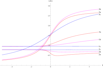
Figure 1: The curves (1a,b,c) and (2a,b,c) correspond to the gauge functions $\alpha(t,r)$ and $\beta(t,r)$ respectively. The curves (3a,b,c) depict the behavior of the gauge function $\tilde{\omega}(t,r)$ which has correct asymptotic limits $(0,\pi)$. The size parameter of Eguchi-Hanson instanton is set to be $a=1$. The subscripts (a,b,c) correspond to the fixed values of the space radius: $r=1,1.2,3$. The initial values for the gauge functions are taken to be close to the following asymptotic values $\alpha(t=-\infty)=\pi/4,~{}~{}\beta(t=-\infty)=\arccos(x^{1}/r),~{}~{}\tilde{\omega}(t=-\infty)=0$.

IV. Self-dual contortion

In generalized gravity models with contortion (torsion) the total Riemann-Cartan curvature can be decomposed into two parts in accordance with the split relationship (1) for the spin connection

$$R_{abcd}=\hat{R}_{abcd}+\tilde{R}_{abcd},$$

$$\hat{R}_{abcd}=\hat{D}_{\underline{b}}\varphi_{\underline{a}\underline{c}\underline{d}}+\varphi_{bc}^{~{}~{}\,\,e}\varphi_{aed}-(a\leftrightarrow b),$$

$$\tilde{R}_{abcd}=\hat{D}_{\underline{b}}K_{\underline{a}\underline{c}\underline{d}}+K_{bc}^{~{}~{}e}K_{aed}-(a\leftrightarrow b),$$ (73)

where, $\hat{R}_{abcd}$ is the Riemann curvature and $\hat{D}_{a}$ is a restricted covariant derivative containing only the Levi-Civita connection. The underlined indices stand for indices over which the covariantization is performed. Due to curvature decomposition (73) the classical vacuum can be defined by several ways. A simple definition of the vacuum in generalized Riemann-Cartan gravity includes two zero curvature conditions

$$\hat{R}_{abcd} = 0,$$

$$\tilde{R}_{abcd} = 0.$$ (74)

So that, in the space-time with a flat metric the tunneling is possible due to instanton configurations made of contortion. Non-trivial topological classes of contortion are provided by the same homotopy group $\pi_{3}(SO(1,3))$ as in Einstein gravity with vielbein. In this Section we consider possible configurations of self-dual contortion irrespectively on a concrete model of generalized Riemann-Cartan gravity. For simplicity, we suppose the vielbein to be flat, $e_{m}^{a}=\eta_{m}^{a}$. So that, $\gamma_{mcd}=K_{mcd}$ and the total Riemann-Cartan curvature $R_{abcd}$ coincides with the curvature $\tilde{R}_{abcd}$.

For the Riemann-Cartan curvature one can define two types of dual tensors using contraction of the antisymmetric tensor $\epsilon_{abcd}$ with either first or second index pair of $R_{mncd}$

$$R^{*}_{mnab} = \dfrac{1}{2}\epsilon_{abcd}R_{mncd},$$

$${}^{*}R_{mncd} = \dfrac{1}{2}\epsilon_{mnkl}R_{klcd}.$$ (75)

We define a self-dual Riemann-Cartan curvature as a tensor satisfying the double self-duality equations

$$R_{mncd} = R^{*}_{mncd},$$

$$R_{mncd} = {}^{*}R_{mncd}.$$ (76)

Using the ’t Hooft matrix $\eta^{i}_{cd}$ one can decompose any antisymmetric tensor $T_{ab}$ into self-dual and anti-self-dual parts

$$T_{ab}=\eta^{i}_{ab}S^{i}_{ab}+\bar{\eta}^{i}A^{i}_{ab}.$$ (77)

A self-dual Riemann-Cartan curvature can be written in the following form

$$R_{mncd}=\eta_{cd}^{i}R^{i}_{mn}.$$ (78)

The solution to the self-duality condition is provided by the self-dual spin connection with arbitrary functions $\gamma^{i}_{m}$

$$\gamma_{mcd}=\eta^{i}_{cd}\gamma^{i}_{m}.$$ (79)

In the case of Riemann geometry the self-duality condition implies the following expression for the Riemann curvature

$$R_{mncd} = \eta^{i}_{mn}\eta^{j}_{cd}P^{ij},$$

$$\eta_{mn}^{i} \equiv e^{a}_{m}e^{b}_{n}\eta^{i}_{ab},$$ (80)

where the tensor $P^{ij}$ must be symmetric due to the symmetry of the Riemann tensor under the replacement of first and second index pairs. The self-dual Riemann-Cartan curvature has the same form (80) with a non-symmetric tensor $P^{ij}$ in general. Let us construct some double self-dual contortion configurations using a proper ansatz.

I. We apply the ansatz

$$\gamma_{mcd}=\eta^{i}_{cd}\bar{\eta}^{i}_{mn}x^{n}f(\rho).$$ (81)

After substituting this ansatz into the Eqn. (80) one can find

$$\eta^{i}_{mn}P^{ij}=-2\bar{\eta}^{j}_{mn}(f+\rho^{2}f^{2})$$

$$+(\bar{\eta}^{j}_{mp}x_{n}-\bar{\eta}^{j}_{np}x_{m})x_{p}(\dfrac{f^{\prime}}{\rho}-2f^{2}).$$ (82)

Self-duality condition of the equation implies the constraint

$$\bar{\eta}^{k}_{mn}\eta^{i}_{mn}P^{ij}=0.$$ (83)

The last equation gives an ordinary differential equation

$$4f+\rho f^{\prime}+2\rho^{2}f^{2}=0$$ (84)

which has a solution

$$f(\rho)=-\dfrac{\lambda^{2}}{\rho^{2}(\rho^{2}+\lambda^{2})}.$$ (85)

This solution is analog to ’t Hooft-Polyakov one instanton solution in a singular gauge. Notice, that the tensor $P^{ij}$ is not symmetric

$$P^{ij}=-2\eta^{i}_{mn}\bar{\eta}^{j}_{mk}x^{n}x^{k}\dfrac{f}{\rho^{2}+\lambda^{2}},$$ (86)

so that the curvature $R_{mncd}$ represents essentially the Riemann-Cartan curvature. The contracted Riemann-Cartan curvatures are not vanished

$$R_{mncn}=\delta_{mc}P^{ii}+\eta^{k}_{mc}\epsilon^{kij}P^{ij},$$

$$R=4P^{ii}.$$ (87)

II. We choose the following ansatz

$$\gamma_{mcd}=\eta^{i}_{cd}\eta^{i}_{mn}x^{n}Q(\rho).$$ (88)

The solution to double self-duality equations for $R_{mncd}$ reads

$$Q=-\dfrac{1}{a^{2}+\rho^{2}}.$$ (89)

The curvature tensors have the following forms

$$R_{mncd}=\eta_{mn}^{i}\eta_{cd}^{i}\dfrac{2a^{2}}{(\rho^{2}+a^{2})^{2}},$$

$$R_{ab}=\delta_{ab}\dfrac{8a^{2}}{(\rho^{2}+a^{2})^{2}},$$

$$R=\dfrac{32a^{2}}{(\rho^{2}+a^{2})^{2}}.$$ (90)

The solution can be interpreted as a solution to the Riemann-Cartan analog of the Einstein equation with a non-constant cosmological term

$$R_{ab}=\Lambda(\rho)\delta_{ab}.$$ (91)

III. Let us construct a self-dual solution to self-duality condition for the conformal tensor $C_{mncd}$ (21) defined in terms of Riemann-Cartan curvature. We use the following ansatz

$$\gamma_{ncd}=\eta^{i}_{cd}\eta^{i}_{nk}x^{k}f(\rho)+\bar{\eta}^{i}_{cd}\bar{\eta}^{i}_{nk}x^{k}f(\rho).$$ (92)

Substituting the ansatz into the self-duality condition for the conformal tensor and requiring the condition of vanishing scalar Riemann-Cartan curvature $R=0$ one obtains a differential equation

$$R=-12(4f(\rho)+2\rho^{2}f^{2}(\rho)+\rho f^{\prime}(\rho))=0,$$ (93)

which has a solution

$$f(\rho)=-\dfrac{\lambda^{2}}{\rho^{2}(\rho^{2}+\lambda^{2})}.$$ (94)

This solution implies

$$C_{mncd}=0,$$

$$R=0,$$

$$R_{nd}=(\delta_{nd}\rho^{2}-4x_{n}x_{d})\dfrac{4\lambda^{2}}{\rho^{2}(\rho^{2}+\lambda^{2})^{2}}.$$ (95)

The solution is regular everywhere with a finite curvature invariant

$$R^{2}_{mncd}=\dfrac{1152\lambda^{4}}{(\rho^{2}+\lambda^{2})^{4}}.$$ (96)

The ansatz (92) contains two parts, each of them corresponds to self-dual contortion described by type II solution. So that the solution (94) can be interpreted as an analog to the instanton anti-instanton pair. Notice, that this solution is very similar to the conformally flat metric (23) considered in Section II. Notice, if we adopt the point of view that torsion is responsible for the microscopic structure of the space-time, and our Universe represents a classical macroscopic system, we can perform averaging procedure in the solutions (95) and (86) over all directions using the averaging prescription

$$<x_{n}x_{m}>=\dfrac{1}{4}\rho^{2}\delta_{nm}.$$ (97)

This implies vanishing of the Riemann-Cartan curvature. By this way the contortion may become unobservable at macroscopic level.

V. Discussion

We have shown explicitly that the Eguchi-Hanson instanton can provide tunneling between non-trivial topological vacuums represented by the vielbein in the case when the base space has topology of $RP^{3}$. Our main assumption is that the vielbein represents a more fundamental variable than the metric tensor. It might seem unexpected that the vacuum tunneling requires the space topology of $RP^{3}$, not $S^{3}$. An interesting discussion on which topology of the base space, $S^{3}$ or $RP^{3}$, should be accepted as a physical one, is presented in Ref. McInnes .

One should notice, that in our present Universe the vacuum tunneling is unlikely to be available since the Universe is not static and represents rather a macroscopic, noncoherent system in a quantum sense. However there is a possibility for experimental detecting the non-trivial vacuum structure. It is related to the presence of Adler-Bardeen-Jackiw (ABJ) axial anomaly, in a similar manner with quantum chromodynamics. A non-vanishing signature leads to the axial anomaly of the axial current for spin $\dfrac{1}{2}$ and spin $\dfrac{3}{2}$ particles. In the case of Eguchi-Hanson instanton the spin index $I_{1/2}$ of the Dirac operator is identically zero whereas the spin index $I_{3/2}$ is non-trivial. For the case of Fubini-Study instanton one has an axial ABJ anomaly fubini

$$\partial_{\mu}j^{5\mu}=\partial_{\mu}(\sqrt{g}e^{a\mu}\bar{\psi}\gamma_{a}\gamma_{5}\psi)=\dfrac{1}{4}RR^{*}.$$ (98)

Unfortunately in quantum gravity we don’t have an analogue of the pion decay coupling constant $f_{\pi}$ which could allow to measure the axial charge in gravity. As for the index $I_{3/2}$, there is a hope that spin 3/2 particles (like the $\Omega^{-}$ hyperon or the hypothetic particle gravitino) could open a way of direct detecting the non-trivial vacuum topology. Besides these pure thoughtful speculations one should notice that one has one indirect evidence why our space might have the topology of $RP^{3}$. This may come from the existence of the positive cosmological constant which provides the $RP^{3}$ topology of space-like hypersurfaces of the closed de Sitter universe.

The main assumption which we explore in our consideration of vacuum tunneling in Einstein gravity is that the vielbein represents a fundamental variable responsible for the quantum gravitational effects. If the Einstein gravity is an emergent phenomenon, i.e., it is an effective theory, then one should not quantize the vielbein which is a pure classic object by its geometric origin. Since a consistent quantum theory of gravity is unknown for the present moment, the question whether the vielbein or the torsion (or another object) is responsible for the quantum dynamics of gravity, remains open. One possible way to testify whether the vielbein can be more fundamental at quantum level than the metric is to perform experiment on detecting the gravitational analog of Aharonov-Bohm effect. We hope to study the theoretical framework for this in nearest future. Recently we have considered a gravity model with a topological phase where the vielbein does not play a role in quantum dynamics whereas the contortion (as a part of Lorentz connection) plays a fundamental role at quantum level pakijmp . In this connection our self-dual torsion configurations may have some physical applications.

Acknowledgements

One of authors (DGP) thanks Dr. Alex Nielsen for numerous useful discussions. The work is supported in part by Korean National Research Foundation (2008-314-C00069 and 2010-002-15640) and by the Brain Pool Program (032S-1-8) of KOSEF.

References

• (1) C. Rovelli, Quantum Gravity, Cambridge: Cambridge University Press, 2004.
• (2) L. Smolin, Three Roads to Quantum Gravity, New York: Basic Books, 2001.
• (3) H.W. Hamber, Quantum Gravitation. The Feynman Path Integral Approach, Springer-Verlag Berlin Heidelberg, 2009.
• (4) Y.M. Cho, Topology of Vacuum Space-Time, arXiv:hep-th/0703016.
• (5) S. Hawking, Euclidean Quantum Gravity, in Recent developments in gravitation, Procs. from CargΓ¨se, 1978. Eds. M. Levy and S. Deser. NATO Adv. Study Inst. Ser. Vol. B44 (1979) p.145.
• (6) G.W. Gibbons and S.W. Hawking, Phys. Lett. B78, 430 (1978).
• (7) F. Moraes, Phys. Lett. A214, 189 (1996).
• (8) M.O. Katanaev, Physics-Uspekhi 48(7) 675 (2005).
• (9) K. Kondo, in: Procs. 2nd Japan Natl. Congr. Applied Mechanics (Tokyo, 1952), Sci. Council of Japan, Tokyo (1953), pp.41-47.
• (10) R. Utiyama, Phys. Rev. 101, 1597 (1956).
• (11) T. W. B. Kibble, J. Math. Phys. 2, 212 (1961).
• (12) D. W. Sciama, Rev. Mod. Phys. 36, 463 (1964).
• (13) M. Carmelli, J. Math. Phys. 11, 2728 (1970).
• (14) R. Utiyama and T. Fukuyama, Prog. Theor. Phys. 45, 612 (1971).
• (15) Y. M. Cho, Phys. Rev. D14, 2521 (1976); see also 100 Years of Gravity and Accelerated Framesβ€”- The Deepest Insights of Einstein and Yang-Mills, edited by J. P. Hsu, World Scientific (Singapore) 2006.
• (16) Y. M. Cho, Phys. Rev. D14, 3335 (1976).
• (17) T. Eguchi and A. J. Hanson, Ann. Phys. 120, 82 (1979).
• (18) T. Eguchi and P.G.O. Freund, Phys. Rev. Lett. 37, 1251 (1976).
• (19) S.W. Hawking, Phys. Lett. B195, 337 (1987).
• (20) H. Culetu, Gen. Relat. Grav. 26, 282 (1994),
• (21) Y. Agaoka, Procs. Amer. Math. Soc. 123, 3519 (1995).
• (22) P. van Baal and A. Wipf, Phys. Lett. B515, 181 (2001).
• (23) Y. M. Cho, Phys. Lett. B644, 208 (2007).
• (24) G. ’t Hooft, Phys. Rev. Lett. 37, 8 (1976).
• (25) R. Jackiw and C. Rebbi, Phys. Rev. Lett. 37, 172 (1976).
• (26) C. Callan, R. Dashen, and D. G. Gross, Phys. Lett. B63, 334 (1976).
• (27) Y. M. Cho, Phys. Lett. B81, 25 (1979).
• (28) B. McInnes, JHEP 0309:009 (2003).
• (29) Y.M. Cho, D.G. Pak and B.S. Park, Int. J. Mod. Phys. A25, 2867 (2010).