Studies on X-ray Thomson Scattering from Antiferroquadrupolar Order in TmTe

Abstract

We study Thomson scattering from the antiferroquadrupole ordering phase in TmTe. On the basis of the group theoretical treatment, we classify the selection rules of the scattering intensity governed by the orientation of the scattering vector G. Then, numerical verification is performed by invoking the ground states which are deduced from a $J=\frac{7}{2}$ multiplet model. The obtained intensity varies drastically depending on the magnitude and direction of G. We also calculate the scattering intensities under the applied field for $\textbf{H}\parallel(001)$ and $(110)$. Their results behave differently when the orientation of G is changed, which is ascribed to the difference of their primary order parameters; $O_{2}^{0}$ and $O_{2}^{2}$ for $\textbf{H}\parallel(001)$ and $(110)$, respectively. We make critical comparisons between our results for TmTe and the experimental ones for CeB₆. First, we assert that the intensities expected from TmTe at several forbidden Bragg spots are sufficient enough to be experimentally detected. Second, their intensities at $\left(\frac{7}{2}\frac{1}{2}\frac{1}{2}\right)$ differ significantly and may be attributed to the difference of the order parameters between the $\Gamma_{3}$-type ($O_{2}^{2}$ and $O_{2}^{0}$) and $\Gamma_{5}$-type ($O_{yz},O_{zx}$, and $O_{xy}$) components, respectively.

1 Introduction

The interplay of orbital and spin degrees of freedom in localized magnetic materials brings about a wide variety of interesting phenomena. In many $f$-electron systems, due to the strong coupling between the spin and orbital angular momenta, the states are described by the multiplets of the total angular momentum $J$. When the symmetry exhibited by the system is sufficiently high, the multiplet enables the higher rank multipoles as well as the dipole (rank one) be active. In fact, various experimental and theoretical studies have been devoted to clarify the nature of the ordered phase of multipole order parameters with rank higher than one.[1, 2] Among the most investigated systems, the materialization of the antiferroquadrupole (AFQ) ordering phase has been established in the materials such as CeB₆ and DyB₂C₂.

Among many experimental probes, scattering experiments such as resonant X-ray scattering (RXS) and (non-resonant X-ray) Thomson scattering provide very powerful tools to reveal the natures of the higher rank multipolar ordering phase. For example, the AFQ ordering phases in CeB₆ and DyB₂C₂ are investigated in detail by means of RXS[3, 4, 5, 6, 7] and Thomson scattering.[4, 10, 8, 9]

On the other hand, the situation of TmTe may still be rudimentary. This material is believed to show the AFQ order below $T_{\textrm{Q}}=1.8$ K.[11] Although many evidences for the AFQ order were gathered in terms of various experimental probes,[12, 13, 14] there remain some important issues unsettled yet. For instance, the crystal electric field (CEF) level scheme, the component of the primary order parameter, the nature of the multipolar interaction, and so on. In order to address such issues, the approaches in terms of the scattering experiments may be helpful. In our previous work, we have determined the CEF level scheme as $\Gamma_{8}-\Gamma_{6}-\Gamma_{7}$ and analyzed some properties expected from the azimuthal angle dependence of the RXS intensity, which are useful to distinguish the type of the order parameter.[15]

In this paper, we carry out some investigations on Thomson scattering expected from the AFQ phase in TmTe. After introducing the theoretical framework to calculate the scattering intensity, we first proceed to classify the selection rules of intensity governed by the direction of the scattering vector. In the absence of the applied field, such selection rules as well as the domain consideration determine the whole intensity. The intensity exhibits the strong dependence on the magnitude and orientation of the scattering vector. We verify the qualitative results with the numerical calculation performed on the theoretical model developed in our previous paper.[15] We also investigate how the application of the external field alters the scattering intensity. When the field is applied along $(001)$ and $(110)$, the primary order parameters derived from the model are $O_{2}^{0}=1/2(2J_{z}^{2}-J_{x}^{2}-J_{y}^{2})$ and $O_{2}^{2}=\sqrt{3}/2(J_{x}^{2}-J_{y}^{2})$, respectively. We find their intensities show different behaviors as a function of the orientation of the scattering vector, reflecting the difference of their primary order parameters.

We also try to compare the present results with those obtained for CeB₆.[4, 16] Although both TmTe and CeB₆ exhibit the AFQ ordering phases, it is said the components of the order parameters are different from each other; the $\Gamma_{3}$-type ($O_{2}^{2}$ and $O_{2}^{0}$) in the former and the $\Gamma_{5}$-type ($O_{yz},O_{zx}$, and $O_{xy}$) in the latter. Here, $O_{yz}=\sqrt{3}/{2}(J_{y}J_{z}+J_{z}J_{y}),O_{zx}=\sqrt{3}/2(J_{z}J_{x}+J_{x}J_{z})$, and $O_{xy}=\sqrt{3}/2(J_{x}J_{y}+J_{y}J_{x})$. Our investigation tells that: First, there is a realistic chance to experimentally detect the Thomson scattering signals in TmTe. Second, the intensities show different tendency in both materials at several forbidden Bragg spots, which may be attributed to difference of the component of the order parameters.

This paper is organized as follows. Section 2 is spent to introduce a theoretical framework in order to calculate the Thomson scattering intensity. In §3, we briefly summarize the CEF scheme concluded from our previous paper and explain the ground state both in the absence and presence of the applied magnetic field. In §4, we derive some properties of the Thomson scattering intensities from the AFQ phase in TmTe, for instance, its dependence on the direction of the scattering vector and applied magnetic field. A comparison of the present results and those obtained for CeB₆ is also found. Finally, §5 is devoted to concluding remarks. Note that a very early stage of the present work is published elsewhere.[17]

2 Scattering Amplitude of Thomson Scattering

The cross section of Thomson scattering is defined as

$$\left(\frac{d\sigma}{d\Omega}\right)=\left|r_{0}(\mbox{\boldmath{$\epsilon$}}\cdot\mbox{\boldmath{$\epsilon$}}^{\prime})f(\textbf{G})\right|^{2},$$ (1)

where $r_{0}$ is the classical electron radius. The directions of polarization for the incident and scattered photons are denoted by $\epsilon$ and $\mbox{\boldmath{$\epsilon$}}^{\prime}$, respectively. The inner product $\mbox{\boldmath{$\epsilon$}}\cdot\mbox{\boldmath{$\epsilon$}}^{\prime}$ gives non-zero value only when the photon polarization is unrotated; being unity in the $\sigma-\sigma^{\prime}$ channel while $\cos(2\theta_{\textrm{B}})$ in the $\pi-\pi^{\prime}$ channel where $\theta_{\textrm{B}}$ is the Bragg angle. The scattering amplitude is described as $f(\textbf{G})$ where the scattering vector is defined as $\textbf{G}=\textbf{k}^{\prime}-\textbf{k}$ with k and $\textbf{k}^{\prime}$ being the wave vectors of the incident and scattered photons, respectively.

We consider the localized electron system with the $(4f)^{N}$ configuration. The scattering amplitude may be given by a sum of the contributions from the localized $4f$ electrons:

$$f(\textbf{G}) = \frac{1}{\sqrt{N_{0}}}\sum_{j}\sum_{n=1}^{N}\sum_{\mu}p_{\mu}(j)\textrm{e}^{-i\textbf{G}\cdot\textbf{R}_{j}}$$ (2)

$$\times \langle 0_{\mu}(j)|\textrm{e}^{-i\textbf{G}\cdot\textbf{r}_{n}}|0_{\mu}(j)\rangle,$$

where $N_{0}$ is the number of Tm ion sites. Electron position $\textbf{r}_{n}$ is measured in the coordinate system centered at each Tm site $j$. The $|0_{\mu}(j)\rangle$ refers to the ground state of the $N$ electrons with probability $p_{\mu}(j)$ where $\mu$ distinguishes possible degeneracies. We proceed to rewrite the expectation value part in eq. (2), hence we omit the labels $j$ and $\mu$ in the following.

The numerical evaluation of the amplitude can be easily performed by utilizing the so-called Rayleigh expansion of the exponential[18]

$$\textrm{e}^{-i\textbf{G}\cdot\textbf{r}}=4\pi\sum_{k=0}^{\infty}(-i)^{k}j_{k}(Gr)\sum_{k_{z}=-k}^{k}Y_{k,k_{z}}(\Omega)Y_{k,k_{z}}^{\star}(\Omega_{G}),$$ (3)

where $j_{k}$ means the $k$-th order spherical Bessel function and $Gr=|\textbf{G}||\textbf{r}|$. The solid angles of r and G are represented as $\Omega$ and $\Omega_{G}$, respectively. Note that the similar treatments are found in the literatures analyzing Thomson scattering of X-rays from the ordering phase in CeB₆ for $f^{1}$-configuration.[20, 16, 19]

In expanding the ground state, we employ the total angular momentum basis involving the radial part, $|J,J_{z}\rangle$, as follows:

$$|0\rangle=\sum_{J_{z}=-J}^{J}a(J_{z})|J_{z}\rangle.$$ (4)

where we denote $\left|J,J_{z}\right\rangle$ as $|J_{z}\rangle$. The state $|J_{z}\rangle$ can be expanded by means of the Slater determinant constructed by the one-electron spin orbitals for $N$ electrons. Generally, the evaluation of eq. (2) from the $N$-electron Slater determinant is tedious,[21] and one can employ the formalism on the basis of the Stevens operator equivalence method.[22] When $N=1$ and $13$, however, the situations are quite simple and we can carry out the evaluation easily. Reflecting the fact that Tm²⁺ ion is in the $f^{13}$-configuration, we restrict $N=13$ in the following.

Then, the Slater determinant for thirteen electrons is specified by the quantum numbers, orbital ($\ell_{z}$) and spin ($s_{z}$) angular momenta, for a single hole which is the lone unoccupied one-electron spin orbital in each determinant. Hence the state $|J_{z}\rangle$ is written in the form of

$$|J_{z}\rangle=\sum_{\ell_{z}=-\ell}^{\ell}\sum_{s_{z}=-s}^{s}C(J,J_{z}:\ell,-\ell_{z};s,-s_{z})|\ell\ell_{z},ss_{z}\rangle,$$ (5)

where $C(JJ_{z}:\ell\ell_{z},ss_{z})$ is the Clebsch-Gordan (CG) coefficient with $\ell=3$ and $s=\frac{1}{2}$ for an $f$ electron. The ket $|\ell\ell_{z},ss_{z}\rangle$ stands for the Slater determinant for thirteen electrons labeled by the hole quantum numbers $\ell_{z}$ and $s_{z}$. Note that when the ket means one-electron spin orbital, the minus signs in the CG coefficient of eq. (5) disappear. The one-electron spin orbital is described by the product of radial part $R_{4f}(r)$, angular part $Y_{\ell,\ell_{z}}$, and spin part $\chi_{s,s_{z}}$. By combining this and eq. (4) with eq. (5), we can continue the evaluation of the expectation value of eq. (3), the detail of which is relegated to Appendix. The result is summarized as

$$\sum_{n=1}^{13}\langle 0|\textrm{e}^{-i\textbf{G}\cdot\textbf{r}_{n}}|0\rangle=14\langle j_{0}(G)\rangle-\sum_{J_{z},J_{z}^{\prime}}a^{\star}(J_{z})a(J_{z}^{\prime})f_{J_{z},J_{z}^{\prime}}.$$ (6)

Here, we have introduced the amplitude matrix as

$$f_{J_{z},J_{z}^{\prime}} \equiv \sum_{\ell_{z},\ell_{z}^{\prime},s_{z}}C(JJ_{z}:\ell\ell_{z},ss_{z})C(JJ_{z}^{\prime}:\ell\ell_{z}^{\prime},ss_{z})$$ (7)

$$\times \sqrt{4\pi}\sum_{k=0}^{\infty}(-i)^{k}\sqrt{2k+1}\langle j_{k}(G)\rangle Y_{k,\ell_{z}-\ell_{z}^{\prime}}(\Omega_{G})$$

$$\times c^{k}(\ell\ell_{z},\ell\ell_{z}^{\prime}),$$

where the Gaunt coefficient is defined by

$$c^{k}(\ell\ell_{z},\ell\ell_{z}^{\prime})=\sqrt{\frac{4\pi}{2k+1}}\int Y_{\ell,\ell_{z}}^{\star}(\Omega)Y_{k,\ell_{z}-\ell_{z}^{\prime}}(\Omega)Y_{\ell,\ell_{z}^{\prime}}d\Omega,$$ (8)

and

$$\langle j_{k}(G)\rangle=\int_{0}^{\infty}r^{2}j_{k}(Gr)R_{4f}^{2}(r)dr.$$ (9)

Since the first term in eq. (6) is independent of the ground state, it has no contribution to the scattering intensity as far as G is chosen as antiferro-type spot.

The Gaunt coefficients are evaluated by means of the Wigner $3j$ symbols. In the present case of $f$ electron system with $\ell$ being fixed to three, only the terms for $k=0,2,4$, and $6$ are relevant. As a consequence, $f_{J_{z},J_{z}^{\prime}}$ and eventually the scattering amplitude itself are invariant under the transformation $\textbf{G}\leftrightarrow-\textbf{G}$. In this context, we do not discriminate between G and $-\textbf{G}$ in the present work, in particular, when we perform numerical evaluation of the scattering intensities. Notice that we can verify the symmetry relations exhibited by the amplitude matrix elements as follows

$$f_{J_{z},J_{z}^{\prime}}=f_{J_{z}^{\prime},J_{z}}^{\star}=(-)^{J_{z}-J_{z}^{\prime}}f_{-J_{z},-J_{z}^{\prime}}^{\star}=(-)^{J_{z}-J_{z}^{\prime}}f_{-J_{z}^{\prime},-J_{z}}.$$ (10)

A remaining task is to calculate the coefficient $a(J_{z})$’s. We briefly summarize the methods and results in the next section.

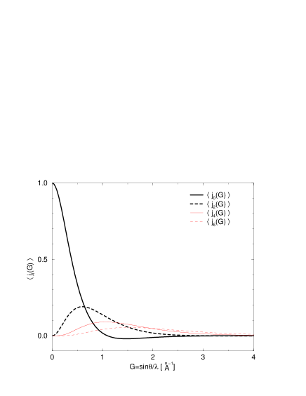
Figure 1: (Color online) Radial integrations of spherical Bessel function $\langle j_{k}(G)\rangle$ for divalent Tm ion as a function of $G=|\textbf{G}|$. The bold solid (black), bold dotted (black), thin solid (red), and thin dotted (red) lines for $k=0,2,4$, and $6$, respectively.

3 Ground State

Thulium telluride (TmTe) is a magnetic semiconductor crystallized in a cubic, NaCl structure with a lattice constant of $a=6.35\textrm{\AA}$. The Tm ion is in a divalent state with one $4f$ hole [$(4f)^{13}$] configuration (${}^{2}F_{\frac{7}{2}}$). The radial part of the wave function $R_{4f}(r)$ we use is calculated within the Hartree-Fock approximation for Tm²⁺.[23] The $\langle j_{k}(G)\rangle$’s are evaluated by means of $R_{4f}(r)$ as shown in Fig. 1. Then, the angular part of the wave functions are prepared as follows.

Under the cubic CEF potential, the ground multiplet spanned by $J=\frac{7}{2}$ subspace is split into two doublets $\Gamma_{6}$ and $\Gamma_{7}$ and a quartet $\Gamma_{8}$. Since their total separation is believed to be around 15 K,[12] we should retain all the bases. In the previous paper, we have introduced a model Hamiltonian on the $J=7/2$ multiplet basis to describe the phase diagram for TmTe.[15] Analyzing carefully an interplay among the CEF potential, the Zeeman energy, and multipolar interactions, we have concluded that the $\Gamma_{3}$ AFQ order parameter and a CEF level structure $\Gamma_{8}$-$\Gamma_{6}$-$\Gamma_{7}$ naturally explain the observed field dependence and anisotropy of the phase diagram. In the present analysis, the intensity of X-ray scattering is calculated by using the mean-field ground state derived from the same Hamiltonian. Here, let us summarize the Hamiltonian and its mean-field results briefly.

The basic assumption in the model is that the original fcc lattice of Tm ions can be decoupled to four distinct sc sublattices.[24] Then, the model on the sc lattice is defined by a sum of three parts, $H=H_{\rm C}+H_{\rm Z}+H_{\rm Q}$, where

$$H_{\rm C} =W\sum_{i}\left[x\frac{O_{4}(i)}{F_{4}}+(1-|x|)\frac{O_{6}(i)}{F_{6}}\right],$$ (11a)

$$H_{\rm Z} =-g\mu_{B}\sum_{i}\mbox{\boldmath{$J$} }(i)\cdot\mbox{\boldmath{$H$} },$$ (11b)

$$H_{\rm Q} =D_{\rm Q}\sum_{\langle ij\rangle}\left[O_{2}^{0}(i)O_{2}^{0}(j)+O_{2}^{2}(i)O_{2}^{2}(j)\right].$$ (11c)

$H_{\rm C}$ is the CEF Hamiltonian defined in ref. Lea1962, and $H_{\rm Z}$ is the Zeeman energy in the magnetic field $H$ with $g=8/7$ being the Landé $g$ factor for $J=7/2$. The $\Gamma_{3}$ AFQ interaction relevant for TmTe is given by $H_{\rm Q}$, where the summation over $\langle ij\rangle$ is restricted to the nearest-neighbor sites in the sc lattice. For simplicity we do not consider influences of field-induced multipoles in this model Hamiltonian.

Concerning the parameters in the CEF Hamiltonian $H_{\rm C}$, we assume $W=-0.417$K and $x=0.5$ which lead to a level scheme $\Gamma_{8}$(0K)-$\Gamma_{6}$(5K)-$\Gamma_{7}$(10K). This is nothing but scheme (b) in ref.Shiina2008, namely the most promising CEF level scheme for TmTe. The quadrupole coupling constant is determined so as to give the transition temperature $T_{\rm Q}=4$K at zero field, for the fixed CEF level scheme. We expect that the transition temperature must be suppressed and becomes closer to the real value $T_{\rm Q}=1.8$K when the strong fluctuation is taken into account.

Applying the mean field approximation for the AFQ interaction, one can determine the stable order parameters depending on the direction of the magnetic fields.[15] It is shown that the $O_{2}^{0}$ order appears in $\mbox{\boldmath{$H$} }||(001)$ whereas the $O_{2}^{2}$ order is stabilized in $\mbox{\boldmath{$H$} }||(110)$. On the other hand, $O_{2}^{0}$ and $O_{2}^{2}$ are almost degenerate at zero field and in $\mbox{\boldmath{$H$} }||(111)$ due to high symmetry. Thereby, we assume the $O_{2}^{2}$ order at zero field in this study, because the observed field-induced antiferromagnetic structure in $\mbox{\boldmath{$H$} }||(110)$ indicating $O_{2}^{2}$ are continuously connected to the zero field.[13] These mean field analyses obviously provide the ground state wave function at each sublattice site, which can be used to calculate the X-ray scattering intensity at zero temperature.

Finally, we shall briefly comment on the properties of the AFQ domains within the model described by eqs. (11a) $\sim$ (11c). As discussed above, the model leads to a simple antiferro-type structure characterized by a wave vector $\textbf{K}_{1}=(111)$ in units of $\pi/a$. Although this wave vector is unique on the $sc$ lattice, it allows degeneracy on the $fcc$ lattice, with $\textbf{K}_{2}=(\overline{1}11)$, $\textbf{K}_{3}=(1\overline{1}1)$, and $\textbf{K}_{4}=(\overline{11}1)$. This degeneracy is equivalent to the degeneracy when combining four decoupled $sc$ sublattices to a single $fcc$ lattice. Therefore, the four $K$ domains remain to be unchanged in the present model even when the magnetic field is applied. The stability of the $K$ domains is determined exclusively by a subtle inter-sublattice interaction.[26] In the present paper, we will present the results of each $K$ domain and will not discuss details on the stability problems.

4 Thomson Scattering Intensities

4.1 Remarks on scattering from K domain

The scattering vector in Thomson scattering to detect the antiferro-type ordering pattern in TmTe is simply described as $\textbf{G}=(2h+1,2k+1,2\ell+1)$ with $h,k$, and $\ell$ being integers, in units of $\pi/a$. In this case, the phase factor appeared in eq. (2) becomes $\textrm{e}^{-i\textbf{G}\cdot\textbf{R}_{j}}=+1$ or $-1$ depending on which sublattice $\textbf{R}_{j}$ belongs to. We can verify that for any antiferro-type G, there exists only one $m$ among $1\sim 4$ which satisfies $\textrm{e}^{-i\textbf{G}\cdot\textbf{R}_{j}}=\textrm{e}^{-i\textbf{K}_{m}\cdot\textbf{R}_{j}}$ at every $\textbf{R}_{j}$. Thus, the scattering amplitude remains finite only from the $K$-domain which satisfies this relation. In this sense, the scatterings from distinct $K$-domains should be identified by the corresponding scattering vectors.

Here, we calculate the intensity for the perfect single $K$-domain, which is picked up by the scattering vector. This should be kept in mind when we compare the calculated results with the experimental ones. If each $K$-domain would have nearly the same population, our results overestimate factor four.

4.2 Dependence on the direction of scattering vector

We exploit a group theoretical analysis on the scattering amplitude $f(\textbf{G})$ [eq. (2)]. The amplitude is invariant under the symmetry operations keeping both crystal and G unchanged. Under cubic symmetry ($O_{h}$), $f(\textbf{G})$ is constructed by the quantities belonging to the identical ($\Gamma_{1}$) representation in a point group $O_{h}\times\textbf{G}$. Here, some symmetry operations in $O_{h}$ are forbidden by assuming an artificial strain along G in $O_{h}\times\textbf{G}$. Since $f(\textbf{G})$ is expanded by a linear combination of the terms with even rank, only the even rank multipole operators belonging to the $\Gamma_{1}$ representation in $O_{h}\times\textbf{G}$ contribute to the scattering intensity. This is a striking difference compared with a starting point of the similar analysis for the magnetic neutron scattering form factor where the unprojected scattering operator behaves as the odd rank multipole operators.[27] In the present case of the antiferro-type ordering phase, it corresponds to detect the $\Gamma_{1}$ representation from rank two operator. This is easily confirmed by re-expressing eq. (6) as

$$\sum_{n=1}^{13}\langle 0|\textrm{e}^{-i\textbf{G}\cdot\textbf{r}_{n}}|0\rangle=13\langle j_{0}(G)\rangle$$ (12)

$$- \sum_{k=2,4,6}\sum_{J_{z},J_{z}^{\prime}}a^{\star}(J_{z})a(J_{z}^{\prime})B^{k}(J_{z},J_{z}^{\prime})\langle j_{k}(G)\rangle,$$

where coefficient $B^{k}(J_{z},J_{z}^{\prime})$ is obtained by eliminating expression $\sum_{k=0}^{\infty}\langle j_{k}(G)\rangle$ from the right hand side of eq. (7). The first term is canceled by the contributions from two sublattices, which leaves the expansion starting with the term $k=2$.

Equation (12) indicates the presence of the contributions from the terms of rank four and six. However, qualitative behavior of the whole intensity is well understood by that from the leading term proportional to $\langle j_{2}(G)\rangle$. The reasons are two fold. First, because the symmetry properties of the coefficients $B^{2}(J_{z},J_{z}^{\prime}),B^{4}(J_{z},J_{z}^{\prime})$, and $B^{6}(J_{z},J_{z}^{\prime})$ deduced from relation similar to eq. (10) are the same one another, the latter two terms do not give rise to qualitatively new properties which are absent for $B^{2}(J_{z},J_{z}^{\prime})$ term alone. It means their influence on the total intensity is quantitative, not qualitative. Second, it turns out from the numerical calculations in the following subsections that the contribution from the term proportional to $\langle j_{2}(G)\rangle$ dominates the intensity. Therefore, though our numerical calculation shall include the contributions from the terms with rank four and six, we proceed to make a group theoretical consideration deduced only from the rank two term and derive some selection rules which qualitatively explain the behavior of the whole intensity.

In a point group $O_{h}$, rank two quadrupole operators are $\Gamma_{3}$-type $(O_{2}^{0},O_{2}^{2})$ and $\Gamma_{5}$-type $(O_{yz},O_{zx},O_{xy})$. For $\textbf{G}\parallel(001),(111)$, and $(110)$, the components to be invariant under $O_{h}\times\textbf{G}$ are $O_{2}^{0}$, $(O_{yz}+O_{zx}+O_{xy})/\sqrt{3}$, and $O_{2}^{0}$ and $O_{xy}$, respectively. Note that this is the same as symmetry lowering of quadrupoles by the magnetic field, as discussed in ref. Shiina1997. Although antiferro-type G spot does not exist in the $(001)$ nor $(110)$ directions, they are interpreted as the limiting cases of the spots, for example, at $\textbf{G}=(1,1,2h+1)$ and $(2h+1,2h+1,1)$, respectively.

In the absence of the applied field, the order parameter is $O_{2}^{2}$ as explained in the previous section. In the cubic symmetry, two more independent primary order parameters are obtained by rotating $O_{2}^{2}$ by an angle $\pm 2\pi/3$ about the wave vector specifying the $K$-domain. The domains specified by these primary order parameters are called as $S$-domains. In the $K_{1}$-domain, for instance, the primary order parameters of three $S$-domains become $O_{2}^{2}$, $(\sqrt{3}O_{2}^{2}-O_{2}^{0})/2$, and $-(\sqrt{3}O_{2}^{2}-O_{2}^{0})/2$. Then, for a given G, if the $\Gamma_{1}$ representation contains $O_{2}^{0}$ and/or $O_{2}^{2}$, we can expect the Thomson scattering intensity remains finite. We proceed to our investigation assuming that three $S$-domains have the equal population in each $K$-domain. In the following, the numerical results are presented for the $\sigma-\sigma^{\prime}$ channel when unspecified.

Let us consider $\textbf{G}||(111)$ at first. It is clear that the $\Gamma_{1}$ representation $(O_{yz}+O_{zx}+O_{xy})/\sqrt{3}$ in $O_{h}\times\textbf{G}$ is not involved in the order parameter. Therefore, the scattering is forbidden in this case. Then, we examine the intensity at $\textbf{G}=(2h+3,2h+1,2h+1)$, which approaches to $\textbf{G}\parallel(111)$ in the limit of $h\rightarrow\infty$. As shown in Fig. 2, the intensity obtained at $(2h+3,2h+1,2h+1)$ is very tiny as expected.

Second, we consider $\textbf{G}=(001)$. Two of the three $S$-domains whose order parameters include $O_{2}^{0}$ can give finite intensities in this case. Obviously, the same result is expected for $\textbf{G}=(100)$ and (010). In Fig. 2, we plot the calculated intensity at $(2h+1,1,1)$, together with the result for continuous $\textbf{G}\parallel(100)$. The latter is evaluated by assuming $\textrm{e}^{-i\textbf{G}\cdot\textbf{R}_{j}}$ in eq. (2) being $+1$ or $-1$ corresponding to $\textbf{R}_{j}$’s sublattice. As seen from Fig. 2, the limiting curve is in good accordance with the intensities obtained at the real antiferro-type spots $\textbf{G}=(2h+1,1,1)$ even when $h$ is small.

Then, for another limiting case, $\textbf{G}\parallel(110)$, the discussion similar to that for $(100)$ is easily confirmed. That is, the direction $(110)$ is considered as the limiting direction of an antiferro-type spot $\textbf{G}=(2h+1,2h+1,1)$. The scattering intensity at $(2h+1,2h+1,1)$ is equal to those at the corresponding spots at $(1,2h+1,2h+1)$ and $(2h+1,1,2h+1)$. We verify these results and display the curve together with that for $\textbf{G}\parallel(110)$ also in Fig. 2.

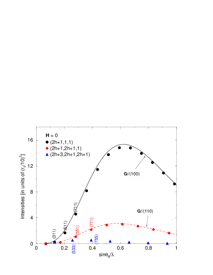
Figure 2: (Color online) The Thomson scattering intensities per Tm ion under no applied field in the $\sigma-\sigma^{\prime}$ channel. The (black) circles, (red) diamonds, and (blue) triangles are the intensities for $\textbf{G}=(2h+1,1,1),(2h+1,2h+1,1)$, and $(2h+3,2h+1,2h+1)$, respectively, with $h=0,1,2,\cdots$. The (black) solid and (red) dotted lines show the limiting curve for $\textbf{G}\parallel(100)$ and $(110)$, respectively.

4.3 Dependence on the direction of applied field

When external field is applied to the system, usually, degeneracies associated with the $S$-domains are lifted depending on the direction of the field, which also removes the equivalence of the intensities under no external field for several high-symmetry G directions. For instance, for $\textbf{H}\parallel(001)$, the primary order parameter of the ground state becomes $O_{2}^{0}$. The identity representation in $O_{h}\times\textbf{G}$ is $O_{2}^{0},(\sqrt{3}O_{2}^{2}-O_{2}^{0})/2$, and $(-\sqrt{3}O_{2}^{2}-O_{2}^{0})/2$ for $\textbf{G}\parallel(001),(100)$, and $(010)$, respectively. Then, we expect the intensities for $\textbf{G}\parallel(100)$ and $(010)$ are equivalent and weaker than that for $\textbf{G}\parallel(001)$. For corresponding antiferro-type $\textbf{G}=(1,1,2h+1),(2h+1,1,1)$, and $(1,2h+1,1)$, the intensities for the latter two are the same, which are weaker than that for the former one as displayed in Fig. 3 (a). Next, we consider the limiting directions $\textbf{G}\parallel(110),(011)$, and $(101)$. Since the identity representations belonging to the $\Gamma_{3}$ block for them are equivalent to those for $\textbf{G}\parallel(001),(100)$, and $(010)$, respectively, the same relations hold. That is, the intensities for $\textbf{G}\parallel(011)$ and $(101)$ are the same, which are weaker than that for $\textbf{G}\parallel(110)$. Similarly, the intensities at $\textbf{G}=(1,2h+1,2h+1)$ and $(2h+1,1,2h+1)$ spots are the same, which are weaker than the one at $(2h+1,2h+1,1)$ spot. The intensities at $\textbf{G}=(2h+3,2h+1,2h+1)$ are negligible and we omit them from Fig. 3 (a).

For $\textbf{H}\parallel(110)$, the primary order parameter of the ground state is $O_{2}^{2}$. From the analysis for the limiting cases, the series $\textbf{G}\parallel(100)$ and $(010)$ include $O_{2}^{2}$ as the $\Gamma_{1}$ representation while $\textbf{G}\parallel(001)$ does not. Then, the intensities at $\textbf{G}=(2h+1,1,1)$ and $(1,2h+1,1)$ are expected to be the same while tiny intensity, if any, is brought about at $\textbf{G}=(1,1,2h+1)$. These tendencies are confirmed numerically as shown in Fig. 3 (b). Similarly, the intensities at $\textbf{G}=(1,2h+1,2h+1)$ and $(2h+1,1,2h+1)$ give the same values while that at $\textbf{G}=(2h+1,2h+1,1)$ is essentially zero.

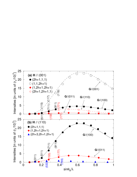
Figure 3: (Color online) The Thomson scattering intensities per Tm ion under the applied field along (a) $(001)$ and (b) $(110)$ directions in the $\sigma-\sigma^{\prime}$ channel. The (black) filled and open circles are the intensities for $\textbf{G}=(2h+1,1,1)$ and $(1,1,2h+1)$, respectively, with $h=0,1,2,\cdots$. While the (red) filled and open diamonds, and (blue) filled triangles are those for $\textbf{G}=(1,2h+1,2h+1),(2h+1,2h+1,1)$, and $(2h+3,2h+1,2h+1)$, respectively. The (black) solid and dotted lines show the limiting curves for $\textbf{G}\parallel(100)$ and $(001)$, respectively. The (red) solid and dotted lines show the limiting curves for $\textbf{G}\parallel(011)$ and $(110)$, respectively.

4.4 Comparison with the CeB₆’s results

Two $f$ electron systems CeB₆ and TmTe share some apparent similarities. First, both materials are cubic systems. Second, they are considered as the one $f$-particle systems: In CeB₆, Ce³⁺ ion is in the $f^{1}$ configuration in the electron picture, while in TmTe, Tm²⁺ ion is in the $\underline{f}^{1}$ configuration in the hole picture. Third, they both exhibit AFQ ordering phases below the critical temperature. On the basis of these nominal resemblances, our main focus is to find the differences they may show. One obvious difference is the $J$ value. Owing to the Hund’s rule, $J=\frac{5}{2}$ and $\frac{7}{2}$ in CeB₆ and TmTe, respectively. Under the cubic circumstances and inferred from the CEF splitting, their ground states are spanned by one $\Gamma_{8}$ quartet in the former, and two doublets ($\Gamma_{6}$ and $\Gamma_{7}$) and one $\Gamma_{8}$ quartet in the latter. Those differences may reflect on the differences of the Thomson scattering amplitude between TmTe and CeB₆. Due to the difference of the value of $J$ and corresponding difference of the bases used, CeB₆ does not include the term proportional to $\langle j_{6}(G)\rangle$ while TmTe does.

Other than this difference, their differences tend to be quantitative ones. Among them, we examine the experimental results presented by Yakhou et al. They reported the ratios of the Thomson scattering intensities at $\textbf{G}=(511)$ and $(711)$ to that at $\textbf{G}=(533)$ from the AFQ phase in CeB₆ under no applied field.[4] The results are $I_{\pi-\pi^{\prime}}^{\textrm{exp.}}(511)/I_{\pi-\pi^{\prime}}^{\textrm{exp.}}(533)\simeq I_{\pi-\pi^{\prime}}^{\textrm{exp.}}(711)/I_{\pi-\pi^{\prime}}^{\textrm{exp.}}(533)\simeq 0.02$ in the $\pi-\pi^{\prime}$ channel. Here, the scattering intensity in the $\mu-\mu^{\prime}$ channel at scattering vector $\textbf{G}=(2h+1,2k+1,2\ell+1)$ is denoted as $I_{\mu-\mu^{\prime}}(2h+1,2k+1,2\ell+1)$. With and without the superscript ’exp.’ distinguish between the experimental data and the theoretical ones, respectively. The intensities measured in the $\pi-\pi^{\prime}$ channel involve the factor $\cos^{2}(2\theta_{\textrm{B}})$, which depends on the photon energy. When we compare the experimental data for CeB₆ with those obtained from TmTe, it is convenient to eliminate this factor, which leads to the ratios expected from the measurement in the $\sigma-\sigma^{\prime}$ channel. Then, the experimental data are interpreted as $I_{\sigma-\sigma^{\prime}}^{\textrm{exp.}}(511)/I_{\sigma-\sigma^{\prime}}^{\textrm{exp.}}(533)\simeq 1.22$ and $I_{\sigma-\sigma^{\prime}}^{\textrm{exp.}}(711)/I_{\sigma-\sigma^{\prime}}^{\textrm{exp.}}(533)\simeq 0.01$ in the $\sigma-\sigma^{\prime}$ channel.

To begin with, we comment on a possibility of the experimental detection of the Thomson scattering signals from TmTe. The strongest signal in Yakhou et al.’s data for CeB₆ is obtained at $(533)$.[4] Since they did not present the absolute value of $I_{\pi-\pi^{\prime}}^{\textrm{exp.}}(533)$, we interpret the theoretical intensity at this spot for CeB₆ is strong enough to be detected experimentally. Then, our previous evaluations for CeB₆ correspond to $I_{\sigma-\sigma^{\prime}}(533)=1.72\times 10^{-3}$ from $O_{zx}$ and $O_{xy}$ phases, while $I_{\sigma-\sigma^{\prime}}(533)=3.26\times 10^{-3}$ from $O_{yz}$ phase in the absence of the external field.[16] These values are measured in units of $r_{0}^{2}$ per Ce ion site. Although we must take the population of the $S$-domains into account when we compare the theoretical results with the experimental ones, it may be reasonable to claim the intensity around $1.0\times 10^{-3}$ is detectable. In the same units, our present numerical calculation tells that $I_{\sigma-\sigma^{\prime}}(533)=5.63\times 10^{-3}$ for TmTe. Intensities at another spots such as $(511)$ and $(711)$ give three to eight times larger than that at $(533)$. Thus, we assert that the experimental detection of the Thomson scattering intensity in TmTe is realistically attainable.

Next, we investigate the ratios. For CeB₆, the magnitudes of the calculated intensities are compatible with the tendency in the experiments. That is, $I_{\pi-\pi^{\prime}}(533)$ is several orders of magnitude stronger than $I_{\pi-\pi^{\prime}}(511)$ and $I_{\pi-\pi^{\prime}}(711)$. Precisely, $I_{\pi-\pi^{\prime}}(511)/$$I_{\pi-\pi^{\prime}}(533)$ $\simeq$ $10^{-3}$ and $I_{\pi-\pi^{\prime}}(711)/$$I_{\pi-\pi^{\prime}}(533)$ $\simeq$ $10^{-2}$ in our calculation¹⁶ while $I_{\pi-\pi^{\prime}}^{\textrm{exp}.}(511)/$$I_{\pi-\pi^{\prime}}^{\textrm{exp}.}(533)$ $\simeq$ $I_{\pi-\pi^{\prime}}^{\textrm{exp}.}(711)/$$I_{\pi-\pi^{\prime}}^{\textrm{exp}.}(533)$ $\simeq$ $10^{-2}$ in the experiment.⁴ In a qualitative sense, we believe the difference at $\textbf{G}=(511)$ is irrelevant considering the given circumstances such as a lack of information on the domain population, the weak signals at $\textbf{G}=(511)$ and $(711)$, and so on. Our calculations show $I_{\sigma-\sigma^{\prime}}(511)/I_{\sigma-\sigma^{\prime}}(533)\simeq 3.01$ and $I_{\sigma-\sigma^{\prime}}(711)/I_{\sigma-\sigma^{\prime}}(533)\simeq 8.14$ from the $O_{2}^{2}$ phase in TmTe.[29] That is, $I_{\sigma-\sigma^{\prime}}^{\textrm{exp.}}(711)$ is much smaller than $I_{\sigma-\sigma^{\prime}}^{\textrm{exp.}}(511)$ and $I_{\sigma-\sigma^{\prime}}^{\textrm{exp.}}(533)$ for CeB₆, while these three quantities have nearly the same magnitudes for TmTe. We believe this difference is easily recognized if the measurements are available in TmTe.

Note that the difference may be attributed to that of the nature between the $\Gamma_{5}$-type order parameters and the $\Gamma_{3}$-type order parameters. Actually, we obtain one corroborating evidence that the ratios obtained from CeB₆ assuming one of $\Gamma_{3}$-type order parameters $O_{2}^{2}$ become $I_{\sigma-\sigma^{\prime}}(511)/I_{\sigma-\sigma^{\prime}}(533)\simeq 6.07$ and $I_{\sigma-\sigma^{\prime}}(711)/I_{\sigma-\sigma^{\prime}}(533)\simeq 5.68$, which are similar to the TmTe’s values. Hence our concern is to understand why $I_{\sigma-\sigma^{\prime}}(711)$ gives much larger value in the $\Gamma_{3}$-type states than that in the $\Gamma_{5}$-type states. To this aim, we invoke the group theoretical consideration developed in §4.2. The series $\textbf{G}=(2h+1,1,1)$ approaches to $(100)$ in the limit $h\rightarrow\infty$. The intensity of the latter is equivalent to that of $(001)$. Since the scattering vector $\textbf{G}\parallel(001)$ detects $O_{2}^{0}$ as the $\Gamma_{1}$ representation, finite intensities are expected if the primary order parameter of the ground state includes the component $O_{2}^{0}$ among quadrupole operators. As explained in §4.2, the ground states under no applied field really include the $O_{2}^{0}$ as the primary order parameter if we take into account all the three $S$-domains. Because $I_{\sigma-\sigma^{\prime}}(711)$ is very close to the limiting curve for $\textbf{G}\parallel(100)$ as seen from Fig. 2, $I_{\sigma-\sigma^{\prime}}(711)$ (with $h=3$) may already exhibit the property of the limiting curve. On the other hand, the primary order parameter of the ground states of CeB₆ in the absence of the applied field consists of the linear combination of the $\Gamma_{5}$-type components. Since they do not involve $O_{2}^{0}$, no intensity is expected in the limit of $h\rightarrow\infty$. Thus the larger the value of $h$ is, the smaller the intensity becomes, which explains why the intensity at $\textbf{G}=(711)$ is extremely small in the ground state of $\Gamma_{5}$-type order parameter.

There is one remark on the discussion in the previous paragraph. If our justification of why $I_{\sigma-\sigma^{\prime}}(711)/I_{\sigma-\sigma^{\prime}}(533)$ is so tiny in CeB₆ could be correct, we wonder why the same is not true for $I_{\sigma-\sigma^{\prime}}(511)/I_{\sigma-\sigma^{\prime}}(533)$ whose experimental value is $\sim 1.22$. In our calculation, the ratio $I_{\sigma-\sigma^{\prime}}(511)/I_{\sigma-\sigma^{\prime}}(533)$ is one order of magnitude smaller than that reported by the experiment as mentioned before. Consequently, our estimate gives $I_{\sigma-\sigma^{\prime}}(511)/I_{\sigma-\sigma^{\prime}}(533)\sim 0.1$, which is consistent with our justification. We cannot find out the reason why the calculated value $I_{\sigma-\sigma^{\prime}}(511)/I_{\sigma-\sigma^{\prime}}(533)$ differs about an order of magnitude from the experimental one in CeB₆. Since the ratio $I_{\sigma-\sigma^{\prime}}^{\textrm{exp.}}(511)/I_{\sigma-\sigma^{\prime}}^{\textrm{exp.}}(533)\simeq 1.22$ is inferred from the one in the $\pi-\pi^{\prime}$ channel, we wait for a direct measurement in the $\sigma-\sigma^{\prime}$ channel, however, this issue is beyond the scope of the present work.

5 Concluding Remarks

Owing to the extensive efforts to clarify the nature of the AFQ phase expected from TmTe below $T_{\textrm{Q}}$, the knowledge on the magnetic phase diagram has been established.[11, 12, 13, 14, 24, 30] However, detailed understandings of ordered phase, such as the component of the order parameter, the nature of the microscopic multipolar interactions, and so on, are still rudimentary, which should be addressed. As an attempt toward such direction, in this work, we have investigated the intensity of Thomson scattering from TmTe in the AFQ phase. We have introduced a theoretical framework to investigate the scattering amplitude on the basis of the Rayleigh expansion of the exponential part.[16, 19, 20, 22] By taking the group theoretical idea into account, we classify the selection rules determined by the orientation of the scattering vector G.

In the absence of the external field, combining the rules and the domain consideration, we have obtained some qualitative criteria of the intensity for the orientation of G, which determine the absence and/or presence of the intensity, the degeneracy for several G orientations, and so on. When we evaluate the actual intensity, however, we need information on the ground states of the system. We have utilized the states deduced from the $J=\frac{7}{2}$ multiplet model developed in our previous work.[15] For ground state with $O_{2}^{2}$ being the primary order parameter under no external field, we have checked the three-fold degeneracy of the intensities $I(2h+1,1,1)=I(1,2h+1,1)=I(1,1,2h+1)$ and $I(2h+1,2h+1,1)=I(1,2h+1,2h+1)=I(2h+1,1,2h+1)$, while $I(2h+1,2h+1,2h+1)=0$. Note that the degeneracy and the absence of intensity stated here are concluded from the fact that the order parameter is $O_{2}^{2}$, not from the numerical values of the expansion coefficients.

Then, we have investigated the cases in the presence of the applied field. The field lifts the degeneracy on the $S$-domain and breaks the cubic symmetry of G orientation. For example, for $\textbf{H}\parallel(001)$, the relations $I(2h+1,1,1)=I(1,2h+1,1)<I(1,1,2h+1)$, and $I(1,2h+1,2h+1)=I(2h+1,1,2h+1)<I(2h+1,2h+1,1)$ hold. For $\textbf{H}\parallel(110)$, corresponding relations become $I(2h+1,1,1)=I(1,2h+1,1)$ and $I(1,1,2h+1)=0$, and $I(1,2h+1,2h+1)=I(2h+1,1,2h+1)$ and $I(2h+1,2h+1,1)=0$. These relations have been confirmed by the numerical calculations.

Finally, we have compared our results with those obtained from another AFQ $4f$ electron system CeB₆.[4, 16] We have concluded that the Thomson scattering intensities for TmTe at several forbidden Bragg spots are experimentally detectable, for instance, at $(533),(511)$, and $(711)$ in the $\sigma-\sigma^{\prime}$ channel. Then, the fact that the magnitudes of the intensities at several spots such as $(511)$ and $(711)$ are different significantly between for CeB₆ and TmTe may be ascribed to the difference of the components of the primary order parameters between the $\Gamma_{5}$-type and $\Gamma_{3}$-type. The discrimination of the component of the order parameter within the $\Gamma_{3}$- or $\Gamma_{5}$-types may be achieved by the measurement of the azimuthal angle dependence of the RXS intensity.[15] Since our investigation lacks precise numerical information on the weight of $K$- and $S$-domains, we should be careful when comparison of our results with the future experimental ones will be attempted.

Appendix A A derivation of eq. (6)

In this Appendix, we explain a brief derivation of eq. (6). From eqs. (4) and (5), the expectation value of $\textrm{e}^{-i\textbf{G}\cdot\textbf{r}_{n}}$ taken by $|0\rangle$ becomes

$$\sum_{n=1}^{13}\langle 0|\textrm{e}^{-i\textbf{G}\cdot\textbf{r}_{n}}|0\rangle=\sum_{(\ell_{z},s_{z})}\sum_{(\ell_{z}^{\prime},s_{z}^{\prime})}b_{\ell_{z},s_{z}}^{\star}b_{\ell_{z}^{\prime},s_{z}^{\prime}}f_{\ell_{z},s_{z}:\ell_{z}^{\prime},s_{z}^{\prime}},$$ (13)

where

$$b_{\ell_{z},s_{z}} = \sum_{J_{z}}a(J_{z})C(J,J_{z}:\ell,-\ell_{z},s,-s_{z}),$$ (14)

$$f_{\ell_{z},s_{z}:\ell_{z}^{\prime},s_{z}^{\prime}} = \sum_{n=1}^{13}\left\langle\ell\ell_{z},ss_{z}\right|\textrm{e}^{-i\textbf{G}\cdot\textbf{r}_{n}}\left|\ell\ell_{z}^{\prime},ss_{z}^{\prime}\right\rangle.$$ (15)

We separate eq. (13) into the diagonal and off-diagonal parts as follows.

$$\sum_{n=1}^{13}\langle 0|\textrm{e}^{-i\textbf{G}\cdot\textbf{r}_{n}}|0\rangle=I_{d}+I_{od},$$ (16)

where

$$I_{d} = \sum_{(\ell_{z},s_{z})}|b_{\ell_{z},s_{z}}|^{2}f_{\ell_{z},s_{z}:\ell_{z},s_{z}},$$ (17)

$$I_{od} = \sum_{(\ell_{z},s_{z})}\sum_{(\ell_{z}^{\prime},s_{z}^{\prime})}[1-\delta_{\ell_{z},\ell_{z}^{\prime}}\delta_{s_{z},s_{z}^{\prime}}]b_{\ell_{z},s_{z}}^{\star}b_{\ell_{z}^{\prime},s_{z}^{\prime}}f_{\ell_{z},s_{z}:\ell_{z}^{\prime},s_{z}^{\prime}}.$$

First, we consider the diagonal part. The expectation value between the Slater determinants is evaluated as,

$$I_{d} = \sum_{(\ell_{z},s_{z})}|b_{\ell_{z},s_{z}}|^{2}\sum_{n=1}^{13}\frac{1}{13}$$ (19)

$$\times \sum_{(\ell_{z}^{n},s_{z}^{n})\neq(\ell_{z},s_{z})}\langle\langle\ell_{z}^{n},s_{z}^{n}||\textrm{e}^{-i\textbf{G}\cdot\textbf{r}_{n}}||\ell_{z}^{n},s_{z}^{n}\rangle\rangle.$$

Here the double-bar state $||\ell_{z}^{n},s_{z}^{n}\rangle\rangle$ represents the one electron state of the coordinate $\textbf{r}_{n}$, not the one hole state. Its representation is $\langle\langle\textbf{r}|\ell_{z},s_{z}\rangle\rangle=R_{4f}(r)Y_{\ell,\ell_{z}}(\Omega)\chi_{s,s_{z}}$. Since the expectation value is independent of the electron coordinate after the integration, we can omit it. Then, the diagonal part is rewritten as

$$I_{d}=\sum_{(\ell_{z},s_{z})}|b_{\ell_{z},s_{z}}|^{2}\sum_{(\ell_{z}^{\prime},s_{z}^{\prime})\neq(\ell_{z},s_{z})}\tilde{f}_{\ell_{z}^{\prime},s_{z}^{\prime}:\ell_{z}^{\prime},s_{z}^{\prime}},$$ (20)

where

$$\tilde{f}_{\ell_{z},s_{z}:\ell_{z}^{\prime},s_{z}^{\prime}}=\langle\langle\ell_{z},s_{z}||\textrm{e}^{-i\textbf{G}\cdot\textbf{r}}||\ell_{z}^{\prime},s_{z}^{\prime}\rangle\rangle.$$ (21)

Noticing that $\sum_{(\ell_{z},s_{z})}|b_{\ell_{z},s_{z}}|^{2}=1$, we obtain

$$I_{d}=\sum_{(\ell_{z}^{\prime},s_{z}^{\prime})}\tilde{f}_{\ell_{z}^{\prime},s_{z}^{\prime}:\ell_{z}^{\prime},s_{z}^{\prime}}-\sum_{(\ell_{z},s_{z})}|b_{\ell_{z},s_{z}}|^{2}\tilde{f}_{\ell_{z},s_{z}:\ell_{z},s_{z}}.$$ (22)

Similarly, after tedious but straightforward calculations, the off-diagonal part is rewritten as

$$I_{od} = \sum_{(\ell_{z},s_{z})}\sum_{(\ell_{z}^{\prime},s_{z}^{\prime})}(-)^{\ell_{z}-\ell_{z}^{\prime}-1}b_{\ell_{z},s_{z}}^{\star}b_{\ell_{z}^{\prime},s_{z}^{\prime}}\tilde{f}_{\ell_{z}^{\prime},s_{z}^{\prime}:\ell_{z},s_{z}}$$ (23)

$$+ \sum_{(\ell_{z},s_{z})}|b_{\ell_{z},s_{z}}|^{2}\tilde{f}_{\ell_{z},s_{z}:\ell_{z},s_{z}}.$$

Eqs. (22) and (23) are combined into the following expression.

$$\sum_{n=1}^{13}\langle 0|\textrm{e}^{-i\textbf{G}\cdot\textbf{r}_{n}}|0\rangle=\sum_{(\ell_{z}^{\prime},s_{z}^{\prime})}\tilde{f}_{\ell_{z}^{\prime},s_{z}^{\prime}:\ell_{z}^{\prime},s_{z}^{\prime}}$$ (24)

$$- \sum_{(\ell_{z},s_{z})}\sum_{(\ell_{z}^{\prime},s_{z}^{\prime})}(-)^{\ell_{z}-\ell_{z}^{\prime}}b_{\ell_{z},s_{z}}^{\star}b_{\ell_{z}^{\prime},s_{z}^{\prime}}\tilde{f}_{\ell_{z}^{\prime},s_{z}^{\prime}:\ell_{z},s_{z}}$$

This expression is simplified with the help of several properties of $\tilde{f}_{\ell_{z},s_{z}:\ell_{z}^{\prime},s_{z}^{\prime}}$ which we derive below. Substituting eqs. (3), (8), and (9) into eq. (21), we get

$$\tilde{f}_{\ell_{z},s_{z}:\ell_{z}^{\prime},s_{z}^{\prime}} = \delta_{s_{z},s_{z}^{\prime}}\sqrt{4\pi}\sum_{k=0}^{\infty}(-i)^{k}\sqrt{2k+1}\langle j_{k}(G)\rangle$$ (25)

$$\times Y_{k,\ell_{z}-\ell_{z}^{\prime}}(\Omega_{G})c^{k}(\ell\ell_{z},\ell\ell_{z}^{\prime}).$$

For a diagonal part, the summations over $\ell_{z}$ and $s_{z}$ give

$$\sum_{(\ell_{z},s_{z})}\tilde{f}_{\ell_{z},s_{z}:\ell_{z},s_{z}} = 2\sqrt{4\pi}\sum_{k=0}^{\infty}(-i)^{k}\sqrt{2k+1}\langle j_{k}(G)\rangle$$ (26)

$$\times Y_{k,0}(\Omega_{G})\sum_{\ell_{z}=-\ell}^{\ell}c^{k}(\ell\ell_{z},\ell\ell_{z}).$$

Since $\sum_{\ell_{z}=-\ell}^{\ell}c^{k}(\ell\ell_{z},\ell\ell_{z})=(2\ell+1)\delta_{k,0}$ holds, we obtain

$$\sum_{(\ell_{z},s_{z})}\tilde{f}_{\ell_{z},s_{z}:\ell_{z}^{\prime},s_{z}^{\prime}}=2(2\ell+1)\sqrt{4\pi}\langle j_{0}(G)\rangle Y_{0,0}=14\langle j_{0}(G)\rangle,$$ (27)

for $\ell=3$. Now, we have an expression

$$\sum_{n=1}^{13}\langle 0|\textrm{e}^{-i\textbf{G}\cdot\textbf{r}_{n}}|0\rangle=14\langle j_{0}(G)\rangle$$ (28)

$$- \sum_{(\ell_{z},s_{z})}\sum_{(\ell_{z}^{\prime},s_{z}^{\prime})}(-)^{\ell_{z}-\ell_{z}^{\prime}}b_{\ell_{z},s_{z}}^{\star}b_{\ell_{z}^{\prime},s_{z}^{\prime}}\tilde{f}_{\ell_{z}^{\prime},s_{z}^{\prime}:\ell_{z},s_{z}}$$

in place of eq. (24).

A close look at eq (25) leads to a relation

$$\tilde{f}_{\ell_{z},s_{z}:\ell_{z}^{\prime},s_{z}^{\prime}}=(-)^{\ell_{z}-\ell_{z}^{\prime}}\tilde{f}_{-\ell_{z}^{\prime},-s_{z}^{\prime}:-\ell_{z},-s_{z}}.$$ (29)

Utilizing this yields the second term in eq. (28) as

$$- \sum_{(\ell_{z},s_{z})}\sum_{(\ell_{z}^{\prime},s_{z}^{\prime})}(-)^{\ell_{z}-\ell_{z}^{\prime}}b_{\ell_{z},s_{z}}^{\star}b_{\ell_{z}^{\prime},s_{z}^{\prime}}\tilde{f}_{\ell_{z}^{\prime},s_{z}^{\prime}:\ell_{z},s_{z}}$$

$$= -\sum_{(\ell_{z},s_{z})}\sum_{(\ell_{z}^{\prime},s_{z}^{\prime})}b_{-\ell_{z}^{\prime},-s_{z}^{\prime}}^{\star}b_{-\ell_{z},-s_{z}}\tilde{f}_{\ell_{z},s_{z}:\ell_{z}^{\prime},s_{z}^{\prime}}$$

$$= -\sum_{J_{z}}\sum_{J_{z}^{\prime}}a^{\star}(J_{z})a(J_{z}^{\prime})\sum_{(\ell_{z},s_{z})}\sum_{(\ell_{z}^{\prime},s_{z}^{\prime})}$$

$$\times C(JJ_{z}:\ell\ell_{z},ss_{z})C(JJ_{z}^{\prime}:\ell\ell_{z}^{\prime},ss_{z}^{\prime})\tilde{f}_{\ell_{z},s_{z}:\ell_{z}^{\prime},s_{z}^{\prime}},$$

where use has been made of eq. (14). Noticing the definition of $f_{J_{z},J_{z}^{\prime}}$ [eq. (7)], we verify the final expression is nothing but the second term of eq. (6).

References

• [1] P. Santini, S. Carreta, G. Amoretti, R. Caciuffo, N. Magnani, and G. H. Lander: Rev. Mod. Phys. 81 (2009) 807.
• [2] Y. Kuramoto, H. Kusunose, and A. Kiss: J. Phys. Soc. Jpn. 78 (2009) 072001.
• [3] H. Nakao, K. I. Magishi, Y. Wakabayashi, Y. Murakami, K. Koyama, K. Hirota, Y. Endoh, and S. Kunii: J. Phys. Soc. Jpn. 70 (2001) 1857.
• [4] F. Yakhou, V. Plakhty, H. Suzuki, S. Gavrilov, P. Burlet, L. Paolasini, C. Vettier, and S. Kunii: Phys. Lett. A 285 (2001) 191.
• [5] Y. Tanaka, T. Inami, T. Nakamura, H. Yamauchi, H. Onodera, K. Ohyama, and Y. Yamaguchi: J. Phys.: Condens. Matter 11 (1999) L505.
• [6] K. Hirota, N. Oumi, T. Matsumura, H. Nakao, Y. Wakabayashi, Y. Murakami, and Y. Endoh: Phys. Rev. Lett. 84 (2000) 2706.
• [7] T. Matsumura, N. Oumi, K. Hirota, H. Nakao, Y. Murakami, Y. Wakabayashi, T. Arima, S. Ishihara, and Y. Endoh: Phys. Rev. B 65 (2002) 094420.
• [8] Y. Tanaka, K. Katsumata, S. Shimomura, and Y. Onuki: J. Phys. Soc. Jpn. 74 (2005) 2201.
• [9] U. Staub, Y. Tanaka, K. Katsumata, A. Kikkawa, Y. Kuramoto, and Y. Onuki: J. Phys.: Condens. Matter 18 (2006) 11007.
• [10] H. Adachi, H. Kawata, M Mizukami, T. Akao, M. Sato, N. Ikeda, Y. Tanaka, and H. Miwa: Phys. Rev. Lett. 89 (2002) 206401.
• [11] T. Matsumura, S. Nakamura, T. Goto, H. Amitsuka, K. Matsuhira, T. Sakakibara, and T. Suzuki: J. Phys. Soc. Jpn. $\bf 67$ (1998) 612.
• [12] E. Clementyev, R. Köhler, M. Braden, J.-M. Mignot, C. Vettier, T. Matsumura, and T. Suzuki: Physica B 230-232 (1997) 735.
• [13] P. Link, A. Gukasov, J.-M. Mignot, T. Matsumura, and T. Suzuki: Phys. Rev. Lett. 80 (1998) 4779.
• [14] J.-M. Mignot, A. Gukasov, C. Yang, P. Link, T. Matsumura, and T. Suzuki:Proc. Int. Conf. Strongly Correlated Electron with Orbital Degrees of Freedom (ORBITAL2001). J. Phys. Soc. Jpn. 71 (2002) suppl., p. 39.
• [15] R. Shiina and T. Nagao: J. Phys. Soc. Jpn. 77 (2008) 124715.
• [16] T. Nagao and J. Igarashi: J. Phys. Soc. Jpn. 72 (2003) 2381.
• [17] T. Nagao: The 8th Asian International Seminar on Atomic and Molecular Physics (AISAMP8), J. Phys.: Conf. Ser. 185 (2009) 012030.
• [18] A. Messiah: Quantum Mechanics (North-Holland, Amsterdam, 1961).
• [19] H. N. Kono, K. Kubo, and Y. Kuramoto: J. Phys. Soc. Jpn. 73 (2004) 2948.
• [20] S. W. Lovesey: J. Phys.: Condens. Matter 14 (2002) 4415.
• [21] D. T. Keating: Phys. Rev. 178 (1969) 732.
• [22] M. Amara and P. Morin: J. Phys.: Condens. Matter 10 (1998) 9875.
• [23] R. Cowan: The Theory of Atomic Structure and Spectra (University of California,Berkeley,1981).
• [24] R. Shiina, H. Shiba, and O. Sakai: J. Phys. Soc. Jpn. 68 (1999) 2105.
• [25] K. R. Lea, M. J. M. Leask and W. P. Wolf: J. Phys. Chem. Solids 23 (1962) 1381.
• [26] R. Shiina, H. Shiba, and O. Sakai: J. Phys. Soc. Jpn. 68 (1999) 2390.
• [27] R. Shiina, H. Shiba, and O. Sakai: J. Phys. Soc. Jpn. 76 (2007) 094702.
• [28] R. Shiina, H. Shiba and P. Thalmeier: J. Phys. Soc. Jpn. 66 (1997) 1741.
• [29] Note that the incorrect values for these ratios in the $\pi-\pi^{\prime}$ channel are printed in ref. \citenNagao2009. They should be read as $I(511)/I(533)\simeq 3.91$ and $I(711)/I(533)\simeq 7.05$ in the $\pi-\pi^{\prime}$ channel.
• [30] A. Yamamoto, S. Wada, and T. Matsumura: J. Phys. Soc. Jpn. 76 (2007) 014707.