On a parametrization of positive semidefinite matrices with zeros
Mathias Drton
Department of Statistics, The University of Chicago, Chicago,
Illinois, U.S.A.
drton@uchicago.edu and Josephine Yu
School of Mathematics, Georgia Institute of Technology, Atlanta, Georgia,
U.S.A.
josephine.yu@math.gatech.edu
Abstract.
We study a class of parametrizations of convex cones of positive
semidefinite matrices with prescribed zeros. Each such cone
corresponds to a graph whose non-edges determine the prescribed
zeros. Each parametrization in this class is a polynomial map
associated with a simplicial complex supported on cliques of the
graph. The images of the maps are convex cones, and the maps can
only be surjective onto the cone of zero-constrained positive
semidefinite matrices when the associated graph is chordal and the
simplicial complex is the clique complex of the graph. Our main
result gives a semi-algebraic description of the image of the
parametrizations for chordless cycles. The work is motivated by the
fact that the considered maps correspond to Gaussian statistical
models with hidden variables.
1. Introduction
For a positive integer , let . Denote the power
set of by . A collection of subsets
is a simplicial complex if
for all . The elements of
are called faces and the inclusion-maximal faces are the facets. The
ground set of is the union of its faces. The underlying
graph is the simple undirected graph with the ground set
as vertex set and the 2-element faces as edges. All simplicial
complexes appearing in this paper are assumed to have ground set
and, thus, all underlying graphs have vertex set . We make this
assumption explicit by speaking of a simplicial complex on .
Let be the dimensional vector space of symmetric
matrices. For an undirected graph with vertex set
and edge set , define the dimensional subspace
containing the symmetric matrices with zeros at the non-edges of .
Let be the convex cone of positive
semidefinite matrices and the convex subcone of matrices with zeros
prescribed by the graph.
This paper is concerned with particular parametrizations of the
graphical cone . For a subset , define the polynomial map
given by
where, for ,
the matrix has entries
(1.1)
The coordinates of the map are
(1.2)
In particular, the diagonal coordinates
(1.3)
are sums of squares, which implies that is a proper map,
that is, compact sets have compact preimages under .
We will be interested in the situation when is a simplicial
complex on . In this case, the map is never
injective. It has fibers (preimages) of positive dimension unless the
underlying graph is the empty graph.
Lemma 1.1.
For any simplicial complex on with underlying graph
, the image of is a closed
full-dimensional semi-algebraic subset of .
Proof.
If and is not an edge of , then no face of
contains both and . Hence, by
(1.2), the image is a subset of . The image is semi-algebraic because is a
polynomial map, and it is closed because is proper.
If is another simplicial complex with the
same underlying graph then the image of is
contained in the image of . To show full dimension,
we may thus assume that is the complex whose facets are the
edges of . Using the shorthand and
in this special case, the non-zero
coordinates of are
It is evident that there are no algebraic relations among these
coordinates and, thus, the image is full-dimensional.
∎
Example 1.2.
Let be the simplicial complex whose facets are the edges
and of a three-chain. We
have that
and
It can be shown that is a surjective map onto the
entire cone , which here comprises the
tridiagonal positive semidefinite matrices. The surjectivity claim
holds as a special case of Corollary 3.2. ∎
As we describe in more detail in Section 6,
the motivation for considering the parametrization comes
from statistics. The graphical cones
correspond to statistical models for the multivariate normal
distribution; see [DP07, §2] and references therein.
The parametrization is particularly useful for tackling
statistical problems in covariance graph models, which treat the cone
as a set of covariance matrices. The
parametrization can be regarded as arising from constructions
involving hidden or latent variables
[CW96, RS02]. This connection can be
exploited in particular for computation of maximum likelihood
estimates and construction of prior distributions for Bayesian
inference [Bar08, PDB07]. It also allows one to
simplify the study of algebraic properties of graphical models based
on mixed graphs; see [STD10].
In Example 1.2, the map is surjective.
However, it is known that surjectivity need not always hold. The
following example has been given in the literature.
Example 1.3.
Let be the simplicial complex with facets ,
and , and the complete graph as
underlying graph. Now,
Suppose we are given a positive definite matrix
in .
Define the correlation matrix with entries
.
The matrix is obtained by multiplying from the left and
right with the diagonal matrix that has the entries
on the diagonal. It follows that is
in the image of if and only if is in the image.
For to be in the image, however, it needs to hold that
(1.4)
see [SRM+98]. Clearly, there are positive definite
matrices in whose correlation matrices do not obey
this condition.
Our Theorem 5.3 applies to this example and
gives a semi-algebraic description of the image of .
This description reveals that a positive definite matrix is in the
image if and only if its correlation matrix satisfies
(1.5)
If , then the left hand side in
(1.5) is smaller than . Hence, one may
replace by in the necessary condition in
(1.4), which can also be seen directly. If has diagonal entries , then summing the
diagonal entries gives
so we must have for
some .
∎
This paper explores in detail the images of the maps , which
we denote by . In Section 2, we show
that the image is always a convex cone and we describe its extreme rays.
In Section 3, we prove that surjectivity of the map
can only be achieved if is the clique complex of a chordal (or
decomposable) graph. Section 4
collects results relevant for passing to submatrices and Schur complements.
In Section 5, we derive the semi-algebraic
description of the image when the underlying graph is a chordless cycle.
The connection to statistical models is reviewed in
Section 6.
2. Convexity
The set of positive semidefinite
matrices forms a full-dimensional convex cone in the
dimensional vector space of symmetric matrices. A ray of
is the set of non-negative scalar multiples of
some non-zero matrix in . An extreme ray is a
ray that cannot be written as a positive linear combination of two
distinct rays. The extreme rays of are given
by the positive semidefinite matrices of rank 1. Hence,
is the convex hull of its rank 1 elements.
For , let be the convex cone
of positive semidefinite matrices that have zeros outside the submatrix.
Theorem 2.1.
For any simplicial complex on , the image of
is a convex cone. The matrices on the extreme rays of
the image are the rank one matrices that are in for some face . In other words, .
Proof.
Elements of the image of the map are of the form
where is the column of
corresponding to face . This column can be any vector in
that has -th entry zero for each . It
is clear that the image of is closed under positive
scaling. We will show that it is closed under addition, by
induction on the maximal cardinality of a face in .
If all faces have size 1 then the image of consists of
all positive semidefinite diagonal matrices and is convex. Let
be a facet of and suppose it has cardinality at least 2.
Consider the matrix
and its Cholesky decomposition , where is a
lower triangular matrix. Since ,
each column of the Cholesky factor has support in .
In fact only the first column of may have support equal to ; denote
this column by . All other columns of have support
strictly smaller than . These smaller supports correspond to
subfaces of , so they are in . Hence, is the
sum of and an element in the image of . (Removing a facet leaves us with
another simplicial complex.) Repeating this process for all other
faces of maximal cardinality in and using the inductive
hypothesis, we see that the image of is closed under
addition.
Suppose a non-zero matrix is on an extreme ray of the
convex cone . Then
for some non-zero and distinct matrices in the
same cone implies that both and are scalar
multiples of . From the definition, any element in the
image of is a sum of rank one matrices in it, so only
rank one matrices can be on the extreme rays. Moreover, any rank
one positive semidefinite matrix is on an extreme ray of
, so it is also on an extreme ray of the convex
subcone that contains it. A rank one matrix in
is of the form for some vector whose support is a face of . Hence,
.
∎
A clique in an undirected graph with vertex set is a subset
such that for any pair of distinct vertices , is in . The set of all cliques in forms a simplicial complex on and is called the clique complex of .
Corollary 2.2.
Let be a simplicial complex on with underlying graph
. Then the extreme rays of the image of consist of
all rank one matrices in if and only if
consists of all the cliques in .
3. Surjectivity
The maximal rank of a matrix lying on an extreme ray of
is called the sparsity order of
the graph and denoted .
A subgraph of is called an induced subgraph if for all pairs of vertices in , . A graph is called chordal if it does not contain any chordless cycle of size more than three as an induced subgraph.
The following results are known
in the literature [AHMR88, HPR89, Lau01].
Theorem 3.1.
For a graph with vertices,
(i)
,
(ii)
if and only if is chordal,
(iii)
if and only if or is a chordless cycle, and
(iv)
if is an induced subgraph of , then .
These results readily allow one to characterize when the
parametrization fills all of the graphical cone
.
Corollary 3.2.
Let be a simplicial complex and a graph on . The map
is surjective onto if
and only if is chordal and is its clique complex.
Proof.
(Sufficiency) If contains all cliques in , then
contains all rank one matrices in . If is chordal, then its sparsity order is one, so
is generated by rank one matrices in it.
Hence, and
is surjective.
(Necessity) First note that the image of is a
subset of only if all sets in are
cliques of .
Let be the clique complex of . If is not
chordal, then there is an induced subgraph that is a chordless cycle
of size at least 4. So , and there is an extreme
ray of containing matrices of rank at least
two. This ray is not in the convex cone , so
is not surjective. It follows that
is not surjective for any (arbitrary) subset of .
Suppose does not contain a clique in
. Let be a vector with support . Then
is a rank one element of . It lies
in an extreme ray of because it lies in an
extreme ray of the larger cone . Hence, it
cannot be written as a sum of other elements in , so it is not in , and is
not surjective.
∎
Remark 3.3.
The sufficiency of the condition in Corollary 3.2
can also be proved by using the Cholesky decomposition to compute a
point in the fiber of a matrix
. The vertices of a chordal graph
can be brought into a perfect elimination ordering, which
ensures sparsity of the lower-triangular Cholesky factor; see for
example [PPS89, Thm. 2.4]. Suppose the original vertices
are already in such an order. Then for a
lower-triangular matrix with when
and is not an edge of . The support of each column of
is thus a clique in . It follows that
.
The necessity of the chordality condition in
Corollary 3.2 also follows from our semi-algebraic
characterization of when is the clique
complex of a chordless cycle; see Section 5
that also gives an example of a matrix not in the image. ∎
In the statistical literature, the parametrization is
most commonly considered for a simplicial complex given by
the edges of a graph. The parametrization for such an edge complex is
surjective only for chordal graphs whose cliques are of cardinality at
most two. This means that there may not be any cycles.
Corollary 3.4.
The edge complex of a graph yields a surjective
parametrization of if
and only if is a forest (has no cycles).
4. Submatrices and Schur complements
For a simplicial complex on and a subset , define the induced subcomplex .
Lemma 4.1.
Let be a simplicial complex on . If is a
matrix in the image of , then all proper principal
submatrices , , are in the image of the
respective induced subcomplex .
Proof.
Write . Let
be the submatrix of obtained
by removing all rows with index not in . Then where
.
The matrix is in the image
of , and so is the diagonal matrix
. By convexity (Theorem 2.1),
.
∎
The converse of the lemma does not hold. If is the edge
complex of a chordless cycle, then any matrix in has all of its proper principal submatrices in the image of
the corresponding map , but
by
Corollary 3.2.
For a square matrix partitioned as
the Schur complement of a non-singular submatrix in is
defined as . If is symmetric positive
semidefinite, then so is . If is further partitioned as
and and are non-singular, then the following quotient formula holds: . Proofs can be found
in textbooks on matrix theory.
For a graph and a proper subset of vertices ,
define a new graph on vertex set as follows. A
pair is an edge in if is an edge in or there is a path between and in
through vertices in . For a simplicial complex on ground
set , define a new simplicial complex on where a set forms a face if it is a
face in or there exists a sequence of distinct elements and distinct faces such that and . If the faces of form
cliques in , then the faces of form cliques in .
Proposition 4.2.
Let be a simplicial complex on and
a proper subset of nodes. If is in the image of
and is non-singular, then the Schur
complement is in the image of
.
Proof.
If is a non-empty proper subset of , then by the quotient
formula we have . Moreover, by construction. Therefore, it suffices to
prove the assertion when consists of only one vertex . We
call a face of the complex original if is also a face of and induced if
for a pair of distinct faces
of that both contain . Note that a face can
be both original and induced.
Let be in the image of
. Define as follows a new matrix
whose rows and
columns are indexed by the vertices and the induced faces of
, respectively. Fix an arbitrary total order “”
on the faces of . For the induced face given by a pair of faces of
with , let
Here, is shorthand for and
if .
Let . We now show the following:
(4.1)
where is the submatrix of
with rows and columns indexed respectively by
and faces contained in . The -entry on the
right hand side is
which is equal to the -entry on the left hand side because
. From
(4.1) and the convexity of
shown in Theorem 2.1, it follows that Schur
complement is in the image of
.
∎
The converse of Proposition 4.2 cannot hold in general.
Let be a 3-cycle and consider given by the edge complex
of . Then any Schur complement of is in , but not every
such matrix is in .
5. Chordless cycles
Let be the chordless -cycle with edges
. Excluding trivial cases, assume that
. Let be the simplicial complex whose facets are the
edges of , and define . For , there
is no other simplicial complex that gives a parametrization
whose image is a full-dimensional subset of
. In this section we give a semi-algebraic
description of .
We begin with a simple yet important observation. For a symmetric
matrix and two distinct indices , define
to be the symmetric matrix obtained by negating the
and entries of .
Lemma 5.1.
Suppose is a positive semidefinite
matrix, and is the edge complex of a graph. If
and , then is in the image of
if and only if is in
.
Proof.
If , then
, where is
identical to except for the single entry
that is replaced by its negative
. The entry remains unchanged.
∎
Note that Lemma 5.1 immediately yields the necessary
condition stated in (1.5) in
Example 1.3 about , the complete graph on 3
nodes. The lemma can also be used to give an explicit example of a
matrix not in the image of the parametrization for , .
Example 5.2.
For , define the symmetric matrix
where all omitted entries are zero such that
. Omitting the -th row and column of
yields a positive definite tridiagonal matrix.
Hence, is in the graphical cone if and only if . Using Laplace
expansions and the recursive formula for the determinant of a
tridiagonal matrix, one can show that
If is odd, choose . If is even,
choose . Then the determinant of
is positive but the determinant of is
negative. Since , it follows
from Lemma 5.1 that is in
but not in the image of .
∎
We now state the main result of this section, a semi-algebraic
description of the image of . Let be
the collection of all (not necessarily maximal) matchings of . A
matching is any set of pairwise disjoint edges, that is,
implies that .
For , we write to denote the
set of nodes not incident to any edge in . If
is a matrix in then
its determinant can be expanded as
(5.1)
compare [CDS95, §1.4, eqn. (1.42)].
In the first term, which corresponds to the entire cycle , the indices
are read modulo such that . The
following theorem is the main result of this section.
Theorem 5.3.
A matrix is in the
image of if and only if
Proof.
(Necessity)
A matrix is positive semidefinite and
thus has a non-negative determinant. Pick any edge in , say
. Then, by Lemma 5.1, is
positive semidefinite. Hence,
(Sufficiency) We need to show that under the assumed condition
on , the equation system
has a feasible solution in
. Our proof will show that
does not play an important role and can simply be
set to zero. Since is closed and full-dimensional
in , it suffices to show that a dense (Zariski
open) subset of points satisfying the necessity condition
is contained in . We show that for positive
definite , any complex solution (with
for all ) is in fact real and
thus feasible (Lemma 5.5). The proof is completed by
demonstrating the existence of complex solutions for generic
(Lemma 5.6).
∎
The following is an immediate consequence of Theorem 5.3.
Corollary 5.4.
For a positive semidefinite matrix in the following are equivalent:
(1)
is in the image of .
(2)
is positive semidefinite for all edges .
(3)
is positive semidefinite for some edge .
Proof.
By Lemma 5.1, we have implies . It is obvious that implies . If both and have non-negative determinants for some edge , then the inequality in Theorem 5.3 is satisfied, so we have implies .
∎
The semi-algebraic condition from Theorem 5.3 is
easily verified, and we can use it to compute the spherical volume of
the cone by Monte Carlo integration.
Table 1 shows which fraction of the cone
is covered by the image of ,
when quantifying this by the ratio of the spherical volumes of the two
cones. The rounded ratios were computed by simulating 100,000
matrices in . In terms of the ratio of
spherical volumes, the difference between and
is largest for and becomes rather
minor for .
Table 1. Spherical volume of the image of as a fraction
of the spherical volume of the cone .
3
4
5
6
7
Vol
0.78
0.90
0.95
0.98
0.99
The remainder of the section is devoted to the details of the proof of
the sufficiency of the condition in Theorem 5.3.
As mentioned above, our approach is to study the equation system
for a given matrix
, which is treated as a
parameter to the system. For , the equations take the
form:
(5.2a)
(5.2b)
where denotes and indices are read modulo such that and .
The equations in (5.2a) and (5.2b)
involve unknowns and have an -dimensional solution set in
. In the sequel we simply omit the unknowns from the
system. In other words, we study the equations in unknowns:
(5.3a)
(5.3b)
We will show that system (5.3a)-(5.3b) has a real solution if satisfies the condition from Theorem 5.3, which will imply that the system (5.2a)-(5.2a) has a real solution, too.
Somewhat surprisingly it suffices to argue that they
have a complex solution, as is made precise in the next lemma.
Lemma 5.5.
If a positive definite matrix
satisfies the necessary condition from
Theorem 5.3, then all complex solutions to the
equations (5.3a)-(5.3b)
are in fact real.
Proof.
Suppose the vector provides a
solution to
(5.3a)-(5.3b). Fill
the unknowns in a matrix
as in (1.1). Note that we are setting for all , so the columns in corresponding to the singleton faces are zero and can be omitted.
Augment to an matrix by adding the vector
as a first row. Based on the equations
(5.3a)-(5.3b),
(5.4)
with blank entries being zero. The matrix
has rank at most , and thus its
determinant vanishes. Therefore, has to satisfy the
quartic equation
(5.5)
By expanding the determinant of (5.4) along the first
row (or column), the coefficients in (5.5) are
found to be:
Note that the third term in cancels out a term in ;
recall (5.1). It remains to argue that under the
assumption on , the quartic in (5.5) has only real
solutions. Define by negating as in
Lemma 5.1. Then the assumption on implies that
both and are positive.
First, we claim that the discriminant is positive because
(5.6)
Since
(5.7)
we can write
Multiplying out the product, and using (5.7) once
more, yields that
(5.8)
Expansion of determinants shows that
Hence,
(5.9)
Moreover, we find from another expansion that
(5.10)
Combining (5.8), (5.9) and
(5.10), we obtain that our claim (5.6) holds if
(5.11)
However, all determinants appearing in
(5.11) are determinants of
tridiagonal matrices and thus
(5.11) can be shown to hold by an
induction on .
As just established, . Moreover, since we assume that both
and are positive it holds that
; see e.g. (5.8). In addition, and are
both negative, and it follows from the usual formula for the solutions of
a quadratic equation that all four solutions to the quartic equation in
(5.5) are real. Hence, is real and, by
symmetry, the same is true for all other components of a solution to
(5.3a)-(5.3b).
∎
In the final step that completes the proof of sufficiency of the
condition in Theorem 5.3, we show that for a
generic choice of , the
equations (5.3a)-(5.3b)
indeed have at least one complex solution. We are able to restrict
attention to generic choices of the entries of because
is closed and full-dimensional in . In particular, we may assume that
for all . This implies that a solution of
(5.3a)-(5.3b) has all
components non-zero. Moreover, the solution set of
(5.3a)-(5.3b) is
identical, up to sign, to that of the rational system
Or simpler yet, setting (in particular, ), the solution set corresponds exactly to the solution set of the polynomial
system
(5.12)
in the torus .
Lemma 5.6.
For generic choices of the coefficients , the equations
(5.12) have solutions in the torus
.
Solving the equation for for , plugging the result
into the equation for and solving for , and continuing on
in this fashion with all of the first equations, we can write
for each ,
where are polynomials in the coefficients
. From the last equation,
we then obtain that
(5.13)
where are again polynomials in the coefficients
.
Now specialize to the case of all and all
. Then we get
where is the term of the Fibonacci sequence
. Clearing denominators, (5.14)
simplifies to . This equation is obviously
not identical to or , and its discriminant is not
identically zero. The coefficients in (5.13) being
polynomial, it follows that for generic complex numbers
, the equation in (5.13) has two
distinct non-zero solutions up to sign, and the system
(5.12) has solutions.
∎
Lemma 5.7.
For any positive definite matrix in image of
, the fiber consists
of exactly elements, or two elements up to sign.
Proof.
First consider the case when all are non-zero.
Since the elements of the fiber are in bijection with the solutions
of (5.12) under setting , it suffices to show that (5.12)
has solutions. For generic , this was done in
Lemma 5.6. For an arbitrary , let
be a sequence of generic matrices in
that converges to . Each of the solutions for
can be expressed in terms of radicals using
(5.5) and (5.12), and each of these
sequences converge to solutions of
(5.12) for by continuity. Moreover the
limit points are distinct because the discriminant in
(5.5) is positive for as shown the proof of
Lemma 5.5 and all in a solution must be
non-zero.
Now suppose . In this case Lemma 5.5
still holds but Lemma 5.6 does not apply. We will
now show that the system
(5.3a)-(5.3b) still
has complex solutions. Since , we have
either or . If , then we can determine , ,
, , ,
in that order along the cycle, using (5.3a)
and (5.3b) alternatingly. These equations
show that the sequence of obtained this way is unique
up to sign unless we get for some .
However, if , then the principal submatrix of
indexed by would be equal to
where is defined
as in the introduction for the subgraph on vertices
and edges . Then would
have more rows than non-zero columns since
for all , so would not have
full rank, contradicting the hypothesis that is positive
definite. Hence for all , and setting
determines all other up to sign.
There are two choices of signs for each pair and , even if , so there are
solutions with .
By symmetry, if , then we can determine
in that order (going around the cycle in the other
direction, with in this case), so there are
solutions when also. We cannot have both
and because that would imply
that is singular. So there are
distinct solutions (two solutions up to sign) to the
system (5.3a)-(5.3b)
when . By symmetry, there are solutions
for every .
∎
6. Statistical models and bipartite acyclic digraphs
In probability theory, positive semidefinite matrices arise as
covariance matrices of random vectors. When the random vector
is Gaussian (has a multivariate normal
distribution) with covariance matrix , then
is equivalent to the stochastic independence of the
two random variables and . Hence, the convex cone
of positive semidefinite matrices with zeros
at the non-edges of a graph collects all covariance matrices for
which the components of exhibit a pattern of independences.
For a simplicial complex on with underlying graph ,
the map traces out a full-dimensional subset of
. This subset arises quite naturally for
random vectors whose components are linear combinations of a set of
independent random variables. We review this construction next.
Let be the set of all faces in that have
cardinality at least two. Introduce the random variables
, , and , . Suppose the
random variables are mutually independent with a standard normal
distribution, denoted . Suppose further that the
are mutually independent, independent of the ,
and distributed as
where
is the variance. Define new random variables
as linear combinations:
(6.1)
Proposition 6.1.
The random vector defined by (6.1)
has the positive semidefinite matrix as
covariance matrix.
Proof.
Write for the identity matrix (of the appropriate
size). Let and
. The concatenation
is a random vector with the diagonal
covariance matrix
(6.2)
Let be the submatrix of
obtained by retaining only the columns corresponding to faces in
; recall (1.1). Define the
matrix
(6.3)
Multiplying with gives the vector
. By standard results about linear combinations
of random variables, it follows that the Gaussian random vector
has covariance matrix . The
covariance matrix of alone is the principal submatrix given by
the first rows and columns of .
The inverse is obtained by negating the upper right
block, which becomes simply . It follows that, as
claimed,
In the field of graphical statistical modelling, it is customary to
visualize an equation system such as (6.1) by means of
an acyclic digraph; see for instance [DSS09, Chap. 3].
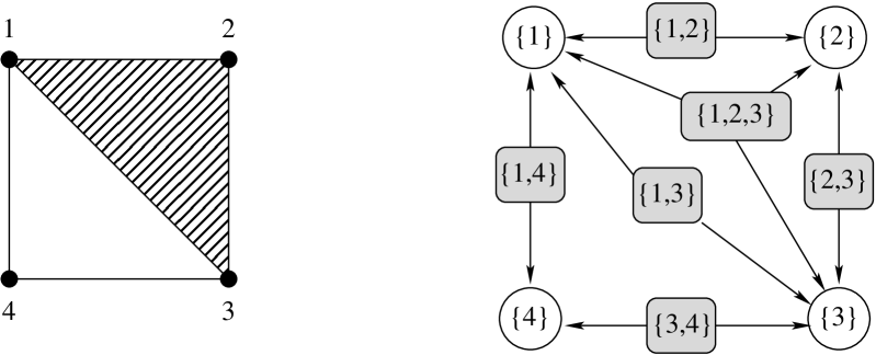
Here, we draw the digraph that has vertex set and
the edges for all pairs of an index and a face
with . Note that is bipartite with
respect to the partitioning , where
are the singleton faces and
was defined above. See Figure 1 for an example.
Figure 1. A simplicial complex (left) and the acyclic bipartite
digraph corresponding to it (right).
In the setup of Proposition 6.1, the random
variables are functions of the hidden variables , up to the
noise given by the . There is a dual construction in
which the hidden variables are functions of the observed variables.
Suppose that the random variables are mutually independent
and normally distributed as with
. Suppose further that ,
, are mutually independent random
variables that are also independent of the . Define
random variables as linear combinations:
(6.4)
Note that this equation system is associated with the bipartite
acyclic digraph obtained by reversing the direction of all edges in
.
Proposition 6.2.
If the random vector is
defined by (6.4), then the positive definite matrix
is the inverse of the covariance matrix of the
conditional distribution of given .
Proof.
Concatenating and yields a Gaussian random vector
with covariance matrix
where we have reused the matrices appearing in (6.2) and
(6.3). By standard results about
conditional distributions of Gaussian random vectors, the covariance
matrix of the conditional distribution of given is
the Schur complement
It follows from the matrix inversion lemma that the inverse of the
conditional covariance matrix is
According to Proposition 6.2, positive definite
matrices in also arise as inverses of conditional
covariance matrices. Zeros in the inverse of the covariance matrix of a
Gaussian random vector have an appealing interpretation in terms of
conditional independence; see again [DSS09, Chap. 3].
Acknowledgments
We thank Anton Leykin, Sonja Petrovic, Bernd Sturmfels, and Caroline
Uhler for helpful discussions and anonymous referees for detailed
comments and for suggesting a simpler alternative proof of Lemma
5.6, which we had previously proven by applying
Bernstein’s theorem. Josephine Yu was supported by an NSF
postdoctoral research fellowship. Mathias Drton was supported by the
NSF under Grant No. DMS-0746265 and by an Alfred P. Sloan Fellowship.
References
[AHMR88]
Jim Agler, J. William Helton, Scott McCullough, and Leiba Rodman,
Positive semidefinite matrices with a given sparsity pattern,
Proceedings of the Victoria Conference on Combinatorial Matrix
Analysis (Victoria, BC, 1987), vol. 107, 1988, pp. 101–149.
MR960140 (90h:15030)
[Bar08]
David Barber, Clique matrices for statistical graph decomposition and
parameterising restricted positive definite matrices, Proceedings of the
24th Conference in Uncertainty in Artificial Intelligence (David A.
McAllester and Petri Myllymäki, eds.), AUAI Press, 2008, pp. 26–33.
[CDS95]
Dragoš M. Cvetković, Michael Doob, and Horst Sachs, Spectra of
graphs, third ed., Johann Ambrosius Barth, Heidelberg, 1995, Theory and
applications. MR1324340 (96b:05108)
[CW96]
D. R. Cox and Nanny Wermuth, Multivariate dependencies, Monographs on
Statistics and Applied Probability, vol. 67, Chapman & Hall, London, 1996,
Models, analysis and interpretation. MR1456990 (98m:62003)
[DP07]
Mathias Drton and Michael D. Perlman, Multiple testing and error control
in Gaussian graphical model selection, Statist. Sci. 22 (2007),
no. 3, 430–449. MR2416818
[DSS09]
Mathias Drton, Bernd Sturmfels, and Seth Sullivant, Lectures on algebraic
statistics, Birkhäuser Verlag, Basel, Switzerland, 2009.
[HPR89]
J. W. Helton, S. Pierce, and L. Rodman, The ranks of extremal positive
semidefinite matrices with given sparsity pattern, SIAM J. Matrix Anal.
Appl. 10 (1989), no. 3, 407–423. MR1003106 (90j:05094)
[Lau01]
Monique Laurent, On the sparsity order of a graph and its deficiency in
chordality, Combinatorica 21 (2001), no. 4, 543–570. MR1863577
(2002i:05080)
[PDB07]
Jesus Palomo, David B. Dunson, and Ken Bollen, Bayesian structural
equation modeling, Handbook of Latent Variable and Related Models (Sik-Yum
Lee, ed.), Elsevier, Amsterdam, 2007, pp. 163–188.
[PPS89]
Vern I. Paulsen, Stephen C. Power, and Roger R. Smith, Schur products and
matrix completions, J. Funct. Anal. 85 (1989), no. 1, 151–178.
MR1005860 (90j:46051)
[RS02]
Thomas Richardson and Peter Spirtes, Ancestral graph Markov models,
Ann. Statist. 30 (2002), no. 4, 962–1030. MR1926166
(2003h:60017)
[SRM+98]
Peter Spirtes, Thomas Richardson, Christopher Meek, Richard Scheines, and Clark
Glymour, Using path diagrams as a structural equation modelling tool,
Sociological Methods and Research 27 (1998), 182–225.
[STD10]
Seth Sullivant, Kelli Talaska, and Jan Draisma, Trek separation for
Gaussian graphical models, Ann. Statist. 38 (2010), no. 3,
1665–1685.