Sidelobe Control in Collaborative Beamforming via Node Selection

Abstract

Collaborative beamforming (CB) is a power efficient method for data communications in wireless sensor networks (WSNs) which aims at increasing the transmission range in the network by radiating the power from a cluster of sensor nodes in the directions of the intended base station(s) or access point(s) (BSs/APs). The CB average beampattern expresses a deterministic behavior and can be used for characterizing/controling the transmission at intended direction(s), since the mainlobe of the CB beampattern is independent on the particular random node locations. However, the CB for a cluster formed by a limited number of collaborative nodes results in a sample beampattern with sidelobes that severely depend on the particular node locations. High level sidelobes can cause unacceptable interference when they occur at directions of unintended BSs/APs. Therefore, sidelobe control in CB has a potential to increase the network capacity and wireless channel availability by decreasing the interference. Traditional sidelobe control techniques are proposed for centralized antenna arrays and, therefore, are not suitable for WSNs. In this paper, we show that distributed, scalable, and low-complexity sidelobe control techniques suitable for CB in WSNs can be developed based on node selection technique which make use of the randomness of the node locations. A node selection algorithm with low-rate feedback is developed to search over different node combinations. The performance of the proposed algorithm is analyzed in terms of the average number of trials required to select the collaborative nodes and the resulting interference. Our simulation results approve the theoretical analysis and show that the interference is significantly reduced when node selection is used with CB.

I INTRODUCTION

Wireless sensor networks (WSNs) have become practical technology due to the production of low cost, low-power, and small size sensors. Different applications such as habitat and climate monitoring, detection of human/vehicular intrusion, and etc. are increasingly employing WSNs [1]. Such applications require sensor nodes to be deployed over a remote area to collect data from the surrounding environment and communicate it to far base stations or access points (BSs/APs). As a result, the challenges faced in the WSN applications are quite different from that of considered in the applications of the traditional wireless ad-hoc networks [2]. These differences can be summarized as follows.

• Typical WSN is densely deployed and may consist of thousands of sensor nodes.

• The network geometry changes all the time due to failure of sensor nodes or deployment of new sensor nodes.

• Sensor nodes are battery-powered and the battery often cannot be replaced. Thus, the sensor node life time is limited by the battery lifetime.

• Sensor nodes have simple hardware with limited computational capabilities and small memory in order to keep the production cost of the sensor node reasonable.

• Sensor nodes can fail easily. Thus, it is desired that the WSN performance does not depend on individual sensor nodes.

• Data and traffic models in WSNs depend on the application, and usually the data is redundant, while the traffic has low-rate burst nature.

• Sensor nodes in WSNs are usually deployed at the ground level and have no mobility. Thus, the channel path loss for individual node is high and the channel variations are slow.

Practical communication schemes for WSNs should overcome the problem of limited transmission range of individual sensor nodes, while being distributed and scalable. Moreover, for designing such communication schemes, power consumption and implementation complexity issues have to be taken into account as the most significant design constraints for WSNs.

To address the aforementioned issues, the inherent high density deployment of sensor nodes has been used to introduce collaborative beamforming (CB) for the uplink communication to a BS/AP [3], [4]. CB extends the transmission range of individual sensor nodes by using a cluster of sensor nodes in a power-efficient way. Particularly, sensor nodes from a cluster of nodes act collaboratively as distributed antenna array to form a beam toward the direction(s) of the intended BS(s)/AP(s). Given that each sensor node is equipped with a single omnidirectional antenna and operates in half-duplex mode, CB is performed in two stages. In the first stage, the data from source node(s) in a cluster is shared with all other collaborative nodes, while in the second stage, this data is transmitted by all sensor nodes simultaneously and coherently. In the latter stage, sensor nodes adjust the initial phase of their carriers so that the individual signals from different sensor nodes arrive in phase and constructively add at the intended BS/AP. In this way, CB is able to increase the area coverage of WSNs and, therefore, can be also viewed as an alternative scheme to the multi-hop relay communications. However, as compared to the multi-hop relay communications, CB brings the following advantages.

• For CB, there is no dependency of communication quality on individual nodes. Thus, the communication link is more reliable.

• CB distributes the power consumptions over large number of sensor nodes and balances the lifetimes of individual nodes [5].

• CB enables to create a direct single-hop uplink to the intended BS(s)/AP(s). Thus, it reduces the communication delay and data overhead.

• CB achieves higher connectivity than that of omnidirectional transmission with the same transmit power [6].

In order to implement CB, the following issues related to the the distributed nature of the WSNs have been addressed. Distributed schemes for estimating the initial phases of the local node oscillators in WSNs have been introduced in [7]–[9]. These schemes allow to achieve phase synchronization among all collaborative nodes in a cluster of WSN. Moreover, to minimize the time required for multiple sources to share the data among all sensor nodes in a cluster, a medium access control-physical (MAC-PHY) CB scheme which is based on the medium random access has been proposed in [10].

Although, the above mentioned implementation issues for CB have been positively addressed, one more concern is that the random sensor node locations result in a random beampattern which depends on the actual locations. The effect of the spatial sensor node distribution on the directivity of the CB beampattern has been studied in [3] (see also [11]) for the case of uniform sensor node distribution and in [4],[12], [13] for the case of Gaussian sensor node distribution. Although it has been shown for both aforementioned node distributions that the CB sample beampattern has a deterministic mainlobe which is independent on the random sensor node locations, the sidelobes of the CB sample beampattern are totaly random and can be described only in statistical terms [3], [4, 13]. In addition, the aforementioned multiple access scheme of [10], which minimizes the time required for sharing the multiple source data, results in higher sidelobes even for the average CB beampattern. All these can lead to high interference levels at the directions of unintended BSs/APs. Therefore, the sidelobe control problem arises in the context of WSNs. Indeed, achieving a sample CB beampattern with lower sidelobe interference at unintended BSs/APs has the potential to increase the WSN throughput [14].

Due to the inherent distributed nature of WSNs, the sidelobe control should be achieved with minimum data overhead and knowledge of the channel information. Unfortunately, traditional sidelobe control techniques [15, 17] cannot be applied in the context of WSNs due to their unacceptably high complexity and the requirement of centralized processing. Indeed, to apply the centralized beamforming weight design in the WSNs, a node or BS/AP has to collect the location and channel information from all sensor nodes. It can significantly increase the overhead in the network and nullify the above mentioned advantages of CB. Note that for the same reasons the recently developed network beamforming techniques [19, 21] are restricted to the applications in the relay networks only and it is impractical to apply them for WSNs.

In this paper, we develop a technique for sidelobe control in CB for WSNs which is based on sensor node selection. Such technique makes use of the randomness of node locations and is distributed and scalable as well as it has low data overhead. Moreover, as compared to the optimal beamforming weights assignment, our sidelobe control technique which is based on the phase synchronization and simple node selection is more robust to the channel/phase errors. In addition, it helps to balance the life times of all sensor nodes since the corresponding beamforming weights have the same magnitude for all nodes. For the sidelobe control technique, a node selection algorithm with low-rate feedback is developed to search over different node combinations. The performance of the proposed algorithm is analyzed in terms of the average number of trials required to select the collaborative nodes and the distribution of the resulting interference.

The paper is organized as follows. System and signal models are introduced in Section II. A new sidelobe control technique for CB in WSNs is developed in Section III where the node selection algorithm is also summarized. The performance characteristics of the proposed node selection algorithm such as the average number of trials required to select the collaborative nodes and the resulting interference are studied in Section IV. Section V reports our simulation results and is followed by conclusions in Section VI. Proofs of some results in the paper are summarized in Appendixes.

II SYSTEM AND SIGNAL MODEL

II-A System Model

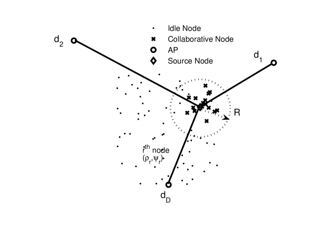
Figure 1: WSN model with multiple BSs/APs.

We consider a WSN with nodes randomly placed over a plane as shown in Fig. 1. Multiple BSs/APs, denoted as ${\cal D}=\{d_{0},d_{1},d_{2},\dots,d_{D}\}$, are located outside and far apart from the coverage area of each individual node at directions $\varphi_{0},\varphi_{1},\varphi_{2},\dots,\varphi_{D}$, respectively. Uplink transmission is a burst traffic for which the nodes are idle most of the time and have sudden transmissions. Thus, we adopt a time-slotted scheme where nodes are allowed to transmit at the beginning of each time slot. The downlink transmissions are mostly the control data broadcasted over a separate error-free control channels. The BSs/APs can use high power transmission and, therefore, the downlink is less challenging and can be organized as direct transmission.

We assume that due to the limited power of individual nodes, direct transmission to the BSs/APs is not feasible and sensor nodes have to employ CB for the uplink transmission. The distance between nodes in one cluster of WSN is small so that the power consumed for communication among nodes in the cluster can be neglected. Each sensor node is equipped with a single antenna used for both transmission and reception. To identify different nodes and BSs/APs, each node or BS/AP to has a unique identification (ID) sequence that is included in each transmission.

At each time slot, a set ${\cal S}=\{s_{0},s_{1},s_{2},\dots,s_{S}\}$ of source nodes is active. Moreover, only $K$ source–destination pairs are allowed to communicate. Here $K=\min\{{\rm card}(\cal S),{\rm card}(\cal D)\}$ where ${\rm card}(\cdot)$ denotes the cardinality of a set, and the $k$th source–destination pair is denoted as $s_{k}$–$d_{k}$. For source node $s_{k}$, the coverage area is, ideally, a circle with a radius which depends on the power allocated for the node-to-node communication.

Let ${\cal M}^{k}$ be a set of nodes in the coverage area of the node $s_{k}$. Let us, therefore, select the source node $s_{k}$ as a local origin of the coordinate system used to mark the spatial locations of the nodes in the coverage area of $s_{k}$, i.e. ${\cal M}^{k}$. The $r$th collaborative node, denoted as $c_{r}$, $r\in{\cal M}^{k}$, has a polar coordinates $\left(\rho_{r},\psi_{r}\right)$. The Euclidean distance between the collaborative node $c_{r}$ and a point $(A,\phi)$ in the same plane is defined as

$$d_{r}(\phi)\triangleq\sqrt{{A}^{2}+\rho_{r}^{2}-2\rho_{r}{A}\cos(\phi-\psi_{k})}\approx A-\rho_{r}\cos(\phi-\psi_{r})$$ (1)

where $A\gg r_{k}$ in the far-field region.

The array factor for the set of sensor nodes ${\cal M}^{k}$ in a plane can be defined as

$$AF_{k}(\phi)=\sum_{r\in{\cal M}^{k}}\sqrt{P_{r}}e^{j\theta_{r}^{k}}e^{-j\theta_{r}(\phi)}$$ (2)

where $P_{r}$ is the transmission power assigned to each node, $\theta_{r}^{k}$ is the initial phase of the $r$th sensor carrier frequency, $\theta_{r}(\phi)=\frac{2\pi}{\lambda}d_{r}(\phi)$ is the phase delay due to propagation at the point $(A,\phi)$, and $\lambda$ is the wavelength. Then the far-field beampattern corresponding to the set of sensor nodes ${\cal M}^{k}$ can be found as

$$BP_{k}(\phi)\triangleq\left|AF_{k}(\phi)\right|^{2}=\left|\sum_{r\in{\cal M}^{k}}\sqrt{P_{r}}e^{j\theta_{r}^{k}}e^{-j\theta_{r}(\phi)}\right|^{2}$$ (3)

where $|\cdot|^{2}$ denotes the magnitude of a complex number.

It is assumed that the symbol duration is very short as compared to the channel coherent time. Therefore, the channel variations can be considered to be quasi-static during one symbol transmission. Since sensor nodes are located at the ground level, the large-scale fading is the dominant factor for the channels between collaborative nodes in ${\cal M}^{k}$ and BSs/APs. Then the channel coefficient for $r$th collaborative node which serves $k$th source–destination pair can be modeled as

$$h_{rk}=a_{rk}b_{rk}$$ (4)

where $b_{rk}$ is the attenuation/path loss factor in the channel coefficient due to propagation distance and $a_{rk}$ is a lognormal distributed random variable which represents the flactuation/shadowing effect in the channel coefficient, i.e., $a_{rk}\sim\exp\{{\cal N}(m,\sigma^{2})\}$. Here $m$ and $\sigma^{2}$ denote respectively the mean and variance, of the corresponding Gaussian distribution. Then the mean and variance of the lognormally distributed $a_{rk}$ can be found as

$$m_{a_{rk}}\!\! = \!\!E\left\{a_{rk}\right\}=e^{m+{\frac{\sigma^{2}}{2}}}$$ (5)

$$\sigma_{a_{rk}}^{2}\!\! = \!\!E\left\{a_{rk}^{2}\right\}=\left(e^{\sigma^{2}}-1\right)\left(e^{2m+\sigma^{2}}\right)$$ (6)

where $E\{\cdot\}$ stands for the statistical expectation. The attenuation/path loss depends on the distance between $c_{r}$ and $d_{k}$ and the path loss exponent. Assuming that all nodes in ${\cal M}^{k}$ are close to each other, the pass losses from the nodes in ${\cal M}^{k}$ to the BS/AP are equal to each other, i.e., $b_{rk}=b_{k}$, $r\in{\cal M}^{k}$ [22]. Moreover, since all BSs/APs are located far apart from the cluster of collaborative nodes, the network can be viewed as homogeneous and the attenuation effects of different paths can be assumed approximately equal to each other, i.e., $b_{k}=b$ [23]. Note that even if the attenuation effects for different BSs/APs are different, they can be compensated by adjusting the gains of the corresponding receivers or the power/number of the corresponding collaborative nodes participating in CB.

II-B CB and Corresponding Signal Model

Consider a two–step transmission which consists of the information sharing and the actual CB steps. Information sharing aims at broadcasting the data from one source node to all other nodes in its coverage area. Specifically, in this step, the source node $s_{k}$ broadcasts the data symbol $z_{k}$ to all nodes in its coverage area ${\cal M}^{k}$, where the data symbol $z_{k}\in{\mathbb{C}}$ belongs to a codebook of zero mean, unit power, and independent symbols, i.e., $E\left\{z_{k}\right\}=0$, $\left|z_{k}^{2}\right|=1$, and $E\left\{z_{k}z_{n}\right\}=0$ for $n\neq k$.

In the case of multiple source nodes sharing their own data with other nodes in their corresponding collaborative sets of nodes, a collision can occur. To avoid the collision, orthogonal channels in frequency, time, or code can be used. However, such collision avoidance causes resource loss and can lead to the network throughput reduction, especially if the number of source nodes sharing the data is large. Therefore, collision resolution schemes can be used alternatively (see for example [24], [25]). In this case, the information sharing takes only one time slot in a random access fashion. Finally, we assume that the power used for broadcasting the data by the source node is high enough so that each collaborative node $c_{r}$ can successfully decode the received symbol from the source node $s_{k}$.

During the CB step, each collaborative node $c_{r},r\in{\cal M}^{k}$, is first synchronized with the initial phase $\theta_{r}^{k}=-\frac{2\pi}{\lambda}\rho_{r}\cos(\varphi_{k}-\psi_{r})$ using the knowledge of the node locations (see the closed-loop scenario in [3]). Alternatively the synchronization can be performed without any knowledge of the node locations (see [7]–[9]). For example, the synchronization algorithm of [7] uses a simple 1-bit feedback iterations, while the methods of [8] and [9] are based on the time-slotted round-trip carrier synchronization approach.

After synchronization, all collaborative nodes transmit the signal coherently

$$t_{r}=z_{k}e^{j\theta_{r}^{k}},\quad r\in{\cal M}^{k}.$$ (7)

Then the received signal at angle $\phi$ can be given as

$$g(\phi)=\sum_{k}z_{k}\sum_{r\in{\cal M}^{k}}\sqrt{P_{r}}a_{rk}e^{j\theta_{r}^{k}}e^{-j\theta_{r}(\phi)}+w$$ (8)

where $w\sim{\cal CN}(0,\sigma_{w}^{2})$ is the additive white Gaussian noise (AWGN) at the direction $\phi$. Note that the white noise is the same at all angles and, therefore, it disturbs the CB beampattern (3) equally in all directions. The received noise power $\sigma_{w}^{2}$ at BSs/APs can be measured in the absence of data transmission and, therefore, is assumed to be known at each BS/AP.

The received signal at the intended BS/AP $d_{k^{*}}$ can be written as

$$g_{k^{*}}\triangleq g(\varphi_{k^{*}}) = z_{k^{*}}\sum_{r\in{\cal M}^{k^{*}}}\sqrt{P_{r}}a_{r{k^{*}}}+\sum_{k\neq k^{*}}z_{k}\sum_{r\in{\cal M}^{k}}\sqrt{P_{r}}a_{r{k^{*}}}e^{-j(\theta_{r}^{k^{*}}-\theta_{r}^{k})}+w$$ (9)

$$= z_{k^{*}}\sum_{r\in{\cal M}^{k^{*}}}\sqrt{P_{r}}a_{r{k^{*}}}+\sum_{k\neq k^{*}}z_{k}\sum_{r\in{\cal M}^{k}}\sqrt{P_{r}}a_{r{k^{*}}}\left(x_{r}^{(k^{*},k)}-jy_{r}^{(k^{*},k)}\right)+w$$

where $x_{r}^{(k^{*},k)}={\cal R}\left\{e^{-j(\theta_{r}^{k^{*}}-\theta_{r}^{k})}\right\}$, $y_{r}^{(k^{*},k)}={\cal I}\left\{e^{-j(\theta_{r}^{k^{*}}-\theta_{r}^{k})}\right\}$ and ${\cal R}\left\{\cdot\right\}$ and ${\cal I}\left\{\cdot\right\}$ represent the real and the imaginary parts of a complex number, respectively. Note that $x_{r}^{(k^{*},k)}$ and $y_{r}^{(k^{*},k)}$ are random variables. It can be further shown (see Appendix A) that $u\in\left\{x_{r}^{(k^{*},k)},y_{r}^{(k^{*},k)}\right\}$ has mean $m_{x_{r}^{(k^{*},k)}}=m_{y_{r}^{(k^{*},k)}}=m_{u}=E\left\{u\right\}=0$ and variance $\sigma_{x_{r}^{(k^{*},k)}}^{2}=\sigma_{y_{r}^{(k^{*},k)}}^{2}=\sigma_{u}^{2}=E\left\{u^{2}\right\}=0.5$. The first term in (9) is the signal received at the the BS/AP $d_{k^{*}}$ from the desired set of collaborative nodes ${\cal M}^{k^{*}}$, while the second term represents the interference caused by other sets of nodes ${\cal M}^{k}$, $k\neq k^{*}$ where ${\cal M}^{k}\cap{\cal M}^{n}=\varnothing$, $k\neq n$. Assumed that each node in the network utilizes the same amount of power for each CB transmission, i.e., $P_{r}=P$, the received signal (9) at the BS/AP $d_{k^{*}}$ can be rewritten as

$$g_{k^{*}}=\sqrt{P}\ \ z_{k^{*}}\sum_{r\in{\cal M}^{k^{*}}}a_{r{k^{*}}}+\sqrt{P}\sum_{k\neq k^{*}}z_{k}\sum_{r\in{\cal M}^{k}}a_{r{k^{*}}}\left(x_{r}^{(k^{*},k)}-jy_{r}^{(k^{*},k)}\right)+w.$$ (10)

III Sidelobe Control via Node Selection

In dense WSNs, each source node is surrounded by many candidate collaborative nodes in its coverage area. Although it has been shown earlier that the sidelobe levels of the average beampattern decrease inverse proportionally and uniformly over all directions with the increase of the number of collaborative nodes [3], [4], the sidelobe levels at particular directions of interest (unintended BSs/APs) in the sample beampattern are totaly random and can be unacceptably high if the number of collaborative nodes is not very large. At the same time, the randomness of the node locations provides additional degrees of freedom for controlling the beampattern sidelobes. Indeed, the sidelobes corresponding to different sets of collaborative nodes are different [3], [4].

The problem of high sidelobe levels at specific directions for the average beampattern has been briefly discussed in [26]. It is suggested there to use only the sensor nodes placed in multiple concentric rings instead of using all nodes in the disk of the coverage area. However, a narrower ring with larger radiuses results in the average beampattern with smaller mainlobe width and leads to larger sidelobe peak levels at other uncontrolled directions than the conventional CB. Moreover, only the average beampattern behavior is considered in [26], while it is the sample beampattern behavior that is of real importance for the sidelobe control in WSNs.

Exploiting the randomness of the node locations in WSNs, we introduce and study in this section a node selection algorithm for sidelobe control of the CB sample beampattern as a method for interference reduction. A sidelobe control approach based on node selection is suitable for WSN applications because it allows to avoid complex central beamforming weight design and corresponding additional communications.

It is required to select a subset of collaborative nodes from the candidate nodes in the coverage area of the source node. Let ${\cal N}^{k}$ be a set of collaborative nodes to be selected from ${\cal M}^{k}$, i.e., ${\cal N}^{k}\subset{\cal M}^{k}$, to beamform data symbols to $d_{k}$. Note that in accordance with [3] and [4], the mainlobe of the beampattern is stable and does not change for different subsets of ${\cal M}^{k}$ as long as the the size of the coverage area does not change and the WSN is sufficiently dense, i.e., each cluster of the WSN consists of a sufficiently large number of sensor nodes. Also note that the set ${\cal N}^{k}$ can be updated any time when the channel conditions or network configuration change. Alternatively, it can be updated periodically to balance power consumptions among nodes. The meaningful objective for node selection is to achieve a beampattern with low level sidelobes toward the unintended BS/AP directions.

Toward this end, we develop a low-complexity distributed node selection algorithm, which guarantees that the sidelobe levels toward unintended direction(s) are below a certain prescribed value(s) as long as the WSN is sufficiently dense. An algorithm utilizes only the knowledge of the received interference power to noise ratio (INR), denoted as $\eta$, at the unintended destinations and requires only low-rate (essentiality, one-bit) feedback from the unintended BSs/APs at each trial. Although our node selection strategy does not guarantee the optimum result of centralized beamforming strategies (which require global CSI and, therefore, a very significant data overhead in the network), it has the following practically important advantages for applying in the WSNs context.

• It is very simple computationally and can be run in cheap sensor nodes without adding any computations.

• It has a distributed nature and, therefore, uses minimum control feedback from the unintended BSs/APs.

In the following, we first describe the communication protocol and then give the details of the node selection algorithm.

III-A Communication Protocol

Data transmission is organized in the following steps.

• At the beginning of each time-slot, the source node $s_{k}$ listens to the control channels from BSs/APs and checks for an available BS/AP.

• The source node $s_{k}$ broadcasts its ID and the ID of the available BS/AP $d_{k}$ to the nodes in its coverage area ${\cal M}^{k}$. Note that all transmissions from the source node $s_{k}$ to the intended destination $d_{k}$ will be achieved through the CB using the nodes in the set of collaborative nodes ${\cal N}^{k}\subset{\cal M}^{k}$.

• The source node $s_{k}$ attempts to transmit its ID to the target BS/AP. If a collision occurs, i.e., if the target BS/AP receives transmissions form more than one collaborative sets of sensor nodes, the BS/AP approves only one set of nodes for data transmission.

• At the beginning of each following time-slot, the BS/AP broadcasts through the control channels the selected source ID in addition to one bit of information which indicates that the BS/AP is busy. In this case, other source nodes are not allowed to transmit data to the same BS/AP.

• Finally, only the predetermined subset of collaborative nodes ${\cal N}^{k}$ assigned to the pair $s_{k}$–$d_{k}$ continues to receive data, while other nodes go back to idle mode, that is, the actual data transmission takes a place for the pair $s_{k}$–$d_{k}$.

III-B Node Selection Algorithm

A set of collaborative nodes ${\cal N}^{k}\subset{\cal M}^{k}$ is assigned to each source–distention pair $s_{k}$–$d_{k}$. To select such a collaborative set, the nodes can be tested one by one or a group of nodes by a group of nodes. The latter is, however, preferable since it can significantly reduce the data overhead in the system. Indeed, while testing one node or a group of nodes, we need to check if the corresponding CB beampattern sidelobe level reduces in the unintended direction(s) and then send the ‘approve/reject’ bit per one node in the fist case, or per a group of nodes in the second case. Therefore, if every group of nodes consists of a larger number of sensor nodes, less ‘approve/reject’ bits has to be sent in the system in total.

Consider the source node $s_{k^{*}}$, let the number of nodes in its coverage area is $M$, the number of collaborative nodes needed to be selected is $N\leq M$, and the size of one group of nodes to be tested in each trial is $L\leq N$. Using the selection principle highlighted above, the selection process can be organized in the following two steps.

• Selection. Source node $s_{k^{*}}$ initiates the node selection by broadcasting the select message to the nodes in its coverage area, namely the set ${\cal M}^{k^{*}}$, and randomly selects a subset ${\cal L}^{k^{*}}$ of $L$ candidate nodes from ${\cal M}^{k^{*}}$.

  The nodes can be assigned to the set ${\cal L}^{k^{*}}$ by using any of the following two methods. The first one is a centralized method in which the source node $s_{k^{*}}$ is totally responsible for the node assignment. According to this method, every source node maintains a table of IDs of all candidate nodes in its coverage area and randomly assigns nodes to the set ${\cal L}^{k^{*}}$. The source node $s_{k^{*}}$ then broadcasts the IDs of the nodes assigned to the set ${\cal L}^{k^{*}}$ to inform them that they are selected for the test. The disadvantage of this method is that it is suitable only for small WSNs where each source node can keep records of all other nodes in its coverage area. As a result, this method typically requires large data exchange between the source and the candidate nodes.

  Alternatively, in the second method, node assignment task is distributed among the source and collaborative nodes. In particular, if collaborative nodes receive the select message, each node starts a random delay using an internal timer. After the random delay, the candidate node responds by the offer message which contains the ID of this node. Then the source node responds by the approval message which requires only 1 bit of feedback. If a collision occurs and two collaborative nodes transmit the offer message at the same time, the source node responds by the approval message with a different bit value and the timers in both nodes start over a new random delay. The process repeats and the source node $s_{k^{*}}$ keeps sending the select message until $L$ candidate nodes are assigned and the set ${\cal L}^{k^{*}}$ is constructed.

• Test. The set ${\cal L}^{k^{*}}$ transmits the test message that contains the intended BS/AP ID to the intended destination $d_{k^{*}}$ using CB. While the intended destination $d_{k^{*}}$ receives a predetermined signal power level, the interference power levels at the unintended destination(s) $d_{k}$, $k\neq k^{*}$ are random because of the random sidelobes of the CB beampattern. At this stage, all unintended BSs/APs with different IDs measure the received INR $\eta$. If $\eta$ is higher than a predetermined threshold value $\eta_{\text{thr}}$, the reject message is sent back to the candidate set ${\cal L}^{k^{*}}\!\!\!$. In this case, the nodes in the candidate set ${\cal L}^{k^{*}}$ are all returned to the set of nodes ${\cal M}^{k^{*}}$ and can be used in future trials. If no reject message is received from any of the unintended BSs/APs after a predetermined time, then the candidate set ${\cal L}^{k^{*}}$ is approved and each node from the candidate set ${\cal L}^{k^{*}}$ stores the IDs of the source node $s_{k^{*}}$ and the destination $d_{k^{*}}$. Then the collaborative nodes assigned to serve the pair $s_{k^{*}}$–$d_{k^{*}}$ do not participate in future trials. In this way, we can avoid an overlap between sets of nodes serving different BSs/APs.

  In order to select $N$ collaborative nodes, the Selection and Test steps are repeated until $N/L$ candidate sets ${\cal L}_{l}^{k^{*}}$, $l=1,2,\dots,N/L$, are approved. Then the so obtained set of approved collaborative nodes is ${\cal N}^{k^{*}}=\bigcup_{l}{\cal L}_{l}^{k^{*}}$.

  Once $N$ nodes are selected, i.e., ${\cal N}^{k^{*}}$ is constructed, the source node $s_{k^{*}}$ broadcasts the end message and no more candidate sets ${\cal L}^{k^{*}}$ is constructed.

The pseudocode of the node selection algorithm is given in Table I.

Node selection algorithm

Initial values:

$N$ and $L$ are predetermined at the Source Node $s_{k^{*}}$.

$\eta_{\text{thr}}$ is predetermined at the unintended Destinations $d_{k}$, $k=\{0,1,\dots,D\}$.

1: At $s_{k^{*}}$: ($\text{Counter }{l}\leftarrow 1$).

2: If ($\text{Counter }{l}<\frac{N}{L}$),

3:        Then: { $s_{k^{*}}$ broadcasts the select message.

4:                   A candidate set ${\cal L}_{l}^{k^{*}}$ is constructed.

5:                   Using CB, the nodes in ${\cal L}_{l}^{k^{*}}$ transmit the test message.}

6:         Otherwise: {Go to 12.}

7: At any $d_{k}$, $k\neq k^{*}$: If ( The received INR $\eta>\eta_{\text{thr}}$),

8:         Then { $d_{k}$ sends the reject message to ${\cal L}_{l}^{k^{*}}$.}

9:         Else   { No reject message is received.

10:                  ${\cal L}_{l}^{k^{*}}$ is approved and the corresponding nodes store the IDs of $s_{k^{*}}$ and $d_{k^{*}}$.

11:                 At $s_{k^{*}}$: ($\text{Counter }{l}\leftarrow\text{Counter }{l+1}$). Go to 2.}

12: $s_{k^{*}}$ broadcasts the end message.

TABLE I: Table 1: Node selection algorithm for CB sidelobe control.

IV Performance Analysis

In this section, we analyze the proposed node selection algorithm in terms of (i) the average number of trials required for selecting a set of collaborative nodes which guarantee low interference level for unintended BSs/APs and (ii) the complementary cumulative distribution function (CCDF) of the INR $\eta$. The first characteristic allows to estimate the average run time of the algorithm, while the second characteristic is needed to estimate the achievable interference levels versus the corresponding interference threshold values.

IV-A The Average Number of Trials

Note that the signal-to-noise ratio (SNR), denoted as $\gamma$, received through the link $s_{k^{*}}$–$d_{k^{*}}$ at the intended BS/AP should be above a certain level which guarantees the correct detection with high probability. This SNR at the intended BS/AP must be guaranteed regardless of the number of collaborative nodes participating in the CB. Therefore, we assume in our analysis that the total transmit power budget for each tested candidate set of nodes is kept the same in each trial of CB transmission. In particular, if the SNR at the intended BS/AP is required to be $10\log_{10}(\gamma)$ dB, then in the selection process, the power per one sensor node in ${\cal L}_{l}^{k^{*}}$ has to be set as $P=\sigma_{w}^{2}\gamma/L\leq P^{\rm max}$, where $P^{\rm max}$ is the maximum available power at the node. Also note that the power consumed for running the node selection algorithm is, in fact, proportional to the average number of trials in the algorithm. Therefore, it is preferable to construct a set of collaborative nodes with less number of trials.

In order to derive the average number of trials for the node selection algorithm, we, first, need to find the probability that a candidate set of nodes ${\cal L}_{l}^{k^{*}}$ is approved as part of the set of collaborative nodes ${\cal N}^{k^{*}}$. This probability is the same as the probability that the set ${\cal L}_{l}^{k^{*}}$ generates an acceptable interference at the unintended BSs/APs. Since we assumed that only one set of collaborative nodes ${\cal N}^{k^{*}}$ is constructed at a time, there is no interference present from other collaborative sets. Therefore, the interference power received at the unintended BS/AP $d_{k}$ from the tested candidate set of nodes ${\cal L}_{l}^{k^{*}}$ which targets the intended BS/AP $d_{k^{*}}$ can be written as

$$I\left(\varphi_{k}\left|{\cal L}_{l}^{k^{*}}\right.\right)=\sqrt{\frac{\sigma_{w}^{2}\gamma}{L}}z_{k^{*}}\!\!\sum_{r\in{\cal L}_{l}^{k^{*}}}a_{rk}\left(x_{r}^{(k^{*},k)}-jy_{r}^{(k^{*},k)}\right)$$ (11)

where $z_{k^{*}}$, $a_{rk}$, $x_{r}^{(k^{*},k)}$, and $y_{r}^{(k^{*},k)}$ are defined in Section II.

Equivalently, (11) can be rewritten as

$$I\left(\varphi_{k}\left|{\cal L}_{l}^{k^{*}}\right.\right)\!\! = \!\!\sqrt{\frac{\sigma_{w}^{2}\gamma}{L}}z_{k^{*}}\!\!\sum_{r\in{\cal L}_{l}^{k^{*}}}\left({x^{\prime}}_{r}^{(k^{*},k)}-j{y^{\prime}}_{r}^{(k^{*},k)}\right)$$ (12)

$$= \!\!z_{k^{*}}\left(\sqrt{\frac{\sigma_{w}^{2}\gamma}{L}}\!\!\sum_{r\in{\cal L}_{l}^{k^{*}}}{x^{\prime}}_{r}^{(k^{*},k)}-j\sqrt{\frac{\sigma_{w}^{2}\gamma}{L}}\!\!\sum_{r\in{\cal L}_{l}^{k^{*}}}{y^{\prime}}_{r}^{(k^{*},k)}\right)$$

where ${x^{\prime}}_{r}^{(k^{*},k)}\triangleq a_{rk}x_{r}^{(k^{*},k)}$ and ${y^{\prime}}_{r}^{(k^{*},k)}\triangleq a_{rk}y_{r}^{(k^{*},k)}$ with mean and variance given as

$$m_{1}\!\! = \!\!m_{a_{rk}}m_{u}=0,$$ (13)

$$\sigma_{1}^{2}\!\! = \!\!\left(\sigma_{u}^{2}+m_{u}^{2}\right)\left(\sigma_{a_{rk}}^{2}+m_{a_{rk}}^{2}\right)-m_{a_{rk}}^{2}m_{u}^{2}=\sigma_{u}^{2}\sigma_{a_{rk}}^{2}.$$ (14)

Let us introduce the notations $X_{l}^{(k^{*},k)}\triangleq\sqrt{\sigma_{w}^{2}\gamma/L}\sum_{r\in{\cal L}_{l}^{k^{*}}}{x^{\prime}}_{r}^{(k^{*},k)}$ and $Y_{l}^{(k^{*},k)}\triangleq\sqrt{\sigma_{w}^{2}\gamma/L}$ $\times\sum_{r\in{\cal L}_{l}^{k^{*}}}{y^{\prime}}_{r}^{(k^{*},k)}$. Then $X_{l}^{(k^{*},k)}$ and $Y_{l}^{(k^{*},k)}$ can be approximated by Gaussian random variables [3, 11] with mean $m_{X}=m_{Y}=m_{1}=0$ and variance $\sigma_{X}^{2}=\sigma_{Y}^{2}=\gamma\sigma_{w}^{2}\sigma_{1}^{2}$. Thus, (12) can be finally rewritten as

$$I\left(\varphi_{k}\left|{\cal L}_{l}^{k^{*}}\right.\right)=z_{k^{*}}\left(X_{l}^{(k^{*},k)}-jY_{l}^{(k^{*},k)}\right).$$ (15)

Using (15) and the fact that $|z_{k^{*}}|^{2}=1$, the received interference power at the unintended BS/AP $d_{k}$ from the candidate set of nodes ${\cal L}_{l}^{k^{*}}$ can be expressed as

$$\left|I\left(\varphi_{k}\left|{\cal L}_{l}^{k^{*}}\right.\right)\right|^{2}=\left({X_{l}^{(k^{*},k)}}\right)^{2}+\left({Y_{l}^{(k^{*},k)}}\right)^{2}.$$ (16)

The probability that the candidate set of nodes ${\cal L}_{l}^{k^{*}}$ is approved to join the set of collaborative nodes ${\cal N}^{k^{*}}$, i.e, the probability that the INR $\eta$ from ${\cal L}_{l}^{k^{*}}$ at the unintended BS/AP $d_{k}$ is lower than the threshold value $\eta_{\text{thr}}$, can be then found as

$${\bf Pr}\left(\eta<\eta_{\text{thr}}\right)\!\! = \!\!{\bf Pr}\left(\frac{\left|I(\varphi_{k}\left|{\cal L}_{l}^{k^{*}}\right.)\right|^{2}}{\sigma_{w}^{2}}<\eta_{\text{thr}}\right)={\bf Pr}\left(\frac{\left({X_{l}^{(k^{*},k)}}\right)^{2}+\left({Y_{l}^{(k^{*},k)}}\right)^{2}}{\sigma_{w}^{2}}<\eta_{\text{thr}}\right)$$ (17)

$$= \!\!1-\exp\left(-\frac{\eta_{\text{thr}}\sigma_{w}^{2}}{2\sigma_{X}^{2}}\right)\triangleq p^{\prime}$$

where the INR $\eta=\left.\left\{\left({X_{l}^{(k^{*},k)}}\right)^{2}+\left({Y_{l}^{(k^{*},k)}}\right)^{2}\right\}\right/\sigma_{w}^{2}$ is exponentially distributed random variable with the probability density function (pdf)

$$f\left(\eta\ |\ \frac{\sigma_{w}^{2}}{2\sigma_{X}^{2}}\right)=\left\{\begin{matrix}\frac{\sigma_{w}^{2}}{2\sigma_{X}^{2}}\exp\left\{-\frac{\sigma_{w}^{2}\eta}{2\sigma_{X}^{2}}\right\},&\;\eta\geq 0\\ 0,&\;\eta<0\end{matrix}\right..$$ (18)

If $D$ unintended BSs/APs are present in the neighborhood of the set of candidate collaborative nodes ${\cal L}_{l}^{k^{*}}$, the probability that the INR from ${\cal L}_{l}^{k^{*}}$ at any one of these unintended BSs/APs is lower than the threshold value $\eta_{\text{thr}}$ is given by (17). Therefore, the probability that ${\cal L}_{l}^{k^{*}}$ is approved by all BSs/APs is the product of the probabilities that ${\cal L}_{l}^{k^{*}}$ is approved by each of the unintended BSs/APs, that is,

$$p=\left(1-\exp\left(-\frac{\eta_{\text{thr}}\sigma_{w}^{2}}{2\sigma_{X}^{2}}\right)\right)^{D}.$$ (19)

It can be seen from (19) that $p$ decreases if the threshold $\eta_{\text{thr}}$ decreases or the number $D$ of neighboring BSs/APs increases.

Using (19), a closed-form expression for the average number of trials required by the node selection algorithm can be derived. Note that the actual number of trials is a random variable which we will denote as $T$. In order to construct the set of collaborative nodes ${\cal N}^{k^{*}}$, $T_{0}=N/L$ trials must be successful among all $T$ trials. Since the candidate nodes are selected randomly at each trial of the node selection algorithm, the algorithm itself can be viewed as a sequence of Bernoulli trials. Since $T_{0}$ of these Bernoulli trials must be successful in order to construct ${\cal N}^{k^{*}}\!\!\!$, the probability distribution of $T$ in a sequence of Bernoulli trials is, in fact, negative binomial distribution, that is,

$${\bf Pr}(T=t)=\binom{t-1}{T_{0}-1}p^{T_{0}}\left(1-p\right)^{t-T_{0}}.$$ (20)

Using (20), the average number of trials for the proposed node selection algorithm can be obtained as (see the details of the derivation in Appendix B)

$$E\left\{T\right\}=\frac{T_{0}}{p}=\frac{N}{L\cdot p}.$$ (21)

It can be seen from (21) that the average number of trials is proportional to the size of the set of collaborative nodes ${\cal N}^{k^{*}}\!\!\!$, but it is inverse proportional to the size of the candidate set of nodes ${\cal L}_{l}^{k^{*}}$ and to the probability that the set ${\cal L}_{l}^{k^{*}}$ is approved to join the set ${\cal N}^{k^{*}}$. Therefore, less number of trials is required in average for the proposed node selection algorithm if $L$ is chosen to be large or $N$ is small. Moreover, if the probability $p$, which, in turns, depends on the threshold value $\eta_{\text{thr}}$ of the INR allowed at the unintended BSs/APs from the set ${\cal L}_{l}^{k^{*}}$ (see (19)), is large, then less number of trials is required.

IV-B The Complementary Cumulative Distribution Function of the Interference

Let us assume that $K(\leq D)$ collaborative sets are active and target different destination from $d_{k^{*}}$, these sets are ${\cal N}^{k}$, $k\neq k^{*}$, and their union is denoted hereafter as $\bigcup{\cal N}^{k\neq k^{*}}$. It can be seen from (10) that the total interference collected at the destination $d_{k^{*}}$ from these $K$ collaborative sets is

$$I\left(\varphi_{k^{*}}\,\left|\,\bigcup{\cal N}^{k\neq k^{*}}\right.\right)=\sqrt{\frac{\sigma_{w}^{2}\gamma}{N}}\sum_{k\neq k^{*}}z_{k}\sum_{r\in{\cal N}^{k}}a_{{k^{*}}r}\left(x_{r}^{(k^{*},k)}-jy_{r}^{(k^{*},k)}\right)$$ (22)

where the power per one collaborative sensor node is $P=\sigma_{w}^{2}\gamma/N$ because the SNR at the intended BS/AP must be $10\log_{10}(\gamma)$ dB. Using the fact that ${\cal N}^{k}=\bigcup{\cal L}_{l}^{k}$ and multiplying and dividing the right hand side of (22) by $\sqrt{L}$, the total interference at $d_{k^{*}}$ can be expressed as

$$I\left(\varphi_{k^{*}}\,\left|\,\bigcup{\cal N}^{k\neq k^{*}}\right.\right)\!\! = \!\!\sqrt{\frac{L}{N}}\sum_{k\neq k^{*}}z_{k}\sum_{l=1}^{N/L}\sum_{r\in{\cal L}_{l}^{k}}\sqrt{\frac{\sigma_{w}^{2}\gamma}{L}}\left({x^{\prime}}_{r}^{(k^{*},k)}-j{y^{\prime}}_{r}^{(k^{*},k)}\right)$$ (23)

$$= \!\!\sqrt{\frac{L}{N}}\sum_{k\neq k^{*}}z_{k}\sum_{l=1}^{N/L}\left(\tilde{X}_{l}^{(k^{*},k)}-j\ \tilde{Y}_{l}^{(k^{*},k)}\right)$$

where $\tilde{X}_{l}^{(k^{*},k)}$ and $\tilde{Y}_{l}^{(k^{*},k)}$ are zero mean truncated Gaussian distributed random variables corresponding to $X_{l}^{(k^{*},k)}$ and $Y_{l}^{(k^{*},k)}$ of (15) for only the approved candidate subsets. It can be shown that the marginal conditional probability density function of $\tilde{U}_{l}^{(k^{*},k)}\in\left\{\tilde{X}_{l}^{(k^{*},k)},\tilde{Y}_{l}^{(k^{*},k)}\right\}$ is [27]

$$\!\!f\left(\left.\tilde{U}_{l}^{(k^{*},k)}\,\right|\,\eta\leq\ \eta_{\text{thr}}\right)\!=\!f\left(\tilde{U}_{l}^{(k^{*},k)}\,\left|\,\left(\tilde{X}_{l}^{(k^{*},k)}\right)^{2}+\left(\tilde{Y}_{l}^{(k^{*},k)}\right)^{2}\leq\sigma_{w}^{2}\eta_{\text{thr}}\right.\right)$$

$$\qquad=\!\frac{1}{\sqrt{2\pi\sigma_{X}^{2}}}\left[1-\exp\left(-\frac{\sigma_{w}^{2}\eta_{\text{thr}}}{2\sigma_{X}^{2}}\right)\right]^{-1}\left[1\!-\!2\ \text{Q}\left(\!\frac{\sqrt{\sigma_{w}^{2}\eta_{\text{thr}}\!-\!\left(\tilde{U}_{l}^{(k^{*},k)}\right)^{2}}}{\sigma_{X}}\right)\right]\!$$

$$\qquad\qquad\times\exp\!\!\left(\!-\frac{\left(\tilde{U}_{l}^{(k^{*},k)}\right)^{2}}{2\sigma_{X}^{2}}\right)\!\!,\;|\tilde{U}_{l}^{(k^{*},k)}|\!\!\leq\!\!\sqrt{\sigma_{w}^{2}\ \eta_{\text{thr}}}$$ (24)

where $\text{Q}(x)=1/\sqrt{2\pi}\int_{x}^{\infty}\exp(-u^{2}/2)\,du$ is the Q-function of the Gaussian distribution.

Using (23), the total INR at $d_{k^{*}}$ can be then expressed as

$$\eta = \frac{1}{\sigma_{w}^{2}}\left|I\left(\varphi_{k^{*}}\,\left|\,\bigcup{\cal N}^{k\neq k^{*}}\right.\right)\right|^{2}=\frac{L}{N\sigma_{w}^{2}}\sum_{k\neq k^{*}}\left(\left(\sum_{l=1}^{N/L}{\tilde{X}_{l}^{(k^{*},k)}}\right)^{2}+\left(\sum_{l=1}^{N/L}{\tilde{Y}_{l}^{(k^{*},k)}}\right)^{2}\right)$$ (25)

$$= \sum_{k\neq k^{*}}\left(\left(\sqrt{\frac{L}{N\sigma_{w}^{2}}}\sum_{l=1}^{N/L}{\tilde{X}_{l}^{(k^{*},k)}}\right)^{2}+\left(\sqrt{\frac{L}{N\sigma_{w}^{2}}}\sum_{l=1}^{N/L}{\tilde{Y}_{l}^{(k^{*},k)}}\right)^{2}\right).$$

Based on the central limit theorem, both the real and imaginary parts of the interference from each set of collaborative nodes, i.e., $\sqrt{\frac{L}{N\sigma_{w}^{2}}}\sum_{l=1}^{N/L}\tilde{X}_{l}^{(k^{*},k)}$ and $\sqrt{\frac{L}{N\sigma_{w}^{2}}}\sum_{l=1}^{N/L}\tilde{Y}_{l}^{(k^{*},k)}$, are zero mean Gaussian distributed random variables with variance for both given as

$$\sigma_{I}^{2}\!\! = \!\!E\left\{\left(\sqrt{\frac{L}{N\sigma_{w}^{2}}}\sum_{l=1}^{N/L}\tilde{X}_{l}^{(k^{*},k)}\right)^{2}\right\}=E\left\{\left(\sqrt{\frac{L}{N\sigma_{w}^{2}}}\sum_{l=1}^{N/L}\tilde{Y}_{l}^{(k^{*},k)}\right)^{2}\right\}$$ (26)

$$= \!\!\frac{\sigma_{X}^{2}(1-(1+\beta)e^{-\beta})}{\sigma_{w}^{2}(1-e^{-\beta})}$$

where $\beta=\sigma_{w}^{2}\eta_{\text{thr}}/2\sigma_{X}^{2}$.

Since the real and imaginary parts of the interference from each set of collaborative nodes are Gaussian distributed, the INR from each set of collaborative nodes is exponentially distributed for a given constant noise power $\sigma_{w}^{2}$. Therefore, the total INR $\eta$ collected at $d_{k^{*}}$ from all collaborative sets is a sum of exponentially distributed random variables (see (25)) and can be shown to be Erlang distributed, that is,

$$f\left(\eta\,\left|\,K,\alpha\right.\right)=\frac{\alpha^{K}{(\eta)}^{K-1}\exp\left(-\alpha\eta\right)}{(K-1)!},\quad\text{for}\;K>0,\eta\geq 0,\;\alpha=\frac{1}{2\sigma_{I}^{2}}.$$ (27)

Finally, using (27), the CCDF of the INR, i.e., the INR distribution over the the sidelobes of the CB beampattern with node selection, can be expressed in closed-form as

$${\bf Pr}\left(\eta\geq\eta_{0}\right)=\sum_{k=0}^{K-1}\frac{{(\alpha\eta_{0})}^{k}e^{-\alpha\eta_{0}}}{k!}$$ (28)

where $K(\leq D)$ is the number of active sensor node clusters in the neighborhood of the BS/AP ${d_{k^{*}}}$.

V Simulation results

In order to demonstrate the advantages of the proposed node selection algorithm for the CB beampattern sidelobe control and verify the accuracy of the analytical expressions, we present also the following simulation results.

V-A Sample CB Beampattern

In our first example, we study numerically the performance of the proposed node selection algorithm for the CB beampattern sidelobe control. Unless otherwise is specified, the nodes are assumed to be uniformly distributed over a disk with radius $R=2\lambda$. The total number of sensor nodes in the coverage area of the transmitting source node is $M=512$ and the desired number of collaborative nodes to be selected is $N=256$. The power budget per all $N$ collaborative nodes equals to 20 dB. The size of a group of candidate sensor nodes $L$ is taken to be equal to $32$ and the INR threshold value at the unintended BSs/APs is set to $\eta_{\text{thr}}=10$ dB.

We report the results for the following four different cases.

• The intended BS/AP is located at the direction $\varphi_{0}=0^{o}$. There are $D=4$ unintended neighboring BSs/APs are present at the directions $\varphi_{1}=-160^{o}$, $\varphi_{2}=-50^{o}$, $\varphi_{3}=60^{o}$, and $\varphi_{4}=170^{o}$.

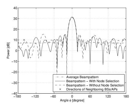
Figure 2: Beampattern: The intended BS/AP is located at $\varphi_{0}=0^{o}$ and $4$ neighboring BSs/APs at directions $\varphi_{1}=-160^{o}$, $\varphi_{2}=-50^{o}$, $\varphi_{2}=60^{o}$, and $\varphi_{3}=170^{o}$.

  In Fig. 2, we plot the sample beampattern corresponding to the CB with node selection and compare it to the sample beampattern corresponding to the CB without node selection and the average beampattern. The directions to the unintended BSs/APs are marked by symbol ‘$\times$’. It can be seen from the figure that the CB with node selection archives the lowest sidelobes in the directions of unintended BSs/APs, while the sidelobes of the CB without node selection are uncontrolled and high in the directions of unintended BSs/APs. Moreover, it can be seen that due to the CB coherent processing gain the peak of the mainlobe corresponds to 31 dB for all the beampatterns, while the power budget per all $N$ collaborative nodes was set to 20 dB. The latter can be also predicted by the theoretically computed gain increase of $\log_{10}N$ (see [3], [4]).

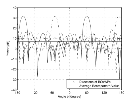
Figure 3: Beampattern: $4$ simultaneous beampatterns with BSs/APs at directions $\varphi_{1}=-160^{o}$, $\varphi_{2}=-50^{o}$, $\varphi_{2}=60^{o}$, and $\varphi_{3}=170^{o}$.

• In this case, it is required that the data from different sensor nodes have to be sent to all 4 BSs/APs simultaneously. Fig. 3 shows the CB beampatterns for the corresponding 4 CB clusters of 256 collaborative nodes selected from 512 nodes available in each cluster. Note that the sets of sensor nodes in all 4 CB clusters are different from each other and do not overlap.

  It can be seen from the figure that each beampattern has minimum interference at the direction of the mainlobes of the other beampatterns. Moreover, the mainlobes of the corresponding beampatterns all have the required mainlobes with a peak value of about 31 dB.

• In our third case, the neighboring BSs/APs are assumed to be located in the range $\phi\in[25^{o}\,45^{o}]$ which is closed to the mainlobe direction of the intended BS/AP. The INR threshold value is set to $\eta_{\text{thr}}=10$ dB.

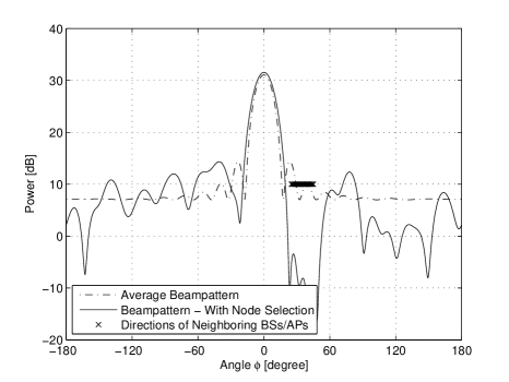
Figure 4: Beampattern: The neighboring BSs/APs are located in the range $\phi\in[25^{o}\,45^{o}]$ and $\eta_{\text{thr}}=10$ dB.

  The beampattern of the CB with node selection and the average beampattern are shown in Fig. 4. It can be seen from the figure that the CB with node selection is able to achieve a beampattern with sufficiently low sidelobes over the whole range $\phi\in[25^{o}\,45^{o}]$. Note that this case corresponds to the situation when the unintended AP is actually another cluster of sensor nodes distributed over space, which, therefore, cannot be viewed as a point in space.

• In the last case, we assume that $D=4$ neighboring untended Bs/APs are located at the angles corresponding to the peaks of the average beampattern, while the intended BS/AP is located at $\varphi_{0}=0^{o}$.

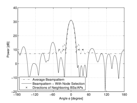
Figure 5: Beampattern: The neighboring BSs/APs are at directions corresponding to the peaks of the average beampattern.

  Fig. 5 shows the average beampattern and the beampattern of the CB with node selection. Note that the peaks of the average beampattern are located close to the mainlobe of the average beampattern. Therefore, the locations of the unintended BSs/APs are actually the worst locations in terms of the corresponding average interference levels. As it can be seen from the figure, using the node selection, we can achieve minimum interference levels at the directions of unintended BSs/APs even in this case.

Summarizing, it can be concluded based on all these cases that there is an significant improvement achieved by using the node selection algorithm in reducing the sidelobe levels at the directions of unintended BSs/APs.

V-B Effect of The Algorithm Parameters

The two parameters in the node selection algorithm are the INR threshold $\eta_{\text{thr}}$ and the size $L$ of the candidate set of nodes ${\cal L}^{k^{*}}\!\!$.

In this example, it is assumed that the intended BS/AP is located at $\varphi_{0}=0^{o}$ and there is one unintended neighboring BS/AP at the direction $\varphi_{1}=65^{o}$. The noise power equals to $\sigma_{w}^{2}=0.05$. The coverage area of the source node has a radius $R=5\lambda$. The INR threshold value changes in the range $\eta_{\text{thr}}=[-15\,10]$ dB. The parameters of the Gaussin distribution corresponding to the lognormal distribution of the channel coefficients are $m=0$ and $\sigma^{2}=0.2$. Monte Carlo simulations are carried over using $1000$ runs to obtain average results.

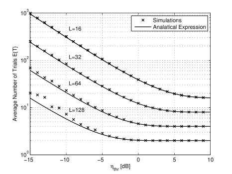
Figure 6: Average number of trials $E\left\{T\right\}$ versus threshold $\eta_{\text{thr}}$: $M=512$, $N=256$, $\varphi_{0}=0^{o}$, and $\varphi_{1}=65^{o}$.

Fig. 6 demonstrates the effect of the threshold $\eta_{\text{thr}}$ on the average number of trials required to select the set of collaborative nodes ${\cal N}^{k}$ using the sets of candidate nodes of different sizes $L\in\{16,32,64,128\}$. It can be seen from the figure that the curves obtained using the closed-form expression (21) for the number of trials are in good agreement with the simulation results. It can also be seen that by decreasing the threshold $\eta_{\text{thr}}$, the number of trials increases. Moreover, the number of trials can be controlled using $L$. Indeed, as $L$ increases, the number of trials decreases. It is important to note that because of the normalization factor in (11), the consumed power at each trial is the same for different values of $L$ and the total consumed power in the selection process is proportional to the number of trials.

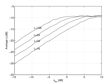
Figure 7: Average INR versus threshold $\eta_{\text{thr}}$: $M=512$, $N=256$, $\varphi_{0}=0^{o}$, and $\varphi_{1}=65^{o}$.

Fig. 7 shows the average interference level of the CB beampattern with node selection versus threshold $\eta_{\text{thr}}$ for different values of $L\in\{16,32,64,128\}$. It can be seen from the figure that the average interference level is proportional to the threshold $\eta_{\text{thr}}$. Comparing Figs. 6 and 7 to each other, we can observe a tradeoff between the average number of trials required for node selection and the achieved average interference (sidelobe) level. It can be seen that lower interference level can be achieved by using smaller values of $L$ at the expense of larger number of trials.

In addition, it is worth noting that there is no limitations in the node selection algorithm on selecting the value of $L$ as long as $L\leq N$. However, the threshold $\eta_{\text{thr}}$ affects the average interference level and, therefore, depends on the sensitivity of the front–end receiver of the BS/AP.

V-C Effect of Number of Neighboring BSs/APs

In this example, we study the effect of number of neighboring BSs/APs $D$ to the performance of the node selection algorithm. Note that for simplicity we have always assumed that $\eta_{\text{thr}}$ is the same for all BSs/APs. Such set up does not restrict the generality of the proposed node selection algorithm since the selection is performed based on the accept/regect bit from the corresponding BS/AP, while $\eta_{\text{thr}}$ is used only in the BS/AP. Therefore, it is straightforward to use different threshold values at different BSs/APs, and no changes to the node selection algorithm have to be done.

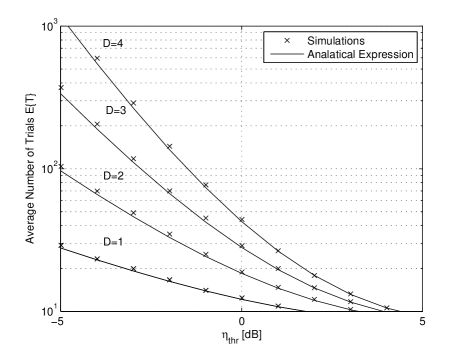
Figure 8: Average  number  of  trials  $E\left\{T\right\}$  versus  threshold  $\eta_{\text{thr}}$  for  different  values  of  $D$.

In Fig. 8, the average number of trials is plotted versus the threshold $\eta_{\text{thr}}$ for different values of $D\in\{1,2,3,4\}$. It can be seen from this figure that as $D$ increases, the average number of trials of the node selection algorithm increases exponentially if the required INR threshold $\eta_{\text{thr}}$ is low. Finally, it can be observed that the analytical and simulation results are in a good agreement with each other.

V-D The CCDF of the Beampattern Level

In our last example, we investigate the CCDF of the beampattern level.

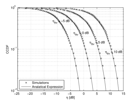
Figure 9: The CCDF of the INR for different values of the threshold $\eta_{\text{thr}}$: $M=512$, $N=256$, $L=32$, $\varphi_{0}=0^{o}$, and $\varphi_{1}=65^{o}$.

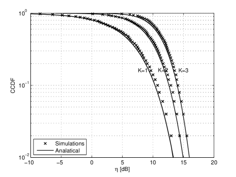
Figure 10: The CCDF of the INR for different values of $K$: $M=512$, $N=256$, $L=32$, $\varphi_{0}=0^{o}$, and $\eta_{\text{thr}}=10$ dB.

Fig. 9 depicts the probability that the interference exceeds certain level, i.e., it shows the CCDF of interference for different values of the INR threshold $\eta_{\text{thr}}\in\{-5,0,5,10\}$. In addition, Fig. 10 illustrates the CCDF of the interference for different numbers of active collaborative sets $K\in\{1,2,3\}$. It can be seen from Fig. 9 that the CCDF of the interference increases as $\eta_{\text{thr}}$ decreases. Moreover, as can be observed from Fig. 10, the CCDF of the interference increases if $K$ increases. The latter fact agrees with the intuition that for larger number of collaborative sets transmitting simultaneously, the overall received interference by all BSs/APs must be higher. The simulation results in both figures perfectly agree with our analytical results as well.

VI CONCLUSIONS

Node selection is introduced for the CB sidelobe control in the context WSNs. A low-overhead and efficient node selection algorithm is developed and analyzed. In particular, the expressions for the average number of trials required for the proposed node selection algorithm and the CCDF of the beampattern sidelobe level of the CB with node selection are derived. The effect of the number of nodes selected at one trial to the algorithm performance is also investigated. It is shown that increasing the number of nodes selected at one trial reduces the number of trials at the expense of higher sidelobe levels. It is also shown that the CCDF of the beampattern level depends on the interference threshold value. From both the analytical and simulation results, we have seen that CB with node selection has perfect interference suppression capabilities as compared to the CB without node selection for which the beampattern sidelobes are uncontrolled and can cause significant interference to unintended BSs/APs.

Appendix A: Derivation of the Mean and Variance of $x_{r}^{(k^{*},k)}$ and $y_{r}^{(k^{*},k)}$

First, we find the probability distribution of $u\in\left\{x_{r}^{(k^{*},k)},y_{r}^{(k^{*},k)}\right\}$ and then find the corresponding mean and variance. Assuming that the angles $\theta_{r}^{k}$ and $\theta_{r}^{k^{*}}$ are uniform distributed in the interval $[-\pi,\pi]$, i.e., $\theta\sim{\cal U}[-\pi,\pi]$, it can be found that the difference $\Delta=\theta_{r}^{k}-\theta_{r}^{k^{*}}$ has the following distribution

$$f(\Delta)=\left\{\begin{tabular}[]{ll}$\frac{2\pi-\Delta}{4\pi^{2}}$,&{$0\leq\Delta\leq 2\pi$;}\\ $\frac{2\pi+\Delta}{4\pi^{2}}$,&{$-2\pi\leq\Delta\leq 0$.}\end{tabular}\right.$$ (31)

Using the equality $u={\cal R}\left\{e^{j\Delta}\right\}=\cos\left(\Delta\right)$, we can find the roots of the equation $u=\cos\left(\Delta\right)$ in the interval $[-2\pi,2\pi]$ as

$$\Delta_{1} = \cos^{-1}(u)$$

$$\Delta_{2} = \pi+\cos^{-1}(u).$$ (32)

Then the distribution of $u$ can be found using the well known expression [28]

$$f(u)=\left.\frac{f(\Delta)}{|f^{\prime}(\Delta)|}\right|_{\Delta_{1},\Delta_{2}}$$ (33)

where $f^{\prime}(\Delta)$ is the first derivative of $f(\Delta)$.

Substituting (31) and (Appendix A: Derivation of the Mean and Variance of $x_{r}^{(k^{*},k)}$ and $y_{r}^{(k^{*},k)}$) into (33), and using the facts that $|u^{\prime}|=|-\sin(\Delta)|$ and $\sin(\cos^{-1}(u))=\sqrt{1-u^{2}}$, the distribution of $u$ can be found as

$$f(u)\!\! = \!\!\left.\frac{f(\Delta)}{\sin(\Delta)}\right|_{\Delta_{1},\Delta_{2}}$$ (34)

$$= \!\!\frac{2\pi-\cos^{-1}(u)}{2\pi^{2}\sin(\cos^{-1}(u))}+\frac{\pi-(\pi+\cos^{-1}(u))}{2\pi^{2}\sin(\pi+\cos^{-1}(u))}$$

$$= \!\!\frac{2\pi}{2\pi^{2}\sqrt{1-u^{2}}}=\frac{1}{\pi\sqrt{1-u^{2}}}.$$

The mean can be then easily found as

$$m_{u}=E\left\{u\right\}=\int_{-1}^{1}uf(u)du=\int_{-1}^{1}\frac{u}{\pi\sqrt{1-u^{2}}}du=\left.-\sqrt{1-u^{2}}\right|_{-1}^{1}=0.$$ (35)

And the variance can be found as

$$\sigma_{u}^{2}=E\left\{u^{2}\right\}=\int_{-1}^{1}u^{2}f(u)du=\int_{-1}^{1}\frac{u^{2}}{\pi\sqrt{1-u^{2}}}du=\left.\frac{\sin^{-1}(x)}{2\pi}\right|_{-1}^{1}-\left.\frac{u\sqrt{1-u^{2}}}{2\pi}\right|_{-1}^{1}=0.5.$$ (36)

Similar result can be also derived for $u\triangleq{\cal I}\left\{e^{j\Delta}\right\}=\sin\left(\Delta\right)$ in the same way.

Appendix B: Derivation of (21)

Consider an infinite sequence of independent Bernoulli trials with probability of success $p$. Let $Z_{1}$ denotes the number of trials before the first successful trial. Then $Z_{1}$ is geometric distributed random variable $Z_{1}\sim\text{Geom}(p)$, that is,

$${\bf Pr}(Z_{1}=k)=(1-p)^{k-1}p,\quad k=1,2,\cdots,\infty.$$ (37)

The corresponding moment generating function (MGF) for (37) is

$$M_{Z_{1}}(t)\!\! \triangleq \!\!E\{e^{tZ_{1}}\}=\sum_{k=1}^{\infty}e^{tk}(1-p)^{k-1}p$$ (38)

$$= \!\!pe^{t}\sum_{l=0}^{\infty}\left((1-p)e^{t}\right)^{l}=\frac{pe^{t}}{1-(1-p)e^{t}}.$$

Therefore, the average value of $Z_{1}$ can be found as

$$E\{Z_{1}\}\!\! = \!\!\left.\frac{d}{dt}M_{Z_{1}}(t)\right|_{t=0}=\left.\frac{(1-(1-p)e^{t})(pe^{t})-((p-1)e^{t})(pe^{t})}{(1-(1-p)e^{t})^{2}}\right|_{t=0}$$ (39)

$$= \!\!\left.\frac{pe^{t}}{(1-(1-p)e^{t})^{2}}\right|_{t=0}=\frac{p}{p^{2}}=\frac{1}{p}.$$

Similarly, we can find the average number of trials between the first and second successful trials $E\{Z_{2}\}$, second and third successful trials $E\{Z_{3}\}$, and so on until $T_{0}\triangleq N/L$ successful trial. Since $Z_{1},Z_{2},\cdots,Z_{T_{0}}$ are independent identically geometric distributed random variables, i.e., $Z_{i}\sim\text{Geom}(p)$, $\sum_{i=1}^{T_{0}}Z_{i}$ is negative geometric distributed, i.e., $\sum_{i=1}^{T_{0}}Z_{i}\sim\text{NegBin}(T_{0},p)$, with average

$$E\left\{\sum_{i=1}^{T_{0}}Z_{i}\right\}=T_{0}E\{Z_{i}\}=\frac{T_{0}}{p}=\frac{N}{L\cdot p}$$ (40)

where the fact that $Z_{1},Z_{2},\cdots,Z_{T_{0}}$ are independent identically distributed is used again.

References

- [1] D. Culler, D. Estrin, and M. Srivastava, “Overview of Sensor Networks,” Computer, vol. 37, no. 8, pp. 41–49, Aug. 2004.
- [2] I. F. Akyildiz, S. Weilian, Y. Sankarasubramaniam, and E. Cayirci, “A survey on sensor networks,” IEEE Communications Magazine, vol. 40, no. 8, pp. 102–114, Aug. 2002.
- [3] H. Ochiai, P. Mitran, H. V. Poor, and V. Tarokh, “Collaborative beamforming for distributed wireless ad hoc sensor networks,” IEEE Trans. on Signal Processing vol. 53, no. 11, pp. 4110–4124, Nov. 2005.
- [4] M. F. A. Ahmed and S. A. Vorobyov, “Collaborative beamforming for wireless sensor networks with Gaussian distributed sensor nodes,” IEEE Trans. on Wireless Communications, vol. 8, no. 2, pp. 638–643, Feb. 2009.
- [5] Z. Han and H. V. Poor, “Lifetime Improvement of Wireless Sensor Networks by Collaborative Beamforming and Cooperative Transmission,” in Proc. IEEE Internn Conf. Commun., Glasgow, Jun. 2007, pp. 3954–3958.
- [6] M. Kiese, C. Hartmann, J. Lamberty, R. Vilzmann, “On Connectivity Limits in Adhoc Networks with Beamforming Antennas,” Accepted in the EURASIP J. Wireless Commun. and Networking.
- [7] R. Mudumbai, B. Wild, U. Madhow, and K. Ramchandran, “Distributed Beamforming using 1 Bit Feedback: from Concept to Realization,” in Proc. Annual Allerton Conf. Commun. Control and Computing, Sep. 2006, pp. 1020-1027.
- [8] Q. Wang and K. Ren, “Time-Slotted Round-Trip Carrier Synchronization in Large-Scale Wireless Networks,” in Proc. IEEE Intern. Conf. Commun., Beijing, May 2008, pp. 5087–5091.
- [9] D. R. Brown and H. V. Poor, “Time-Slotted Round-Trip Carrier Synchronization for Distributed Beamforming,” IEEE Trans. on Signal Processing vol. 56, no. 11, pp. 5630–5643, Nov. 2008.
- [10] L. Dong, A. P. Petropulu, and H. V. Poor, “A Cross-Layer Approach to Collaborative Beamforming for Wireless Ad Hoc Networks,” IEEE Trans. on Signal Processing, vol. 56, pp. 2981–2993, Jul. 2008.
- [11] Y. Lo, “A mathematical theory of antenna arrays with randomly spaced elements,” IEEE Trans. Antennas and Propagation, vol. 12, no. 3, pp. 257–268, May 1964.
- [12] M. F. A. Ahmed and S. A. Vorobyov, “Performance characteristics of collaborative beamforming for wireless sensor networks with Gaussian distributed sensor nodes,” in Proc. IEEE Intern. Conf. Acoustics, Speech and Signal Processing, Las Vegas, NV, Mar.-Apr. 2008, pp. 3249–3252.
- [13] M. F. A. Ahmed and S. A. Vorobyov, “Beampattern random behavior in wireless sensor networks with Gaussian distributed sensor nodes,” in Proc. Canadian Conf. Electr. and Comp. Eng., May 2008, pp. 257–260.
- [14] R. Ramanathan, “On the performance of ad hoc networks with beamforming antennas,” ACM MobiHoc, 2001, pp. 95–105.
- [15] J. Liu and A. B. Gershman, Z. Q. Luo and K. M. Wong, “Adaptive beamforming with sidelobe control: a second-order cone programming approach,” IEEE Signal Processing Letters, vol. 10, no. 11, pp. 331–334, Nov. 2003.
- [16] K. L. Bell and H. L. Van Trees, “Adaptive and non-adaptive beampattern control using quadraticbeampattern constraints,” in Proc. 33rd Asilomar Conf. Signals, Systems, and Computers, Pacific Grove, CA, USA, 1999, pp. 486–490.
- [17] D. T. Hughes and J. G. McWhirter, “Sidelobe control in adaptive beamforming using a penalty function,” in Proc. ISSPA, Gold Coast, Australia, 1996.
- [18] M. F. A. Ahmed and S. A. Vorobyov, “Node selection for sidelobe control in collaborative beamforming for wireless sensor networks,” in Proc. IEEE 10th Workshop on Signal Processing Advances in Wireless Communications, Perugia, Jun 2009, pp. 519–523.
- [19] J. Yindi and H. Jafarkhani, “Network Beamforming with Channel Means and Covariances at Relays,” in Proc. IEEE Intern. Conf. Commun., Beijing, China, May 2008, pp. 3743–3747.
- [20] J. Yindi and H. Jafarkhani, “Network Beamforming using Relays with Perfect Channel Information,” in Proc. IEEE Intern. Conf. Acoustics, Speech and Signal Processing, Apr. 2007, pp. 473–476.
- [21] V. Havary-Nassab, S. Shahbazpanahi, A. Grami, and L. Zhi-Quan, “Distributed Beamforming for Relay Networks Based on Second-Order Statistics of the Channel State Information,” IEEE Transactions on Signal Processing, vol. 56, no. 9, pp. 4306–4316, Sep. 2008,
- [22] C. Lin, V. V. Veeravalli, and P. Meyn Sean, “Distributed Beamforming with Feedback: Convergence Analysis,” http://arxiv.org/abs/0806.3023, 2008-07-02.
- [23] A. P. Petropulu, L. Dong, and H. V.Poor, “Weighted Cross-Layer Cooperative Beamforming for Wireless Networks,” IEEE Trans. on Signal Processing, vol. 57, no. 8, pp. 3240–3252, Aug. 2009.
- [24] R. Lin and A. P. Petropulu, “A new wireless network medium access protocol based on cooperation,” IEEE Trans. on Signal Processing, vol. 53, no. 12, pp. 4675–4684, Dec. 2005.
- [25] Y. Hailong, A. P. Petropulu, Y. Xinhua, and T. Camp, “A Novel Location Relay Selection Scheme for ALLIANCES,” IEEE Trans. on Vehicular Technology, vol. 57, no. 2, pp. 1272–1284, Mar. 2008.
- [26] K. Zarifi, S. Affes, and A. Ghrayeb, “Distributed beamforming for wireless sensor networks with random node location,” in Proc. IEEE Intern. Conf. Acoustics, Speech and Signal Processing, Taipei, Taiwan, Apr. 2009, pp. 2261–2264.
- [27] Carl W. Helstrom, Probability and Stochastic Processes for Engineers, Macmillan Publishing Company, New York, 1984.
- [28] A. Papoulis, Probability, Random Variables, and Stochastic Processes Mc-Graw Hill, 1984.