Mixing times for random $\bolds k$-cycles and coalescence-fragmentation chains

Abstract

Let $\mathcal{S}_{n}$ be the permutation group on $n$ elements, and consider a random walk on $\mathcal{S}_{n}$ whose step distribution is uniform on $k$-cycles. We prove a well-known conjecture that the mixing time of this process is $(1/k)n\log n$, with threshold of width linear in $n$. Our proofs are elementary and purely probabilistic, and do not appeal to the representation theory of $\mathcal{S}_{n}$.

, and

t1Supported in part by EPSRC Grant EP/GO55068/1. t3Supported in part by NSF Grant DMS-08-04133 and by a grant from the Israel Science Foundation.

1 Introduction

1.1 Main result

Let $\mathcal{S}_{n}$ be the group of permutations of $\{1,\ldots,n\}$. Any permutation $\sigma\in\mathcal{S}_{n}$ has a unique cycle decomposition, which partitions the set $\{1,\ldots,n\}$ into orbits under the natural action of $\sigma$. The cycle structure of $\sigma$ is the integer partition of $n$ associated with this set partition, in other words, the ordered sizes of the cycles (blocks of the partition) ranked in decreasing size. It is customary not to include the fixed points of $\sigma$ in this structure. For instance, the permutation

$$\sigma=\pmatrix{1&2&3&4&5&6&7\cr 4&2&6&7&3&5&1}$$

has 3 cycles, $(1\enskip 4\enskip 7)(2)(3\enskip 6\enskip 5)$, so its cycle structure is $(3,3)$ (and one fixed point which does not appear in this structure). A conjugacy class $\Gamma\subset\mathcal{S}_{n}$ is the set of permutations having a given cycle structure. Let $|\Gamma|$ denote the support of $\Gamma$, that is, the number of nonfixed-points of any permutation $\sigma\in\Gamma$. In what follows we deal with the case where $\Gamma$ consists of a single $k$-cycle, in which case $|\Gamma|=k$ (see, however, Remark 2). It is well known and easy to see that in this case, if $k$ is even, then $\Gamma$ generates $\mathcal{S}_{n}$, while if $k>2$ is odd, then $\Gamma$ generates the alternate group $\mathcal{A}_{n}$ of even permutations. Let $(\pi_{t},t\geq 0)$ be the continuous-time random walk associated with $(\mathcal{S}_{n},\Gamma)$. That is, let $\gamma_{1},\gamma_{2},\ldots$ be a sequence of i.i.d. elements uniformly distributed on $\Gamma$, and let $(N_{t},t\geq 0)$ be an independent Poisson process with rate 1; then we take

$$\pi_{t}=\gamma_{1}\circ\cdots\circ\gamma_{N_{t}},$$ (1)

where $\gamma\circ\gamma^{\prime}$ indicates the composition of the permutations $\gamma$ and $\gamma^{\prime}$. $(\pi_{t},t\geq 0)$ is a Markov chain on $\mathcal{S}_{n}$ which converges to the uniform distribution $\mu$ on $\mathcal{S}_{n}$ when $|\Gamma|$ is even, and to the uniform distribution on $\mathcal{A}_{n}$ when $|\Gamma|>2$ is odd. In any case we shall write $\mu$ for that limiting distribution. We shall be interested in the mixing properties of this process as $n\to\infty$, as measured in terms of the total variation distance. Let $p_{t}(\cdot)$ be the distribution of $\pi_{t}$ on $\mathcal{S}_{n}$, and let $\mu$ be the invariant distribution of the chain. Let

$$d(t)=\|p_{t}(\cdot)-\mu\|=\frac{1}{2}\sum_{\sigma\in\mathcal{S}_{n}}|p_{t}(\sigma)-\mu(\sigma)|,$$

where $d(t)$ is the total variation distance between the state of the chain at time $t$ and its limiting distribution $\mu$. (Below, we will also use the notation $\|X-Y\|$ where $X$ and $Y$ are collections of random variables with laws $p_{X},p_{Y}$ to mean $\|p_{X}-p_{Y}\|$.)

The main goal of this paper is to prove that the chain exhibits a sharp cutoff, in the sense that $d(t)$ drops abruptly from its maximal value 1 to its minimal value 0 around a certain time $t_{\mathrm{mix}}$, called the mixing time of the chain. (See diaconis or LPW for a general introduction to mixing times.) Note that if $\Gamma$ is a fixed conjugacy class of $\mathcal{S}_{n}$ and $m>n$, $\Gamma$ can also be considered a conjugacy class of $\mathcal{S}_{m}$ by simply adding $m-n$ fixed points to any permutation $\sigma\in\Gamma$. With this in mind, our theorem states the following:

Theorem 1

Let $k\geq 2$ be an integer, and let $\Gamma_{k}$ be the conjugacy class of $\mathcal{S}_{n}$ corresponding to $k$-cycles. The continuous time random walk $(\pi_{t},t\geq 0)$ associated with $(\mathcal{S}_{n},\Gamma_{k})$ has a cutoff at time $t_{\mathrm{mix}}:=(1/k)n\log n$, in the sense that for any $\varepsilon>0$, there exist $N_{\varepsilon,k},C_{\varepsilon,k}>0$ large enough so that for all $n\geq N_{\varepsilon,k}$,

$$d(t_{\mathrm{mix}}-C_{\varepsilon,k}n) > 1-\varepsilon,$$ (2)

$$d(t_{\mathrm{mix}}+C_{\varepsilon,k}n) < \varepsilon.$$ (3)

As explained in Section 1.2 below, this result solves a well-known conjecture formulated by several people over the course of the years.

Remark 2.

Theorem 1 can be extended, without a significant change in the proofs, to cover the case of general fixed conjugacy classes $\Gamma$, with $k=|\Gamma|>2$ independent of $n$. In order to alleviate notation, we present here only the proof for $k$-cycles. A more delicate question, that we do not investigate, is what growth of $k=k(n)$ is allowed so that Theorem 1 would still be true in the form

$$d\bigl{(}t_{\mathrm{mix}}(1-\delta)\bigr{)} > 1-\varepsilon,$$ (4)

$$d\bigl{(}t_{\mathrm{mix}}(1+\delta)\bigr{)} < \varepsilon?$$ (5)

The lower bound in (4) is easy. For the upper bound in (5), due to the birthday problem, the case $k=o(\sqrt{n})$ should be fairly similar to the arguments we develop below, with adaptations in several places, for example, in the argument following (32); we have not checked the details. Things are likely to become more delicate when $k$ is of order $\sqrt{n}$ or larger. Yet, we conjecture that (5) holds as long as $k=o(n)$.

1.2 Background

This problem has a rather long history, which we now sketch. Mixing times of Markov chains were studied independently by Aldous aldous-mix and by Diaconis and Shahshahani d-sh at around the same time, in the early 1980s. Diaconis and Shahshahani d-sh , in particular, establish the existence of what has become known as the cutoff phenomenon for the composition of random transpositions. Random transpositions is perhaps the simplest example of a random walk on $\mathcal{S}_{n}$ and is a particular case of the walks covered in this paper, arising when the conjugacy class $\Gamma$ contains exactly all transpositions. The authors of d-sh obtained a version of Theorem 1 for this particular case (with explicit choices of $C_{2,\varepsilon}$ for a given $\varepsilon$). As is the case here, the hard part of the result is the upper-bound (3). Remarkably, their solution involved a connection with the representation theory of $\mathcal{S}_{n}$, and uses rather delicate estimates on so-called character ratios.

Soon afterwards, a flurry of papers tried to generalize the results of d-sh in the direction we are taking in this paper, that is, when the step distribution is uniform over a fixed conjugacy class $\Gamma$. However, the estimates on character ratios that are needed become harder and harder as $|\Gamma|$ increases. Flatto, Odlyzko and Wales FOW , building on earlier work of Vershik and Kerov vk , obtained finer estimates on character ratios and were able to show that mixing must occur before $(1/2)n\log n$ for $|\Gamma|$ fixed, thus giving another proof of the Diaconis–Shahshahani result when $|\Gamma|=2$. (Although this does not appear explicitly in FOW , it is recounted in Diaconis’s book diaconis , page 44.) Improving further the estimates on character ratios, Roichman roichman1 , roichman2 was able to prove a weak version of Theorem 1, where it is shown that $d(t)$ is small if $t>Ct_{\mathrm{mix}}$ for some large enough $C>0$. In his result, $|\Gamma|$ is allowed to grow to infinity as fast as $(1-\delta)n$ for any $\delta>0$. To our knowledge, it is in roichman1 that Theorem 1 first formally appears as a conjecture, although we have no doubt that it had been privately made before. (The lower bound for random transpositions, which is based on counting the number of fixed points in $\pi_{t}$, works equally well in this context and provides the conjectured correct answer in all cases.) Lulov lulov dedicated his Ph.D. thesis to the problem, and Lulov and Pak lulov-pak obtained a partial proof of the conjecture of Roichman, in the case where $|\Gamma|$ is very large, that is, greater than $n/2$. More recently, Roussel roussel1 and roussel2 made some progress in the small $|\Gamma|$ case, working out the character ratios estimates to treat the case where $|\Gamma|\leq 6$. Saloff-Coste, in his survey article (lsc , Section 9.3) discusses the sort of difficulties that arise in these computations and states the conjecture again. A summary of the results discussed above is also given. See also SZ , page 381, where work in progress of Schlage-Puchta that overlaps the result in Theorem 1 is mentioned.

1.3 Structure of the proof

To prove Theorem 1, it suffices to look at the cycle structure of $\pi_{t}$ and check that if $N_{t}(i)$ is the number of cycles of $\pi_{t}$ of size $i$ for every $i\geq 1$, and if $t\geq t_{\mathrm{mix}}+C_{k,\varepsilon}n$ then the total variation distance between $(N_{t}(i))_{1\leq i\leq n}$ and $(N(i))_{1\leq i\leq n}$ is close to 0, where $(N(i))_{1\leq i\leq n}$ is the cycle distribution of a random permutation sampled from $\mu$. We thus study the dynamics of the cycle distribution of $\pi_{t}$, which we view as a certain coagulation–fragmentation chain. Using ideas from Schramm schramm , it can be shown that large cycles are at equilibrium much before $t_{\mathrm{mix}}$, that is, at a time of order $O(n)$. Very informally speaking, the idea of the proof is the following. We focus for a moment on the case $k=2$ of random transpositions, which is the easiest to explain. The process $(\pi_{t},t\geq 0)$ may be compared to an Erdős–Rényi random graph process $(G_{t},t\geq 0)$ where random edges are added to the graph at rate 1, in such a way that the cycles of the permutation are subsets of the connected components of $G_{t}$. Schramm’s result from schramm then says that, if $t=cn$ with $c>1/2$ (so that $G_{t}$ has a giant component), then the macroscopic cycles within the giant component have relaxed to equilibrium. By an old result of Erdős and Rényi, it takes time $t=t_{\mathrm{mix}}+C_{k,\varepsilon}n$ for $G_{t}$ to be connected with probability greater than $1-\varepsilon$. By this point the giant component encompasses every vertex and thus, extrapolating Schramm’s result to this time, the macroscopic cycles of $\pi_{t}$ have the correct distribution at this point. A separate and somewhat more technical argument is needed to deal with small cycles.

More formally, the proof of Theorem 1 thus proceeds in two main steps. In the first step, presented in Section 2 and culminating in Proposition 18, we show that after time $t_{\mathrm{mix}}+c_{\varepsilon,k}n$, the distribution of small cycles is close (in variation distance) to the invariant measure, where a small cycle means that it is smaller than a suitably chosen threshold approximately equal to $n^{7/8}$. This is achieved by combining a queueing-system argument (whereby initial discrepancies are cleared by time slightly larger than $t_{\mathrm{mix}}$ and equilibrium is achieved) with a priori rough estimates on the decay of mass in small cycles (Section 2.1). In the second step, contained in Section 3, a variant of Schramm’s coupling from schramm is presented, which allows us to couple the chain after time $t_{\mathrm{mix}}+c_{\varepsilon,k}n$ to a chain started from equilibrium, within time of order $n^{5/8}\log n$, if all small cycles agree initially.

2 Small cycles

In this section we prove the following proposition. Let $(N_{i}(t))_{1\leq i\leq n}$ be the number of cycles of size $i$ of the permutation $\pi_{t}$, where $(\pi_{t},t\geq 0)$ evolves according to random $k$-cycles (where $k\geq 2$), but does not necessarily start at the identity permutation. Let $(Z_{i})_{i=1}^{n}$ denote independent Poisson random variables with mean $1/i$.

Fix $0<\chi<1$ and let $K=K(n)$ be the closest dyadic integer to $n^{\chi}$. We think of cycles smaller than $K$ as being small, and big otherwise. Let $I_{j}=\{i\in\mathbb{Z}\dvtx i\in[2^{j},2^{j+1})\}$, $L_{j}=|I_{j}|=2^{j}$ and

$$M_{j}(t)=\sum_{i\in I_{j}}N_{i}(t).$$ (6)

Introduce the stopping time

$$\tau=\inf\{t\geq 0\dvtx\exists 0\leq j\leq\log_{2}K+1,M_{j}(t)>(\log n)^{6}/2\}.$$ (7)

Therefore, prior to $\tau$, the total number of small cycles in each dyadic strip $[2^{j}$, $2^{j+1})$ $(j\leq 1+\log_{2}K)$ never exceeds $(\log n)^{6}/2$.

Proposition 3

Suppose that

$$\mathbb{P}(\tau<n\log n)\longrightarrow 0$$ (8)

as $n\to\infty$, and that initially,

$$M_{j}(0)\leq D\log(j+2)$$ (9)

for all $0\leq j\leq\log_{2}\log n$, for some $D>0$ independent of $j$ or $n$. Then for any sequence $t=t(n)$ such that $t(n)/n\to\infty$ as $n\to\infty$ and $t(n)\leq n\log n$,

$$\|(N_{i}(t))_{i=1}^{K}-(Z_{i})_{i=1}^{K}\|\longrightarrow 0.$$

In particular, under the assumptions of Proposition 3, for any $\varepsilon>0$ there is a $c_{\varepsilon,k}>0$ such that for all $n$ large,

$$\|(N_{i}(c_{\varepsilon,k}n))_{i=1}^{K}-(Z_{i})_{i=1}^{K}\|<\varepsilon.$$

In Sections 2.1 and 2.4, Proposition 3 is applied to the chain after time roughly $t_{\mathrm{mix}}=(n\log n)/k$, at which point the initial conditions $M_{j}(0)$ satisfy (9) (with high probability). Proof of Proposition 3 The proof of this proposition relies on the analysis of the dynamics of the small cycles, where each step of the dynamics corresponds to an application of a $k$-cycle, by viewing it as a coagulation–fragmentation process. To start with, note that every $k$-cycle may decomposed as a product of $k-1$ transpositions

$$c=(x_{k},\ldots,x_{1})=(x_{k},x_{k-1})\cdots(x_{2},x_{1}).$$

Thus the application of a $k$-cycle may be decomposed into the application of $k-1$ transpositions: namely, applying $c$ is the same as first applying the transposition $(x_{1},x_{2})$ followed by $(x_{2},x_{3})$ and so on until $(x_{k-1},x_{k})$. Whenever one of those transpositions is applied, say $(a,b)$, this can yield either a fragmentation or a coagulation, depending on whether $a$ and $b$ are in the same cycle or not at this time. If they are, say if $b=\sigma^{i}(a)$ (where $i\geq 1$ and $\sigma$ denotes the permutation at this time), then the cycle $C$ containing $a$ and $b$ splits into $(a,\ldots,\sigma^{i-1}(a))$ and everything else, that is, $(b,\ldots,\sigma^{|C|-i}(b))$. If they are in different cycles $C$ and $C^{\prime}$ then the two cycles merge.

To track the evolution of cycles, we color the cycles with different colors (blue, red or black) according (roughly) to the following rules. The blue cycles will be the large ones, and the small ones consist of red and black. Essentially, red cycles are those which undergo a “normal” evolution, while the black ones are those which have experienced some kind of error. By “normal evolution,” we mean the following: in a given step, one small cycle is generated by fragmentation of a blue cycle. It is the first small cycle that is involved in this step. In a later step of the random walk, this cycle coagulates with a large cycle and thus becomes large again. If at any point of this story, something unexpected happens (e.g., this cycle gets fragmented instead of coagulating with a large cycle, or coagulates with another small cycle) we will color it black. In addition, we introduce ghost cycles to compensate for this sort of error.

We now describe this procedure more precisely. We start by coloring every cycle of the permutation $\sigma(t)$ which is larger than $K$ blue. We denote by $\theta(t)$ the fraction of mass contained in blue cycles, that is,

$$\theta(t)=\frac{1}{n}\sum_{i=K+1}^{n}iN_{i}(t).$$ (10)

Note that by definition of $\tau$,

$$1-\frac{K}{n}(\log n)^{6}\leq\theta(t)\leq 1$$ (11)

for all $t\leq\tau$.

We now color the cycles which are smaller than $K$ either red or black according to the following dynamics. Suppose we are applying a certain $k$-cycle $c=(x_{k},\ldots,x_{1})$, which we write as a product of $k-1$ transpositions

$$c=(x_{k},\ldots,x_{1})=(x_{k},x_{k-1})\cdots(x_{2},x_{1})$$ (12)

(note that we require that $x_{i}\neq x_{j}$ for $i\neq j$).

Red cycles. Assume that a blue cycle is fragmented and one of the pieces is small, and that this transposition is the first one in the application of the $k$-cycle $(x_{1},\ldots,x_{k})$ to involve a small cycle. In that case (and only in that case), we color it red. Red cycles may depart through coagulation or fragmentation. A coagulation with a blue cycle, if it is the first in the step and no small cycles were created in this step prior to it, will be called lawful. Any other departure will be called unlawful. If a blue cycle breaks up in a way that would create a red cycle and both cycles created are small (which may happen if the size of the cycle is between $K$ and $2K$), then we color the smaller one red and the larger one black, with a random rule in the case of ties.

Black cycles. Black cycles are created in one of two ways. First, any red cycle that departs in an unlawful fashion and stays small becomes black. Further, if the transposition $(a,b)$ is not the first transposition in this step to create a small cycle from a blue cycle, or if it is but a previous transposition in the step involved a small cycle, then the small cycle(s) created is colored black. Now, assume that $(a,b)$ involves only cycles which are smaller than $K$: this may be a fragmentation producing two new cycles, or a merging of two cycles producing one new cycle. In this case, we color the new cycle(s) black, no matter what the initial color of the cycles, except if this operation is a coagulation and the size of this new cycle exceeds $K$, in which case it is colored blue again. Thus, black cycles are created through either coagulations of small parts or fragmentation of either small or large parts, but black cycles disappear only through coagulation.

We aim to analyze the dynamics of the red and black system, and the idea is that the dynamics of this system are essentially dominated by that of the red cycles, where the occurrence of black cycles is an error that we aim to control.

Ghosts. Let $R_{i}(t),B_{i}(t)$ be the number of red and black cycles, respectively, of size $i$ at time $t$. It will be helpful to introduce another type of cycle, called ghost cycles, which are nonexisting cycles which we add for counting purposes: the point is that we do not want to touch more than one red cycle in any given step. Thus, for any red cycle departing in an unlawful way, we compensate it by creating a ghost cycle of the same size. For instance, suppose two red cycles $C_{1}$ and $C_{2}$ coagulate (this could form a blue or a black cycle). Then we leave in the place of $C_{1}$ and $C_{2}$ two ghost cycles $C^{\prime}_{1}$ and $C^{\prime}_{2}$ of sizes identical to $C_{1}$ and $C_{2}$.

An exception to this rule is that if, during a step, a transposition creates a small red cycle by fragmentation of a blue cycle, and later within the same step this red cycle either is immediately fragmented again in the next transposition or coagulates with another red or black cycle and remains small, then it becomes black as above but we do not leave a ghost in its place.

Finally, we also declare that every ghost cycle of size $i$ is killed independently of anything else at an instantaneous rate which is precisely given by $i\mu(t)$, where $\mu(t)$ is a random nonnegative number (depending on the state of the system at time $t$) which will be defined below in (17) and corresponds to the rate of lawful departures of red cycles.

To summarize, we begin at time $0$ with all large cycles colored blue and all small cycles colored red. For every step consisting of $k$ transpositions, we run the following algorithm for the coloring of small cycles and creation of ghost cycles (see Table 1).

Table 1: Coloring algorithm for small cycles, and creation of ghost cycles

• If the transposition is a fragmentation, go to (F); otherwise, go to (C).

• If the fragmentation is of a small cycle $c$ of length $\ell$, go to (FS); otherwise, go to (FL).

• Color the resulting small cycles black. Create a ghost cycle of length $\ell$, except if $c$ was created in the previous transposition of the current step and is red. Finish.

• If the fragmentation creates one or two small cycles, and this transposition is the first in the step to either create or involve a small cycle, color the smallest small cycle created red. All other small cycles created are colored black. Do not create ghost cycles. Finish.

• If the coagulation involves a blue cycle, go to (CL); otherwise, go to (CS).

• If the blue cycle coagulates with a red cycle, and this is not the first transposition in the step that involves a small cycle, then create a ghost cycle; otherwise, do not create a ghost cycle. Finish.

• If a small cycle remains after the coagulation, it is colored black. If the coagulation involved two red cycles of size $\ell$ and $\ell^{\prime}$, create two ghost cycles of sizes $\ell$ and $\ell^{\prime}$, unless one of these two red cycles (say of size $\ell^{\prime}$) was created in the current step, in which case create only one ghost cycle of size $\ell$. Finish.

[]In addition to this description, all ghost cycles are killed instantaneously at rate $\mu(t)$ defined in (17).

Let $G_{i}(t)$ denote the number of ghost cycles of size $i$ at time $t$, and let $Y_{i}=R_{i}+G_{i}$, which counts the number of red and ghost cycles of size $i$. Our goal is twofold. First, we want to show that $(Y_{i}(t))_{i=1}^{K}$ is close in total variation distance to $(Z_{i})_{i=1}^{K}$ and second, that at time $t=t(n)$ the probability that there is any black cycle or a ghost cycle converges to 0 as $n\to\infty$.

Remark 4.

Note that with our definitions, at each step at most one red cycle can be created, and at most one red cycle can disappear without being compensated by the creation of a ghost. Furthermore these two events cannot occur in the same step.

Lemma 5

Assume (8) as well as (9), and let $t=t(n)$ be as in Proposition 3. Then

$$\|(Y_{i}(t))_{i=1}^{K}-(Z_{i})_{i=1}^{K}\|\longrightarrow 0.$$

The idea is to observe that $Y_{i}$ has approximately the following dynamics:

$$\cases{\mbox{rate: }(x\to x+1)=\lambda,&\quad if $x\geq 0$,\cr\mbox{rate: }(x\to x-1)=ix\mu,&\quad if $x\geq 1$,}$$

and that $\lambda=\mu=k/n+o(1/n)$, so that $(Y_{i})$ is approximately a system of $M/M/\infty$ queues where the arrival rate is $k/n$ and the departure rate of every customer is $ik/n$. The equilibrium distribution of $(Y_{i})$ is thus approximately Poisson with parameter the ratio of the two rates, that is, $1/i$. The number of initial customers in the queues is, by assumption (8), small enough so that by time $t(n)$ they are all gone, and thus the queue has reached equilibrium.

We now make this heuristics precise. To increase $Y_{i}$ by 1, that is, to create a red cycle, one needs to specify the $j$th transposition, $1\leq j\leq k-1$, of the $k$-cycle at which it is created. The first point $x_{1}$ of the $k$-cycle must fall somewhere in a blue cycle (which has probability $\theta$). Say that $x_{1}\in C_{1}$, with $C_{1}$ a blue cycle. In order to create a cycle of size exactly $i$ at this transposition, the second point $x_{2}$ must fall at either of exactly two places within $C_{1}$: either $\sigma^{i}(x_{1})$ or $\sigma^{-i}(x_{1})$. However, note that if $x_{2}=\sigma^{-i}(x_{1})$ and $|c|=k\geq 3$, then the next transposition is guaranteed to involve the newly formed cycle, either to reabsorb it in the blue cycles, or to turn into a black cycle through coalescence with another small cycle or fragmentation. Either way, this newly formed cycle does not eventually lead to an increase in $Y_{i}$ since by our conventions, we do not leave a ghost in its place. On the other hand, if $x_{2}=\sigma^{i}(x_{1})$ then the newly formed red cycle will stay on as a red or a ghost cycle in the next transpositions of the application of the cycle $c$. Whether it stays as a ghost or a red cycle does not change the value of $Y_{i}$, and therefore, this event leads to a net increase of $Y_{i}$ by 1. This is true for all of the first $k-2$ transpositions of the $k$-cycle $c$, but not for the last one, where both $x_{k}=\sigma^{i}(x_{k-1})$ and $x_{k}=\sigma^{-i}(x_{k-1})$ will create a red cycle of size $i$. It follows from this analysis that the total rate $\lambda(t)$ at which $Y_{i}$ increases by 1 satisfies

$$\lambda(t)\leq\lambda^{+}=\frac{k-2}{n-k+1}+\frac{2}{n-k+1}=\frac{k}{n-k+1}.$$ (13)

To get a lower bound, observe that for $t\leq\tau$, $\theta(t)\geq 1-K(\log n)^{6}/n$ at the beginning of the step. When a $k$-cycle is applied and we decompose it into $k-1$ elementary transpositions, the value $\theta(t)$ for each of the transpositions may take different successive values which we denote by $\theta(t,j),j=1,\ldots,k-1$. However, note that at each such transposition, $\theta$ can only change by at most $\pm 2K/n$. Thus it is also the case that for all $1\leq j\leq k-1$, $\theta(t,j)\geq 1-2(k-1)K(\log n)^{6}/n$. Therefore, the probability that a fragmentation of a blue cycle does not create any small cycle is also bounded below by

$$1-2(k-1)K(\log n)^{6}/n-2K(\log n)^{6}/n=1-2kK(\log n)^{6}/n=:\theta_{-}(t).$$

It thus follows that the total rate $\lambda(t)$ is bounded below by

$$\lambda(t)\geq\theta_{-}^{k-1}\biggl{(}\frac{2}{n}+\frac{k-2}{n}\biggr{)}\geq\frac{k}{n}\biggl{(}1-8k\frac{K(\log n)^{6}}{n}\biggr{)}=:\lambda^{-}.$$ (14)

Of course, by this we mean that the $Y_{i}(t)$ are nonnegative jump processes whose jumps are of size $\pm 1$, and that if $\mathcal{F}_{t}$ is the filtration generated by the entire process up to time $t$, then

$$\qquad\lim_{h\to 0^{+}}\frac{\mathbb{P}(Y_{i}(t+h)=x+1|\mathcal{F}_{t},Y_{i}(t)=x)}{h}=\lambda(t)\quad\mbox{and}\quad\lambda^{-}\leq\lambda(t)\leq\lambda^{+}$$ (15)

almost surely on the event $\{t\leq\tau\}$. As for negative jumps, we have that for $x\geq 1$,

$$\lim_{h\to 0^{+}}\frac{\mathbb{P}(Y_{i}(t+h)=x-1|\mathcal{F}_{t},Y_{i}(t)=x)}{h}=ix\mu(t),$$ (16)

where $\mu(t)$ depends on the partition and satisfies the estimates

$$\mu^{-}\leq\mu(t)\leq\mu^{+},$$ (17)

where

$$\mu^{-}:=\frac{k}{n}\biggl{(}1-8k\frac{K(\log n)^{6}}{n}\biggr{)}\quad\mbox{and}\quad\mu^{+}=\frac{k}{n-k}.$$ (18)

The reason for this is as follows. To decrease $Y_{i}$ by 1 by decreasing $R_{i}$, note that the only way to get rid of a red cycle without creating a ghost is to coagulate it with a blue cycle at the $j$th transposition, $1\leq j\leq k-1$, with no other transpositions creating small cycles. The probability of this event is bounded above by $ik/(n-k)$ and, with $\theta_{-}$ as above, bounded below by

$$\frac{i\theta}{n}\theta_{-}^{k-2}+\theta\frac{i}{n-1}\theta_{-}^{k-2}+\theta\theta_{-}\frac{i}{n-2}\theta_{-}^{k-3}+\cdots+\theta\theta_{-}^{k-2}\frac{i}{n-k+1}\geq\frac{ik}{n}\theta_{-}^{k-1}.$$

Therefore, if in addition ghosts are each killed independently with rate $\mu(t)$ as above, then (16) holds. More generally, if $1\leq m\leq K$ and $i_{1}<\cdots<i_{m}\leq K$ are pairwise distinct integers, then we may consider the vector $(Y_{i_{1}}(t),\ldots,Y_{i_{m}}(t))$. If its current state is $x=(x_{1},\ldots,x_{m})$, then it may make transitions to $x^{\prime}=(x^{\prime}_{1},\ldots,x^{\prime}_{m})$ where the two vectors $x$ and $x^{\prime}$ differ by exactly one coordinate (say the $j$th one) and $x_{j}-x^{\prime}_{j}=\pm 1$ (since only one queue $Y_{i}$ can change at any time step, thanks to our coloring rules). Also, writing $Y(t)$ for the vector $(Y_{i_{1}}(t),\ldots,Y_{i_{m}}(t))$, we find

$$\lim_{h\to 0^{+}}\frac{\mathbb{P}(Y(t+h)=x^{\prime}|\mathcal{F}_{t},Y=x)}{h}=\cases{\lambda(t),&\quad if $x^{\prime}_{j}=x_{j}+1$,\cr i_{j}x_{j}\mu(t),&\quad if $x^{\prime}_{j}=x_{j}-1$.}$$

These observations show that we can compare $\{(Y_{i}(t\wedge\tau)_{1\leq i\leq K},t\geq 0\}$ to a system of independent Markov queues $\{(Y^{+}_{i}(t\wedge\tau))_{1\leq i\leq K},t\geq 0\}$ with respect to a common filtration $\mathcal{F}_{t}$, with no simultaneous jumps almost surely, and such that the arrival rate of each $Y_{i}$ is $\lambda^{+}$, and the departure rate of each client in $Y_{i}$ is $i\mu^{-}$. We may also define a system of queues $(Y^{-}_{i})_{1\leq i\leq K}$ by accepting every new client of $Y^{+}_{i}$ with probability $\lambda^{-}/\lambda^{+}$ and rejecting it otherwise. Subsequently, each accepted client tries to depart at a rate $\mu^{+}-\mu^{-}$, or when it departs in $Y^{+}_{i}$, whichever comes first. Then one can construct all three processes $(Y^{-}_{i})_{1\leq i\leq K}$, $(Y_{i})_{1\leq i\leq K}$ and $(Y^{+}_{i})_{1\leq i\leq K}$ on a common probability space in such a way that $Y^{-}_{i}(t)\leq Y_{i}(t)\leq Y^{+}_{i}(t)$ for all $t\leq\tau$.

Note that if $(Z^{+}_{i})_{1\leq i\leq K}$ denote independent Poisson random variables with mean $\lambda^{+}/(i\mu^{-})$, then $(Z^{+}_{i})_{1\leq i\leq K}$ forms an invariant distribution for the system $(Y^{+}_{i}(t),t\geq 0)_{1\leq i\leq K}$. Let $(Z^{+}_{i}(t),t\geq 0)_{1\leq i\leq K}$ denote the system of Markov queues $Y^{+}_{i}$ started from its equilibrium distribution $(Z^{+}_{i})_{1\leq i\leq K}$. Then $(Y^{+}_{i}(t))_{1\leq i\leq K}$ and $(Z^{+}_{i}(t))_{1\leq i\leq K}$ can be coupled as usual by taking each coordinate to be equal after the first time that they coincide. In particular, once all the initial customers of $Y^{+}_{i}$ and of $Z^{+}_{i}(t)$ have departed (let us call $\tau^{\prime}$ this time), then the two processes $(Y^{+}_{i})_{1\leq i\leq K}$ and $(Z^{+}_{i})_{1\leq i\leq K}$ are identical.

We now check that this happens before $t=t(n)$ with high probability. It is an easy exercise to check this for $Z^{+}_{i}(t)$ so we focus on $Y^{+}_{i}(t)$. To see this, note that by (9), there are no more than $D\log(j+2)$ customers in every strip $[2^{j},2^{j+1})$ initially if $j\leq\log_{2}\log n$. Moreover, each customer departs with rate at least $2^{j-1}/n$ when in this strip. Thus the time $\tau^{\prime}_{j}$ it takes for all initial customers of $Y^{+}$ in strip $[2^{j},2^{j+1})$ to depart is dominated by $(n/2^{j-1})\max_{1\leq q\leq D\log(j+2)}E_{q}$, where $(E_{q})_{q\geq 1}$ is a collection of i.i.d. standard exponential random variables. Hence

$$\mathbb{E}(\tau^{\prime}_{j})\leq\frac{n}{2^{j-2}}\bigl{(}\log_{2}D+\log\log(j+4)\bigr{)}.$$

For larger strips we use the crude and obvious bound $M_{j}(0)\leq n$ if $j\geq\log_{2}\log n$. Moreover, each customer departs at rate $2^{j-1}/n$ with $j\geq\break\lfloor\log_{2}\log n\rfloor$. Thus, in distribution,

$$\tau^{\prime}_{j}\preceq\frac{n}{2^{j-2}}\max_{1\leq q\leq n}E_{q}$$

so that $\mathbb{E}(\tau^{\prime}_{j})\leq n\log n/2^{j-1}$ [we are using here that $\mathbb{E}(\max_{1\leq q\leq m}E_{q})\leq 2\log m$ for all $m$ large enough]. Since we obviously have $\tau^{\prime}\leq\sum_{j=0}^{\log_{2}K+1}\tau^{\prime}_{j}$, we conclude

$$\mathbb{E}(\tau^{\prime})\leq\sum_{j=0}^{\log_{2}\log n}\frac{n}{2^{j-2}}\bigl{(}\log D+\log\log(j+4)\bigr{)}+\sum_{j\geq\log_{2}\log n}\frac{n\log n}{2^{j-1}}\leq a(D)n,$$

where $a(D)<\infty$ depends solely on $D$. By Markov’s inequality and since $t(n)/n\to\infty$, we conclude that $\tau^{\prime}\leq t$ with high probability. We now claim that $(Y_{i}^{-}(t))_{1\leq i\leq K}=(Y_{i}^{+}(t))_{1\leq i\leq K}$ with high probability. To see this, we note that at equilibrium $\mathbb{E}(Z^{+}_{i})=\lambda^{+}/(i\mu^{-})\leq 2/i$. Therefore,

$$\mathbb{P}\bigl{(}Y^{+}_{i}(t)\neq Y^{-}_{i}(t)\mbox{ for some $1\leq i\leq K$}\bigr{)}$$

$$\qquad\leq\mathbb{E}\Biggl{(}\sum_{i=1}^{K}Y^{+}_{i}(t)-Y^{-}_{i}(t);\tau^{\prime}<t\Biggr{)}+\mathbb{P}(\tau^{\prime}>t)$$

$$\qquad\leq\sum_{i=1}^{K}\frac{2}{i}\biggl{\{}\biggl{(}1-\frac{\lambda^{-}}{\lambda^{+}}\biggr{)}+\biggl{(}1-\frac{\mu^{-}}{\mu^{+}}\biggr{)}\biggr{\}}+\mathbb{P}(\tau^{\prime}>t)$$

$$\qquad\leq 16(k-1)\frac{K(\log n)^{7}}{n}+\mathbb{P}(\tau^{\prime}>t).$$

Since we have already checked that $\mathbb{P}(\tau^{\prime}>t)\to 0$ as $n\to\infty$, this shows that on the event $\{\tau^{\prime}\leq t\leq\tau\}$ and $\{Y^{+}_{i}(t)=Y^{-}_{i}(t)\mbox{ for all }1\leq i\leq K\}$ (an event of probability asymptotically one), $(Y_{i}(t))_{1\leq i\leq K}$ can be coupled to $(Z^{+}_{i}(t))_{1\leq i\leq K}$ which has the same law as $(Z^{+}_{i})_{1\leq i\leq K}$. Thus

$$\|(Y_{i})_{i=1}^{K}-(Z^{+}_{i})_{i=1}^{K}\|\longrightarrow 0$$ (19)

as $n\to\infty$. On the other hand, we claim that

$$\|(Z_{i})_{i=1}^{K}-(Z^{+}_{i})_{i=1}^{K}\|\longrightarrow 0$$

also. Indeed, it is easy to see and well known that for $\alpha,\beta>0$

$$\|\mathrm{Po}(\alpha)-\operatorname{Po}(\beta)\|\leq 1-\exp(-|\alpha-\beta|)\leq|\alpha-\beta|.$$

Since the coordinates of $Z_{i}$ and $Z^{+}_{i}$ are both independent Poisson random variables but with different parameters, we find that

$$\|(Z_{i})_{i=1}^{K}-(Z^{+}_{i})_{i=1}^{K}\| \leq \sum_{i=1}^{K}\frac{\lambda^{+}}{i\mu^{-}}-\frac{1}{i}$$

$$\leq \sum_{i=1}^{K}\frac{1}{i}\biggl{(}\frac{1}{1-2(k-1)K(\log n)^{6}/n}-1\biggr{)}$$

$$\leq \frac{4(k-1)K(\log n)^{7}}{n}\longrightarrow 0$$

as $N\to\infty$. By the triangle inequality and (19), this completes the proof of Lemma 5.

Lemma 6

Let $t=t(n)$ be as in Proposition 3. Then, with probability tending to 1 as $n\to\infty$, $B_{i}(t)=0$ for all $1\leq i\leq K$.

Let us consider black cycles in scale $j$, that is, those whose size $i$ satisfies $2^{j}\leq i<2^{j+1}$ with $j\leq\log_{2}K$. By assumption (8), before time $t$ the total mass of small cycles never exceeds $2K(\log n)^{6}$ with high probability. Thus the rate at which a black cycle in scale $j$ is generated by fragmentation of a red cycle (or from another black cycle) is at most

$$\lambda^{{B,1}}_{j}=k\frac{2K(\log n)^{6}}{n}\frac{2^{j+1}}{n}.$$

Black cycles can also be generated directly by fragmenting a blue cycle and subsequently fragmenting either the small cycle thus created or some other blue cycle in the rest of the step. The rate at which a black fragment in scale $j$ occurs in this fashion is thus smaller than

$$\lambda^{B,2}_{j}=k^{2}\frac{K}{n}\frac{2^{j+1}}{n}.$$

Finally, one needs to deal with black cycles that arise through the fragmentation of a blue cycle whose size at the time of the fragmentation is between $K$ and $2K$ (thus potentially leaving two small cycles instead of one). Let $j^{\prime}=\log_{2}K$. We know that, while $s\leq\tau$, $M_{j^{\prime}}(s)\leq(\log n)^{6}/2$. In between steps, the number of cycles in scale $j^{\prime}$ cannot ever increase by more than $2k$. Thus the rate at which black cycles occur in this fashion at scale $j$ is at most

$$\lambda^{(B,3)}_{j}=\cases{0,&\quad if $j<j^{\prime}-1$,\vspace*{2pt}\cr k\dfrac{K(\log n)^{6}}{n}\dfrac{2^{j+1}}n,&\quad if $j=j^{\prime}-1$.}$$

This combined rate is therefore smaller than $\lambda^{B}_{j}=3\lambda^{B,1}_{j}$. Note that it may be the case that several black cycles are produced in one step, although this number may not exceed $2k$. On the other hand, every black cycle departs at a rate which is at least

$$\mu^{B}_{j}=\frac{\theta}{n}2^{j}\geq\frac{2^{j-1}}{n}$$

since $\theta\geq 1/2$ for $t\leq\tau$, say. (Note that when two back cycles coalesce, the new black cycle has an even greater departure rate than either piece before the coalescence, so ignoring these events can only increase stochastically the total number of black cycles.) Thus we see that the number of black cycles in this scale is dominated by a Markov chain $(\beta_{j}(s),s\geq 0)$ where the rate of jumps from $x$ to $x+2k$ is $\lambda^{B}_{j}$ and the rate of jumps from $x$ to $x-1$ is $\mu^{B}_{j}$, and $\beta_{j}(0)=0$. Speeding up time by $n/2^{j-1}$, $\beta_{j}$ becomes a Markov chain $\beta^{\prime}_{j}$ whose rates are, respectively, $\lambda^{\prime B}_{j}=6kK(\log n)^{6}/n$ and 1, and where $\beta^{\prime}_{j}(0)=0$. We are interested in

$$\mathbb{P}\bigl{(}\beta_{j}(t)>0\bigr{)}=\mathbb{P}\bigl{(}\beta^{\prime}_{j}(t^{\prime})>0\bigr{)}\qquad\mbox{where }t^{\prime}=t2^{j-1}/n.$$

Note that when there is a jump of size $2k$ (i.e., when $2k$ individuals are born) the time it takes for them to all die in this new time-scale is a random variable $E$ which has the same distribution as $E=\max_{1\leq j\leq 2k}E_{j}$ where $(E_{j})_{1\leq j}$ are i.i.d. standard exponential random variables. Decomposing on possible birth times of individuals, and noting that $\mathbb{P}(E>x)\leq 2ke^{-x}$ by a simple union bound, we see that

$$\mathbb{P}\bigl{(}\beta^{\prime}_{j}(t^{\prime})>0\bigr{)} = \int_{0}^{t^{\prime}}\lambda^{\prime B}_{j}\mathbb{P}(E>t^{\prime}-s)\,ds$$

$$\leq \frac{6kK(\log n)^{6}}{n}\int_{0}^{\infty}\mathbb{P}(E>x)\,dx\leq\frac{12k^{2}K(\log n)^{6}}{n}.$$

There are $\log_{2}K$ possible scales to sum on, so by a union bound the probability that there is any black cycle at time $t$ is, for large $n$, smaller than or equal to $k^{2}K(\log n)^{8}/n\to_{n\to\infty}0$.

The case of ghost particles is treated as follows.

Lemma 7

Let $t=t(n)$ be as in Proposition 3. Then, with probability tending to 1 as $n\to\infty$, $G_{i}(t)=0$ for all $1\leq i\leq K$.

Suppose a red cycle is created, and consider what happens to it the next time it is touched. With probability at least $\theta^{k-2}$ this will be to coagulate with a blue cycle with no other small cycle being touched in that step, in which case this cycle is not transformed into a ghost. However, in other cases it might become a ghost. It follows that any given cycle in $Y_{i}$ is in fact a ghost with probability at most

$$\frac{1-\theta^{k-2}}{\theta^{k-2}}\leq(k-2)\frac{K(\log n)^{6}}{n}.$$

It follows that (using the notation from Lemma 5)

$$\mathbb{P}\bigl{(}G_{i}(t)>0\mbox{ for some $i$}\bigr{)} \leq \sum_{i=1}^{K}\mathbb{E}\bigl{(}G_{i}(t);\tau^{\prime}<t\bigr{)}+\mathbb{P}(\tau^{\prime}>t)$$

$$\leq \mathbb{P}(\tau^{\prime}>t)+\sum_{i=1}^{K}\frac{2}{i}\frac{(k-2)K(\log n)^{6}}{n}$$

$$\leq \mathbb{P}(\tau^{\prime}>t)+2(k-2)\frac{K(\log n)^{7}}{n},$$

which tends to 0 as $n\to\infty$. This completes the proof of Lemma 7.

Completion of the proof of Proposition 3: Since $N_{i}(t)=Y_{i}-G_{i}+B_{i}$, we get the proposition by combining Lemmas 5, 6 and 7.

2.1 Verification of (8) and (9)

In order for Proposition 3 to be useful, we need to show that assumptions (8) and (9) indeed hold with large enough probability. This will be accomplished in Propositions 11 and 16 below.

Recall the variable $M_{j}$ [see (6)], and let

$$\mathcal{A}_{j}^{s}=\Bigl{\{}\max_{t\in[sn\log\log n,n\log n]}M_{j}(t)<n2^{-j}/(\log n)^{3}\Bigr{\}}.$$

Recall that $K$ is the dyadic integer closest to $\lfloor n^{\chi}\rfloor$.

We begin with the following lemma. Its proof is a warm-up to the subsequent analysis.

Lemma 8

Let

$$\mathcal{A}_{\chi}=\bigcap_{j=0}^{\log_{2}K+1}\mathcal{A}_{j}^{6}.$$

Then,

$$\mathbb{P}(\mathcal{A}_{\chi}^{\complement})\mathop{\longrightarrow}_{n\to\infty}0.$$

It is convenient to reformulate the cycle chain as a chain that at independent exponential times (with parameter $k$), makes a random transposition, where the $\ell$th transposition is chosen uniformly at random (if $\ell-1$ is an integer multiple of $k$), or uniformly among those transpositions that involve the ending point of the previous transposition and that would result with a legitimate $k$-cycle (i.e., no repetitions are allowed) if $\ell-1$ is not an integer multiple of $k$.

We begin with $j=0$. Note that $M_{0}(0)\leq n$ and that $M_{0}(t)$ decreases by $1$ with rate at least $kM_{0}(t)n^{-1}$ and increases, at most by $2$, with rate bounded above by $k(1-M_{0}(t)/n)n^{-1}$. In particular, by time $n\log n$, the number of increase events is dominated by twice a Poisson variable of parameter $k\log n$. Thus, with probability bounded below by $1-e^{-(\log n)^{2}}$, at most $2(\log n)^{2}$ parts of size $1$ have been born. On this event, $M_{0}(t)\leq 2(\log n)^{2}+\tilde{M}_{0}(t)$ where $\tilde{M}_{0}(t)$ is a process with death only at rate $k\tilde{M}_{0}(t)/n$. In particular, the time of the $n-n/2(\log n)^{3}$th death in $\tilde{M}_{0}(t)$ is distributed like the random variable

$$Z_{0}:=\sum_{i=0}^{n-n/2(\log n)^{3}}\mathcal{E}_{i},$$

where the $\mathcal{E}_{i}$ are independent exponential random variables of parameter $k(n-i)/n$. It follows that $\mathbb{E}(Z_{0})\sim 3n\log\log n/k$ and the Chebyshev bound gives, with $\zeta>0$,

$$\mathbb{P}\bigl{(}Z_{0}>2\mathbb{E}(Z_{0})\bigr{)} \leq \mathbb{E}(e^{\zeta Z_{0}})e^{-2\zeta\mathbb{E}Z_{0}}$$

$$\leq e^{-\sum_{i=0}^{n-n/2(\log n)^{3}}\log(1-\zeta n/k(n-i))}e^{-6\zeta n\log\log n/k}$$

$$\leq c^{-1}e^{-cn/(\log n)^{3}}$$

for an appropriate constant $c$, by choosing $\zeta=k/2(\log n)^{3}$. We thus conclude that

$$\mathbb{P}((\mathcal{A}_{0}^{6/k})^{\complement})\leq 2e^{-(\log n)^{2}}.$$

We continue on the event $\mathcal{A}_{0}^{6/k}$. We consider the process $\bar{M}_{1}(t)=M_{1}(t+6n\log\log n/k)$. By definition $\bar{M}_{1}(0)\leq n/2$. The difference in the analysis of $\bar{M}_{1}(t)$ and $M_{0}(t)$ lies in the fact that now, $\bar{M}_{1}(t)$ may increase due to a merging of two parts of size $1$, and the departure rate is now bounded below by $2k\bar{M}_{1}(t)n^{-1}$. Note that by time $n\log n$, the total number of arrivals due to a merging of parts of size $1$ has mean bounded by $n\log n\cdot k(1/(\log n)^{3})^{2}<kn/(\log n)^{6}$. Repeating the analysis concerning $M_{0}$, we conclude similarly that

$$\mathbb{P}((\mathcal{A}_{1}^{6/k+3/k})^{\complement}|\mathcal{A}_{0}^{6/k})\leq 2e^{-(\log n)^{2}}.$$

The analysis concerning $M_{j}(t)$ proceeds with one important difference. Let $s_{j}=6\sum_{i=0}^{j}2^{-i}/k$, $T_{j}=s_{j}n\log\log n$, and set $\bar{M}_{j}(t)=M_{j}(t+T_{j-1})$. Now, $\bar{M}_{j}(t)$ can increase due to the merging of a part of size $[2^{j-1}n,2^{j}n)$ with a part of size smaller than $2^{j}n$. On $\bigcap_{i=0}^{j-1}\mathcal{A}_{i}^{s_{i}}$, this has rate bounded above by

$$k\frac{1}{(\log n)^{3}}\cdot\frac{j}{(\log n)^{3}}\leq k\frac{1}{(\log n)^{5}}.$$

One can bound brutally the total number of such arrivals, but such a bound is not useful. Instead, we use the definition of the events $\mathcal{A}_{i}^{s_{i}}$, that allow one to control the number of arrivals “from below.” Indeed, note that the rate of departures $D_{t}$ is bounded below by $k2^{j}[\bar{M}_{j}(t)-1]_{+}(1-1/(\log n)^{2})/n$ (because the total mass below $2^{j}$ at times $t\in[T_{j},n\log n]$ is, on $\bigcap_{i=0}^{j-1}\mathcal{A}_{i}^{s_{i}}$, bounded above by $jn/(\log n)^{3}<n/(\log n)^{2}$). Thus, when $\bar{M}_{j}(t)>n2^{-j-1}/\allowbreak(\log n)^{3}$, the rate of departure $D_{t}\gg k\frac{1}{(\log n)^{5}}$. Analyzing this simple birth–death chain, one concludes that

$$\mathbb{P}\Biggl{(}(\mathcal{A}_{j}^{s_{j}})^{\complement}\Big{|}\bigcap_{i=0}^{j-1}\mathcal{A}_{i}^{s_{i}}\Biggr{)}\leq 2e^{-(\log n)^{2}}.$$

Since $T_{j}<12n\log\log n/k\leq 6n\log\log n$, this completes the proof.

An important corollary is the following control on the total mass of large parts.

Corollary 9.

Let $m_{\chi}(t)=\sum_{i>n^{\chi}}N_{i}(t)$. Then,

$$\lim_{n\to\infty}\mathbb{P}\biggl{(}\min_{t\in[6n\log\log n,n\log n]}m_{\chi}(t)<n\biggl{(}1-\frac{1}{(\log n)^{2}}\biggr{)}\biggr{)}=0.$$

The next step is the following.

Lemma 10

Set $\mathcal{B}_{j}\,{=}\,\{\max_{t\in[k^{-1}n(\log n-\log\log n-1),n\log n)}\!M_{j}(t)\,{\leq}\,(\log n)^{6}/2\}$. Then,

$$\lim_{n\to\infty}\mathbb{P}\Biggl{(}\bigcup_{j=0}^{2\log_{2}(\log n)}\mathcal{B}_{j}^{\complement}\Biggr{)}=0.$$

The proof of Lemma 10, while conceptually simple, requires the introduction of some machinery and thus is deferred to the end of this subsection. Equipped with Lemma 10, we can complete the proof of the following proposition.

Proposition 11

With notation as above,

$$\lim_{n\to\infty}\mathbb{P}\biggl{(}\max_{t\in[k^{-1}n(\log n-\log\log n),n\log n]}\max_{j=0}^{\log_{2}K+1}M_{j}(t)>(\log n)^{6}/2\biggr{)}=0.$$

Let $R=R(n)=2\log_{2}(\log n)$. Because of Lemma 10, it is enough to consider $M_{j}(t)$ for $j>R$.

We begin by considering $M_{R+1}(t)$. Let ${B}_{R}$ denote the intersection of $\bigcap_{j=0}^{R}\mathcal{B}_{j}$ with the complement of the event inside the probability in Corollary 9. On the event $B_{R}$, for $t>k^{-1}n[\log n-\log\log n-1]:=T_{R}$, the rate of arrivals due to merging of parts smaller than $2^{R}$ is bounded above by $k(2^{R}(\log(n))^{6}/n)^{2}$. The rate of arrivals due to parts larger than $2^{R}$ is bounded above by $k(2^{R}/n)$, and the jump is no more than 2. Thus, the total rate of arrival is bounded above by $k2^{R+1}/n$. The rate of departure on the other hand is, due to Corollary 9, bounded below by $kM_{R+1}(t)2^{R}/n\cdot(1-1/(\log n)^{2})$. Thus, for $M_{R+1}(t)>\log n/2$, the difference between the departure rate and the arrival rate is bounded below by $kM_{R+1}(t)2^{R}/2n$. By definition, $M_{R+1}(T_{R})\leq n2^{-R}$. Define $T_{R+1}=T_{R}+n\log n2^{-R}$. Let $C_{R+1}=\{\max_{t\in[T_{R+1},n\log n]}M_{R+1}(t)<\log n\}$. Then, reasoning as in the proof of Lemma 8, we find that

$$\mathbb{P}(C_{R+1}^{\complement}|B_{R})\leq e^{-(\log n)^{2}}.$$

Let $B_{R+1}=B_{R}\cap C_{R+1}$.

One proceeds by induction. Letting $T_{R+j}=T_{R+j-1}+n\log n2^{-R-j+1}$,$C_{R+j}=\{\max_{t\in[T_{R+j},n\log n]}M_{R+j}(t)<\log n\}$ and $B_{R+j}=B_{R+j-1}\cap C_{R+j}$, we obtain from the same analysis that for $j=1,\ldots,\log(K)+1$,

$$\mathbb{P}(C_{R+j+1}^{\complement}|B_{R+j})\leq e^{-(\log n)^{2}}.$$

Thus, $\mathbb{P}(B_{R+\log(K)+1}^{\complement})\leq\mathbb{P}(B_{R}^{\complement})+(\log n)e^{-(\log n)^{2}}\to_{n\to\infty}0$, while$T_{R+\log(K)+1}\leq k^{-1}n[\log n-\log\log n-1+2^{-R}\log n\sum_{j\geq 1}2^{-j}]$. This completes the proof, since $2^{R}=(\log n)^{2}$.

2.2 Proof of Lemma 10

While a proof could be given in the spirit of the proof of Lemma 8, we prefer to present a conceptually simple proof based on comparison with the random $k$-regular hypergraph. This coupling is analog to the usual coupling with an Erdős–Rényi random graph (see, e.g., BD and schramm ). Toward this end, we need the following definitions.

Definition 12.

A $k$-regular hypergraph is a pair $G=(V,H)$ where $V$ is a (finite) collection of vertices, and $H$ is a collection of subsets of $V$ of size $k$. The random hypergraph $G_{k}(n,p)$ is defined as the hypergraph consisting of $V=\{1,\ldots,n\}$, with each subset $h$ of $V$ with $|h|=k$ taken independently to belong to $G_{k}(n,p)$ with probability $p$.

Let $G_{t}$ denote the random $k$-hypergraph obtained by taking $V=\{1,\ldots,n\}$ and taking $H$ to consist of the $k$-hyperedges corresponding to the $k$-cycles $\gamma_{1},\ldots,\gamma_{N_{t}}$ of the random walk $\pi_{t}$. It is immediate to check that $G_{t}$ is distributed like $G_{k}(n,p_{t})$ with

$$p_{t}=1-\exp\biggl{(}-\frac{t}{{n\choose k}}\biggr{)}\sim\frac{k!t}{n^{k}}.$$

Definition 13.

A $k$-hypertree with $h$ hyperedges in a $k$-regular hypergraph $G$ is a connected component of $G$ with $i=(k-1)h+1$ vertices.

(Pictorially, a $k$-hypertree corresponds to a standard tree with hyperedges, where any two hyperedges have at most one vertex in common.) $k$-hypertrees can be easily enumerated, as in the following, which is Lemma 1 of KL .

Lemma 14

The number of $k$-hypertrees with $i$ (labeled) vertices is

$$\frac{[(k-1)h]!i^{h-1}}{h!((k-1)!)^{h}},\qquad h\geq 0,$$ (20)

where $h$ is the number of hyperedges and thus $i=(k-1)h+1$.

The next lemma controls the number of $k$-hypertrees with a prescribed number of edges in $G_{t}$.

Lemma 15

Let

$$\mathcal{D}_{t,h} = \{\mbox{\# of $k$-hypertrees with \mbox{$\leq$}$h$ hyperedges in $G_{t}$}$$

$$\hskip 76.5pt\mbox{is not larger than $(\log n)^{1.1}$}\}.$$

Then,

$$\mathbb{P}\biggl{(}\bigcap_{t>(n/k)[\log n-\log\log n-1]}\mathcal{D}_{t,(\log n)^{2}}\biggr{)}\mathop{\longrightarrow}_{n\to\infty}1.$$ (21)

Let $t_{0}=k^{-1}n[\log n-\log\log n-1]$ and $h_{0}=(\log n)^{2}$. By monotonicity, it is enough to check that

$$\mathbb{P}(\mathcal{D}_{t_{0},h_{0}})\mathop{\longrightarrow}_{n\to\infty}1.$$ (22)

Note that, with $i=(k-1)h+1$, and adopting as a convention $h\log h=0$ when $h=0$,

$$\quad\mathbb{P}(\mathcal{D}_{t_{0},h_{0}}^{\complement}) \leq \sum_{h=0}^{(\log n)^{2}}\frac{\mathbb{E}(\mbox{$\#$ of $k$-hypertrees with $h$ hyperedges in $G_{t_{0}}$)}}{(\log n)^{1.1}}$$

$$\leq \frac{1}{(\log n)^{1.1}}\sum_{h=0}^{(\log n)^{2}}\pmatrix{n\cr i}\frac{((k-1)h)!i^{h-1}}{h!((k-1)!)^{h}}p_{t_{0}}^{h}(1-p_{t_{0}})^{{i\choose k}-h+i{n-i\choose k-1}}$$

$$\leq C_{k}\sum_{h=0}^{(\log n)^{2}}(\log n)^{i+h-1.1}e^{-(k-1)h(\log n-\log h(k-1))}\mathop{\longrightarrow}_{n\to\infty}0.$$

[Indeed recall that if $T$ is a subset of $\{1,\ldots,n\}$ comprising $i$ elements, then disconnecting $T$ from the rest of $\{1,\ldots,n\}$ requires closing exactly ${i\choose 1}{n-i\choose k-1}+{i\choose 2}{n-i\choose k-2}+\cdots+{i\choose k-1}{n-i\choose 1}\geq i{n-i\choose k-1}$ hyperedges, while ${i\choose k}-h$ is the number of hyperedges that need to be closed inside $T$ for it to be a hypertree.]

We can now provide the following proof: Proof of Lemma 10 At time $t$, $N_{i}(t)$ consists of cycles that have been obtained from the coagulation of cycles that have never fragmented during the evolution by time $t$, denoted $N_{i}^{c}(t)$, and of cycles that have been obtained from cycles that have fragmented and created a part of size less than or equal to $i$, denoted $N_{i}^{f}(t)$. Note that $N_{i}^{c}(t)$ is dominated above by the number of $k$-hypertrees with $h$ edges in $G_{t}$, where $i=(k-1)h+1$. By Lemma 15, this is bounded above by $(\log n)^{1.1}$ with high probability for all $i\leq(\log n)^{2}$. On the other hand, the rate of creation by fragmentation of cycles of size $i$ is bounded above by $4k/n$, and hence by time $n\log n$, with probability approaching $1$ no more than $(\log n)^{1.1}$ cycles of size $i$ have been created, for all $i\leq(\log n)^{2}$. We thus conclude that with probability tending to $1$, we have, with $t_{0}=k^{-1}n[\log n-\log\log n-1]$,

$$\max_{i\leq(\log n)^{2}}\max_{t\in[t_{0},n\log n]}N_{i}^{f}(t)\leq(\log n)^{3.1}.$$

This yields the lemma, since for $j\leq 2\log_{2}(\log n)$,

$$M_{j}(t)\leq(\log n)^{2}\max_{i\leq(\log n)^{2}}N_{i}(t).$$

2.3 Proof of (9)

We now prove that at time $t_{\mathrm{mix}}=(1/k)n\log n$, the assumption (9) [with $M_{j}(0)$ replaced by $M_{j}(t_{\mathrm{mix}})$] is satisfied, with high probability.

Proposition 16

For every $\varepsilon>0$ there exist $D=D(\varepsilon)>0$ and $n_{0}=n_{0}(\varepsilon)$ such that for $n>n_{0}$,

$$\mathbb{P}\bigl{(}M_{j}(t_{\mathrm{mix}})\leq D\log(2+j),j=0,1,\ldots,\log_{2}\log n+1\bigr{)}\geq(1-\varepsilon).$$

Consider first the time $u=\frac{1}{k}(n\log n-n\log\log n)$.

Lemma 17

With probability approaching 1 as $n\to\infty$, we have $M_{j}(u)\leq 2^{j+4}\log n$ for all $0\leq j\leq\log_{2}n$.

As in the proof of Lemma 10, split $M_{j}(t)$ into two components $M_{j}^{f}(t)$ and $M_{j}^{c}(t)$. Note that the rate at which a fragment of size less than $2^{j+1}$ is produced is smaller than $2^{j+2}k/n$, so for any $w\leq(1/k)n\log n$, $M^{f}_{j}(w)\leq\operatorname{Poisson}(2^{j+2}\log n)$. The probability that such a Poisson random variable is more than twice its expectation is (by standard large deviation bounds) smaller than $n^{-\alpha}$ for some $\alpha>0$, so summing over $\log_{2}\log n$ values of $j$ we easily obtain that with high probability, $M_{j}^{f}(u)\leq 2^{j+3}\log n$ for all $0\leq j\leq\log_{2}\log n$.

It remains to show that $M^{c}_{j}(u)\leq\log n$ for all $0\leq j\leq\log_{2}\log n$ with high probability. To deal with this part, note that if $T_{h}$ denotes the number of hypertrees with $h$ hyperedges in $G_{u}$, then $N_{i}^{c}(u)\leq T_{h}$ where $i=1+h(k-1)$ is the number of vertices. Reasoning as in (2.2), we compute after simplifications [recalling that $u=(1/k)(n\log n-n\log\log n)$ and $i=1+h(k-1)$], for $h\geq 0$

$$\mathbb{E}(T_{h}) = \pmatrix{n\cr i}\frac{(i-1)!i^{h-1}}{h!((k-1)!)^{h}}p_{u}^{h}(1-p_{u})^{{i\choose k}-h+i{n-i\choose k-1}}$$

$$\leq \frac{n(\log n)^{h}}{h!i}(1-p_{u})^{i{n-i\choose k-1}}\leq\frac{n^{1-i}(\log n)^{1+hk}}{h!i}.$$

Thus summing over $i=2$ to $i=\lceil\log n\rceil$, we conclude by Markov’s inequality that $M^{c}_{j}(u)=0$ for all $1\leq j\leq\log_{2}\log n$ with high probability. For $i=1$ or $h=0$, we get from (2.3)

$$\mathbb{E}(T_{0})\leq\log n.$$

Computing the variance is easy: writing $T_{0}=\sum_{v\in V}\mathbf{1}_{\{v\ \mathrm{is}\ \mathrm{isolated}\}}$, we get

$$\operatorname{var}(T_{0})\leq\mathbb{E}(T_{0})+\sum_{v\neq w}\operatorname{cov}\bigl{(}\mathbf{1}_{\{v\ \mathrm{is}\ \mathrm{isolated}\}},\mathbf{1}_{\{w\ \mathrm{is}\ \mathrm{isolated}\}}\bigr{)}.$$

But note that

$$\mathbb{P}(v\mbox{ is isolated},w\mbox{ is isolated})=\frac{\mathbb{P}(v\mbox{ is isolated})^{2}}{1-p_{u}},$$

so

$$\operatorname{var}(T_{0})\leq\mathbb{E}(T_{0})+\mathbb{E}(T_{0})^{2}\biggl{(}\frac{1}{1-p_{u}}-1\biggr{)}\leq\mathbb{E}(T_{h})+o(1).$$

Thus by Chebyshev’s inequality, $\mathbb{P}(M_{0}^{c}(u)>2\log n)\to 0$ as $n\to\infty$. This proves the lemma.

With this lemma we now complete the proof of Proposition 16. We compare $(M_{j}(t),t\geq u)$ to independent queues as follows. By Proposition 11, on an event of high probability, during the interval $[u,t_{\mathrm{mix}}]$ the rate at which some two cycles of size smaller than $\log n$ coagulate is smaller than $O(((\log n)^{7}/n)^{2})$, so the probability that this happens during this interval of time is $o(1)$. Likewise, the rate at which some cluster smaller than $\log n$ will fragment is at most $k(\log n)^{14}/n^{2}$, so the probability that this happens during the interval $[u,t_{\mathrm{mix}}]$ is $o(1)$. Now, aside from rejecting any $k$-cycle that would create such a transition, the only possible transition for $M_{j}$ are increases by 1 (through the fragmentation of a component larger than $2\log n$) and decreases by 1 (through coagulation with cycle larger than $\log n$). The respective rates of these transitions is, as in (13), at most $2^{j}\lambda^{+}=2^{j}k/(n-k)$, and at least $\nu=2^{j}(k/n)(1-(\log n)^{3}/n))$ as in (18). This can be compared to a queue where both the departure rate and the arrival rate are equal to $\lambda^{+}$, say $\bar{M}_{j}(t)$. The difference between $M_{j}(t)$ and $\bar{M}_{j}(t)$ is that some of the customers having left in $\bar{M}_{j}(t)$ might not have left yet in $M_{j}(t)$. Excluding the initial customers, a total of $\operatorname{Poisson}(2^{j}\log\log n)$ customers arrive in the queue $\bar{M}_{j}(t)$ during the interval $[u,t_{\mathrm{mix}}]$, so the probability that any one of those customers has not yet left by time $t_{\mathrm{mix}}$ in $M_{j}(t)$ given that it did leave in $\bar{M}_{j}(t)$ is no more than $\lambda^{+}/\nu-1=O((\log n)^{3}/n)$, where the constants implicit in $O(\cdot)$ do not depend on $j$ or $n$. Thus with probability greater than $1-O(2^{j}\log\log n(\log n)^{3}/n)$, there is no difference between $M_{j}(t_{\mathrm{mix}})$ and $\bar{M}_{j}(t_{\mathrm{mix}})$. Moreover,

$$\bar{M}_{j}(t_{\mathrm{mix}})\preceq\operatorname{Poisson}(1)+R_{j},$$ (25)

where $R_{j}$ is the total number of initial customers customers that have not departed yet by time $t_{\mathrm{mix}}$. Using Lemma 17,

$$\{R_{j}>0\}\subset\biggl{\{}\frac{1}{\lambda^{+}}\max_{1\leq q\leq 2^{j+4}\log_{2}n}E_{q}<t_{\mathrm{mix}}\biggr{\}},$$ (26)

where $(E_{q},q\geq 1)$ is a collection of i.i.d. standard exponential random variables. Using the independence of the queues $\bar{M}_{j}(t)$, in combination with (25) and (26) as well as standard large deviations for Poisson random variables, the proposition follows immediately.

2.4 Conclusion: Small cycles

Combining Propositions 3 and 11, and using the notation introduced in the beginning of this section, we have proved the following. Fix $\varepsilon>0$. Then there is a $c_{\varepsilon,k}>0$ such that with $t=t(n)=k^{-1}n\log n+c_{\varepsilon,k}n$, and all large $n$,

$$\|(N_{i}(t))_{i=1}^{K}-(Z_{i})_{i=1}^{K}\|<\varepsilon.$$ (27)

We now deduce the following:

Proposition 18

Fix $\varepsilon>0$. Then there is a $c_{\varepsilon,k}>0$ such that with $t=t(n)=k^{-1}n\log n+c_{\varepsilon,k}n$, and all large $n$,

$$\|(N_{i}(t))_{i=1}^{K}-(N_{i})_{i=1}^{K}\|<\varepsilon,$$ (28)

where $(N_{i})_{1\leq i\leq n}$ is the cycle distribution of a random permutation sampled according to the invariant distribution $\mu$.

By (27) and the triangle inequality, all that is needed is to show that

$$\|(Z_{i})_{i=1}^{K}-(N_{i})_{i=1}^{K}\|\to 0.$$ (29)

Whenever $k$ is even, and thus $\mu$ is uniform on $\mathcal{S}_{n}$, (29) is a classical result of Diaconis–Pitman and of Barbour, with explicit upper bound of $4K/n$ (see barbour or the discussions around ArratiaTavare , Theorem 2, and abt , Theorem 4.18).

In case $k$ is odd, $\mu$ is uniform on $\mathcal{A}_{n}$. A sample $\gamma$ from $\mu$ can be obtained from a sample $\gamma^{\prime}$ of the uniform measure on $\mathcal{S}_{n}$ using the following procedure. If $\gamma^{\prime}$ is even, take $\gamma=\gamma^{\prime}$, otherwise let $\gamma=\pi\circ\gamma^{\prime}$ where $\pi$ is some fixed transposition [say $(12)$]. The probability that the collection of small cycles in $\gamma$ differs from the corresponding one in $\gamma^{\prime}$ is bounded above by $4K/n\to 0$, which completes the proof.

3 Large cycles and Schramm’s coupling

Fix $\varepsilon>0$ and $\chi\in(7/8,1)$. Recall that $K$ is the closest dyadic integer to $\lfloor n^{\chi}\rfloor$ and that a cycle is called small if its size is smaller than $K$. For $n$ large, let $t=t(n)=k^{-1}n\log n+c_{\varepsilon,k}n$. We know by the previous section (see Proposition 18) that at this time, for $n$ large, the distribution of the small cycles of the permutation $\pi_{t}$ is arbitrarily close (variational distance smaller than $\varepsilon$) to that of a (uniformly chosen) random permutation $\pi^{\prime}$. Therefore we can find a coupling of $\pi:=\pi_{t}$ and $\pi^{\prime}$ in such a way that

$$\mathbb{P}(\mbox{the small cycles of $\pi$ and $\pi^{\prime}$ are identical})\geq 1-\varepsilon.$$ (30)

We can now provide the following proof: Proof of Theorem 1 We will construct an evolution of $\pi^{\prime}$, denoted $\pi^{\prime}_{s}$, that follows the random $k$-cycle dynamic (and hence, $\pi^{\prime}_{s}$ has cycle structure whose law coincides with the law of the cycle structure of a uniformly chosen permutation, at all times). The idea is that with small cycles being the hardest to mix, coupling $\pi_{t+s}$ and $\pi^{\prime}_{s}$ will now take very little time. To prove this, we describe a modified version of the Schramm coupling introduced in schramm , which has the additional property that it is difficult to create small unmatched pieces.

To describe this coupling, we will need some notation from schramm . Let $\Omega_{n}$ be the set of discrete partitions of unity

$$\Omega_{n}\,{=}\,\Biggl{\{}\!(x_{1}\,{\geq}\,\cdots\,{\geq}\,x_{n})\dvtx x_{i}\,{\in}\,\{0/n,\ldots,n/n\}\mbox{ for all }1\,{\leq}\,i\,{\leq}\,n\mbox{, and }\sum_{i=1}^{n}x_{i}\,{=}\,1\!\Biggr{\}}.$$

We identify the cycle count of $\pi_{t}$ with a vector $Y_{t}\in\Omega_{n}$. We thus want to describe a coupling between two processes $Y_{t}$ and $Z_{t}$ taking their values in $\Omega_{n}$ and started from some arbitrary initial states. The coupling will be described by a joint Markovian evolution of $(Y_{t},Z_{t})$.

We now begin by describing the construction of a random transposition. For $x\in(0,1)$, let $\{x\}_{n}$ denote the smallest element of $\{1/n,\ldots,n/n\}$ not smaller than $x$. Let $\tilde{u},\tilde{v}$ be two random points uniformly distributed in $(0,1)$, set $u=\{\tilde{u}\}_{n},v=\{\tilde{v}\}_{n}$ and condition them so that $u\neq v$. Note that $u,v$ are both uniformly distributed on $\{1/n,\ldots,n/n\}$. If we focus for one moment on the marginal evolution of $(Y_{t})$, then applying one transposition to $Y_{t}$ can be realized by associating to $Y_{t}\in\Omega_{n}$ a tiling of the semi-open interval $(0,1]$ where each tile is equally semi-open and there is exactly one tile for each nonzero coordinate of $Y_{t}$. (The order in which those tiles are put down may be chosen arbitrarily and does not matter for the moment.) If $u$ and $v$ fall in different tiles then we merge the two tiles together and get a new element of $\Omega_{n}$ by sorting in decreasing order the size of the tiles. If $u$ and $v$ fall in the same tile then we use the location of $v$ to split that tile into two parts: one that is to the left of $v$, and one that is to its right (we keep the same semi-open convention for every tile). This procedure works because, conditionally on falling in the same tile $C$ as $u$, then $v$ is equally likely to be on any point of $C\cap\{1/n,\ldots,n/n\}$ distinct from $v$, which is the same fragmenting rule as explained at the beginning of the proof of Proposition 3.

We now explain how to construct one step of the joint evolution. If $Y,Z\in\Omega_{n}$ are two unit discrete partitions, then we can differentiate between the entries that are matched and those that are unmatched; two entries from $Y$ and $Z$ are matched if they are of identical size. Our goal will be to create as many matched parts as possible. Let $Q$ be the total mass of the unmatched parts. When putting down the tilings associated with $Y$ and $Z$ we will do so in such a way that all matched parts are at the right of the interval $(0,1]$ and the unmatched parts occupy the left part of the interval, as in Figure 1. If $u$ falls into the matched parts, we do not change the coupling beyond that described in schramm ; that is, if $v$ falls in the same component as $u$ we make the same fragmentation in both copies, while otherwise we make the corresponding coalescence. The difference occurs if $u$ falls in the unmatched parts. Let $y$ and $z$ be the respective components of $Y$ and $Z$ where $u$ falls, and let $\hat{Y},\hat{Z}$ be the reordering of $Y,Z$ in which these components have been put to the left of the interval $(0,1]$.

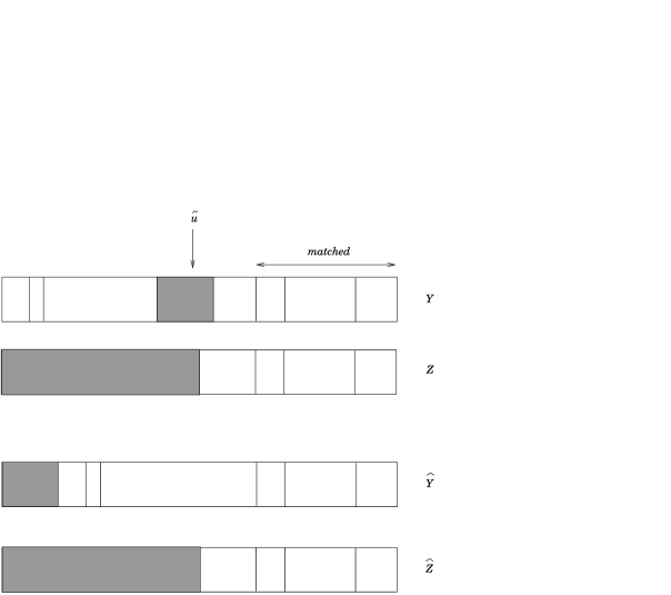
Figure 1: First step of the coupling. A point $\tilde{u}$ is uniformly chosen on $(0,1)$ and picks a part in $Y$ and $Z$, which are then rearranged into $\hat{Y},\hat{Z}$.

Let $a=|y|$ and let $b=|z|$ be the respective lengths of the pieces selected with $u$, and assume without loss of generality that $a<b$. Further rearrange, if needed, $y$ and $z$ so that after the rearrangement, $|u|=1/n$. Because $v\neq u$, necessarily $v>1/n$ (and is uniformly distributed on the set $\{2/n,\ldots,n/n\}$). The point $v$ designates a size-biased sample from the partition $\hat{Y}$ and we will construct another point $v^{\prime}$, which will also be uniformly distributed on $\{2/n,\ldots,n/n\}$, to similarly select a size-biased sample from $\hat{Z}$. However, while in the coupling of schramm one takes $v=v^{\prime}$, here we do not take them equal and apply to $v$ a measure-preserving map $\Phi$, defined as follows. Define the function

$$\Phi(x)=\cases{x,&\quad if $x>b$ or if $1/n\leq x\leq\gamma_{n}+1/n$,\cr x-\gamma_{n},&\quad if $a<x\leq b$,\cr x+b-a,&\quad if $\gamma_{n}+1/n<x\leq a$,}$$ (31)

where $\gamma_{n}:=\{(a-1/n)/2\}_{n}$. See Figure 2 for description of $\Phi$. Note that $\Phi$ is a measure-preserving map and hence $\tilde{v}^{\prime}:=\Phi(\tilde{v})$ is uniformly distributed on $(0,1)$. Define $v^{\prime}=\{\tilde{v}^{\prime}\}_{n}$. With $u,v$ and $v^{\prime}$ selected, the rest of the algorithm is unchanged, that is, we make the corresponding coagulations and fragmentations.

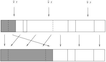
Figure 2: A second point $\tilde{v}$ is chosen uniformly in (0,1) and serves as a second size-biased pick for $\hat{Y}$. $\tilde{v}$ is mapped to $\tilde{v}^{\prime}=\Phi(\tilde{v})$ which gives a second size-biased pick for $\hat{Z}$.

This coupling has a number of remarkable properties which we summarize below. Essentially, the total number of unmatched entries can only decrease, and furthermore it is very difficult to create small unmatched entries, as the smallest unmatched entry can only become smaller by a factor of at most 2.

In what follows, we often speak of the “unmatched entries” between two permutations, meaning that we associate to these permutations elements of $\Omega_{n}$ and identify matched parts in $\Omega_{n}$ with matched cycles in the permutations. The translation between the two involves a factor $n$ concerning the size of the parts, and in all places it should be clear from the context whether we discuss parts in $\Omega_{n}$ or cycles of partitions.

Lemma 19

Let $U$ be the size of the smallest unmatched entry in two partitions $Y,Z\in\Omega_{n}$, let $Y^{\prime},Z^{\prime}$ be the corresponding partitions after one transposition of the coupling and let $U^{\prime}$ be the size of the smallest unmatched entry in $Y^{\prime},Z^{\prime}$. Assume that $2^{j}\leq U<2^{j+1}$ for some $j\geq 0$. Then it is always the case that $U^{\prime}\geq U-\{U/2\}_{n}$, and moreover,

$$\mathbb{P}(U^{\prime}\leq 2^{j})\leq 2^{j+2}/n.$$

Finally, the number of unmatched parts may only decrease.

Remark 20.

Since $U^{\prime}\,{\geq}\,U\,{-}\,\{U/2\}_{n}$, it holds in particular that $U^{\prime}\,{\geq}\,2^{j-1}$.

Proof of Lemma 19 That the number of unmatched entries can only decrease is similar to the proof of Lemma 3.1 in schramm . (In fact it is simpler here, since that lemma requires looking at the total number of unmatched entries of size greater than $\varepsilon$. Since in our discrete setup no entry can be smaller than $\varepsilon=1/n$ we do not have to take this precaution.) We continue to denote by $M_{j}$ the total number of parts in the range $[2^{j},2^{j+1})/n$. The only case that $U$ can decrease is if there is a fragmentation of an unmatched entry, since matched entries must fragment in exactly the same way. Now, note that the coupling is such that when an unmatched entry is selected and is fragmented, then all subsequent pieces are either greater or equal to $a-\{a/2\}_{n}$ (where $a$ is the size of the smaller of the two selected unmatched entries), or are matched. Moreover, for such a fragmentation to occur, one must select the lowest unmatched entry (this has probability at most $M_{j}2^{j+1}/n$, since there may be several unmatched entries with size $U$), and then fragment it, which has probability at most $2^{j+1}/n$, and thus $\mathbb{P}(U^{\prime}<U)\leq 4M_{j}4^{j}/n^{2}$. Since $M_{j}2^{j}\leq n$, this completes the proof.

We have described the basic step of a (random) transposition in the coupling. The step corresponding to a random $k$-cycle $\gamma=(\gamma_{1},\gamma_{2},\ldots,\gamma_{k})$ is obtained by taking $u_{1}=\gamma_{1}$, generating $v,v^{\prime}$ as in the coupling above (corresponding to the choice of $\gamma_{2}$), rearranging and taking $u_{2}$ to correspond to the location of $v,v^{\prime}$ after the rearrangement, drawing new $v,v^{\prime}$ (corresponding to $\gamma_{3}$) and so on. In doing so, we are disregarding the constraint that no repetitions are present in $\gamma$. However, as it turns out, we will be interested in an evolution lasting at most

$$\Delta:=n^{5/8}\log n,$$ (32)

and the expected number of times that a violation of this constraint occurs during this time is bounded by $2\Delta k^{2}/n$, which converges to $0$ as $n\to\infty$. Hence, we can in what follows disregard this violation of the constraint.

Now, start with two configurations $Y_{0},Z_{0}$ such that $Z_{0}$ is the element of $\Omega_{n}$ associated with a random uniform permutation. Assume also that initially, the small parts of $Y_{0}$ and $Z_{0}$ (i.e., those that are smaller than $K$, the closest dyadic integer to $\lfloor n^{\chi}\rfloor$), are exactly identical, and that they have the same parity. As we will now see, at time $\Delta$, $\pi_{t+\Delta}$ and $\pi^{\prime}_{\Delta}$ will be coupled, with high probability. Note also that, since initially all the parts that are smaller than $K$ are matched, the initial number of unmatched entries cannot exceed $n/K\leq n^{1/8}$, and this may only decrease with time by Lemma 19.

Lemma 21

In the next $\Delta$ units of time, the random permutation $\pi^{\prime}_{s}$ never has more than a fraction $n^{-1/8}(\log n)^{6}$ of the total mass in parts smaller than $n^{7/8}$, with high probability.

The proof is the same as that of Proposition 11, only simpler because the initial number of small clusters is within the required range. We omit further details. [This can also be seen by computing the probability that a given uniform permutation $\pi^{\prime}$ has more than a fraction $n^{-1/8}(\log n)^{6}$ of the total mass in parts smaller than $n^{7/8}$, and summing over $\operatorname{Poisson}(\Delta)$ steps.]

Lemma 22

In the next $\Delta$ units of time, every unmatched part of the permutations is greater than or equal to $n^{3/4}/2$, with high probability.

Recall that the total number of unmatched parts can never increase. Suppose the smallest unmatched part at time $s$ is of scale $j$ (i.e., of size in $[2^{j},2^{j+1})$), and let $j=U(s)$ be this scale. Then, when touching this part, the smallest scale it could go to is $j-1$, by the properties of the coupling (see Lemma 19). This happens with probability at most $2^{j+2}/n$. On the other hand, with the complementary probability, this part experiences a coagulation. And with reasonable probability, what it coagulates with is larger than itself, so that it will jump to scale $j+1$ or larger. To compute this probability, note that since this is the smallest unmatched part, all smaller parts are matched and thus have a total mass controlled by Lemma 21. In particular, on an event of high probability, this fraction of the total mass is at most $q:=n^{-1/8}(\log n)^{6}$. It follows that with probability at least $1-q$, the part jumps to scale at least $j+1$, and with probability at most $r_{j}:=2^{j+1}/n$, to scale $j-1$. Now, when this part jumps to scale at least $j+1$, this does not necessarily mean that the smallest unmatched part is in scale at least $j+1$, since there may be several small unmatched parts in scale $j$. However, there can never be more than $2n^{1/8}$ such parts. If an unmatched piece in scale $j$ is touched, we declare it a success if it moves to scale $j+1$ (which has probability at least $1-q$, given that it is touched) and a failure if it goes to scale $j-1$ (which has probability at most $r_{j}$). If $2n^{1/8}$ successes occur before any failure occurs at scale $j$, we say that a good success has occurred, and then we know that no unmatched cycle can exist at scale smaller than $j$. Call the complement of a good success a potential failure (which thus includes the cases of both a real failure and a success which is not good). The probability of a potential failure at scale $j$ is at most $2n^{1/8}r_{j}/(1-q+r_{j})$, which is bounded above by $p_{j}=6n^{1/8}2^{j}/n$.

Let $\{s_{i}\}_{i\geq 0}$ be the times at which the smallest unmatched part changes scale, with $s_{0}$ being the first time the smallest unmatched part is of scale $j_{0}$ where $2^{j_{0}}=n^{5/6}$. Let $\{U_{i}\}$ denote the scale of the smallest unmatched part at time $s_{i}$, and let $j_{1}$ be such that $2^{j_{1}}=n^{3/4}/2$. Introduce a birth–death chain on the integers, denoted $v_{n}$, such that $v_{0}=j_{0}$ and

$$\mathbb{P}(v_{n+1}=j-1|v_{n}=j)=\cases{1,&\quad if $j=j_{0}$,\cr 0,&\quad if $j=j_{1}$,\cr p_{j},&\quad otherwise,}$$ (33)

and

$$\quad\mathbb{P}(v_{n+1}=j+1|v_{n}=j)=\cases{1-\mathbb{P}(v_{n+1}=j-1|v_{n}=j),&\quad$j>j_{1}$,\cr 0,&\quad$j=j_{1}$.}$$ (34)

Set $\tau_{j}=\min\{n>0\dvtx v_{n}=j\}$, and an analysis of the birth–death chain defined by (33) and (34) gives that

$$\mathbb{P}^{j_{0}}(\tau_{j_{1}}<\tau_{j_{0}})=\frac{1}{\sum_{j=j_{1}+1}^{j_{0}}\prod_{m=j}^{j_{0}-1}(({1-p_{m}})/{p_{m}})}\leq\prod_{j=j_{1}+1}^{j_{0}-1}\frac{p_{j}}{1-p_{j}}$$

(see, e.g., Theorem (3.7) in Chapter 5 of durrett ). Thus $\mathbb{P}^{j_{0}}(\tau_{j_{1}}<\tau_{j_{0}})$ decays as an exponential in $(\log n)^{2}$. Therefore, since $\mathbb{P}(v_{2k\Delta}=j_{1})\leq 2k\Delta\mathbb{P}^{j_{0}}(\tau_{j_{1}}<\tau_{j_{0}})$, it follows that $\mathbb{P}(v_{2k\Delta}=j_{1})\to 0$ as $n\to\infty$. On the other hand, between times $t$ and $t+\Delta$, the process $\{U_{i}\}_{i\geq 1}$ may have made at most $2k\Delta$ moves with overwhelming probability. This implies that $U_{i}\geq j_{1}$ with high probability throughout $[t,t+\Delta]$.

End of the proof of Theorem 1. We now are going to prove that, after $\Delta=n^{5/8}\log n$ steps, there are no more unmatched parts with high probability. The basic idea is that, on the one hand, the number of unmatched parts may never increase, and on the other hand, it does decrease frequently enough. Since each unmatched part is greater than $n^{3/4}/2$ during this time, any given pair of unmatched parts is merging at rate roughly $n^{-1/2}$. There are initially no more than $2n^{1/8}$ unmatched parts, so after $n^{5/8}\log n=\Delta$ steps, no more unmatched part remains with high probability.

To be precise, assume that there are $L$ unmatched parts. Let $T_{L}$ be the time to decrease the number of unmatched parts from $L$ to $L-2$. Observe that, for parity reasons ($\pi$ and $\pi^{\prime}$ must have the same parity of number of parts at all times), $L$ is always even. Note also that $L=2$ is impossible, so $L$ is at least 4. Assume to start with that both copies have at least 2 unmatched parts. Then, at rate greater than $n^{-1/4}/2$ we pick an unmatched part in the first point $u_{1}$ for the $k$-cycle. Since there are at least 2 unmatched parts in each copy, let $R$ be the interval of $(0,1)$ corresponding to a second unmatched part in the copy that contains the larger of the two selected ones. Then $|R|>n^{-1/4}/2$, and moreover when $v$ falls in $R$, we are guaranteed that a coagulation is going to occur in both copies. We interpret this event as a success, and declare every other possibility a failure. Hence if $G$ is a geometric random variable with success probability $n^{-1/4}/2$, and $(X_{j})_{j=1}^{\infty}$ are i.i.d. exponentials with mean $2n^{1/4}$, the total amount of time before a success occurs is dominated by $\sum_{j=1}^{G}X_{j}$.

If, however, one copy (say $\pi$) has only one unmatched part, then one first has to break that component, which takes at most an exponential random variable with rate $n^{-1/2}/4$. Note that the other copy must have had at least 3 unmatched parts, so after breaking the big one, both copies have now at least two unmatched copies and we are back to the preceding case. It follows from this analysis that in any case, $T_{L}$ is dominated by

$$T_{L}\preceq Y+\sum_{j=1}^{G}X_{j}\vspace*{3pt}$$

and so $\mathbb{E}(T_{L})\leq 4n^{1/2}+4n^{1/2}=8n^{1/2}$. Now, let

$$\tau_{L}=T_{L}+T_{L-2}+\cdots+T_{4}\vspace*{3pt}$$

and let $T=\tau_{2n^{1/8}}$. Then $T$ is the time to get rid of all unmatched parts. We obtain from the above $\mathbb{E}(T)\leq 16n^{5/8}$. By Markov’s inequality, it follows that $T<n^{5/8}\log n=\Delta$ with high probability. This concludes the proof of Theorem 1.

References

- (1) {bincollection}[mr] \bauthor\bsnmAldous, \bfnmDavid\binitsD. (\byear1983). \btitleRandom walks on finite groups and rapidly mixing Markov chains. In \bbooktitleSeminar on Probability, XVII. \bseriesLecture Notes in Math. \bvolume986 \bpages243–297. \bpublisherSpringer, \baddressBerlin. \bidmr=0770418 \endbibitem
- (2) {bbook}[mr] \bauthor\bsnmArratia, \bfnmRichard\binitsR., \bauthor\bsnmBarbour, \bfnmA. D.\binitsA. D. and \bauthor\bsnmTavaré, \bfnmSimon\binitsS. (\byear2003). \btitleLogarithmic Combinatorial Structures: A Probabilistic Approach. \bpublisherEur. Math. Soc., \baddressZürich. \biddoi=10.4171/000, mr=2032426 \endbibitem
- (3) {barticle}[mr] \bauthor\bsnmArratia, \bfnmRichard\binitsR. and \bauthor\bsnmTavaré, \bfnmSimon\binitsS. (\byear1992). \btitleThe cycle structure of random permutations. \bjournalAnn. Probab. \bvolume20 \bpages1567–1591. \bidmr=1175278 \endbibitem
- (4) {barticle}[mr] \bauthor\bsnmBarbour, \bfnmA.\binitsA. (\byear1990). \btitleComments on “Poisson approximations and the Chen–Stein method,” by R. Arratia, L. Goldstein and L. Gordon. \bjournalStatist. Sci. \bvolume5 \bpages425–427. \endbibitem
- (5) {barticle}[mr] \bauthor\bsnmBerestycki, \bfnmNathanaël\binitsN. and \bauthor\bsnmDurrett, \bfnmRick\binitsR. (\byear2006). \btitleA phase transition in the random transposition random walk. \bjournalProbab. Theory Related Fields \bvolume136 \bpages203–233. \biddoi=10.1007/s00440-005-0479-7, mr=2240787 \endbibitem
- (6) {bbook}[mr] \bauthor\bsnmDiaconis, \bfnmPersi\binitsP. (\byear1988). \btitleGroup Representations in Probability and Statistics. \bseriesInstitute of Mathematical Statistics Lecture Notes—Monograph Series \bvolume11. \bpublisherIMS, \baddressHayward, CA. \bidmr=0964069 \endbibitem
- (7) {barticle}[mr] \bauthor\bsnmDiaconis, \bfnmPersi\binitsP. and \bauthor\bsnmShahshahani, \bfnmMehrdad\binitsM. (\byear1981). \btitleGenerating a random permutation with random transpositions. \bjournalZ. Wahrsch. Verw. Gebiete \bvolume57 \bpages159–179. \biddoi=10.1007/BF00535487, mr=0626813 \endbibitem
- (8) {bbook}[mr] \bauthor\bsnmDurrett, \bfnmRichard\binitsR. (\byear2004). \btitleProbability: Theory and Examples, \bedition3rd ed. \bpublisherDuxbury Press, \baddressBelmont, CA. \endbibitem
- (9) {barticle}[mr] \bauthor\bsnmFlatto, \bfnmL.\binitsL., \bauthor\bsnmOdlyzko, \bfnmA. M.\binitsA. M. and \bauthor\bsnmWales, \bfnmD. B.\binitsD. B. (\byear1985). \btitleRandom shuffles and group representations. \bjournalAnn. Probab. \bvolume13 \bpages154–178. \bidmr=0770635 \endbibitem
- (10) {barticle}[mr] \bauthor\bsnmKaroński, \bfnmMichał\binitsM. and \bauthor\bsnmŁuczak, \bfnmTomasz\binitsT. (\byear1997). \btitleThe number of connected sparsely edged uniform hypergraphs. \bjournalDiscrete Math. \bvolume171 \bpages153–167. \biddoi=10.1016/S0012-365X(96)00076-3, mr=1454447 \endbibitem
- (11) {bbook}[mr] \bauthor\bsnmLevin, \bfnmDavid A.\binitsD. A., \bauthor\bsnmPeres, \bfnmYuval\binitsY. and \bauthor\bsnmWilmer, \bfnmElizabeth L.\binitsE. L. (\byear2009). \btitleMarkov Chains and Mixing Times. \bpublisherAmer. Math. Soc., \baddressProvidence, RI. \bidmr=2466937 \endbibitem
- (12) {barticle}[mr] \bauthor\bsnmLulov, \bfnmNathan\binitsN. and \bauthor\bsnmPak, \bfnmIgor\binitsI. (\byear2002). \btitleRapidly mixing random walks and bounds on characters of the symmetric group. \bjournalJ. Algebraic Combin. \bvolume16 \bpages151–163. \biddoi=10.1023/A:1021172928478, mr=1943586 \endbibitem
- (13) {bbook}[mr] \bauthor\bsnmLulov, \bfnmNathan Anton Mikerin\binitsN. A. M. (\byear1996). \btitleRandom Walks on the Symmetric Group Generated by Conjugacy Classes. \bpublisherProQuest LLC, \baddressAnn Arbor, MI. \bnoteThesis (Ph.D.)–Harvard Univ. \bidmr=2695111 \endbibitem
- (14) {bincollection}[auto:STB—2010-11-18—09:18:59] \bauthor\bsnmRoichman, \bfnmY.\binitsY. (\byear1999). \btitleCharacters of the symmetric group: Formulas, estimates, and applications. In \bbooktitleEmerging Applications of Number Theory (\beditorD. A. Hejhal, \beditorJ. Friedman, \beditorM. C. Gutzwiller and \beditorA. M. Odlyzko, eds.). \bseriesIMA Volumes on Applied Mathematics \bvolume109 \bpages525–545. \bpublisherSpringer, \baddressNew York. \endbibitem
- (15) {barticle}[mr] \bauthor\bsnmRoichman, \bfnmYuval\binitsY. (\byear1996). \btitleUpper bound on the characters of the symmetric groups. \bjournalInvent. Math. \bvolume125 \bpages451–485. \biddoi=10.1007/s002220050083, mr=1400314 \endbibitem
- (16) {bmisc}[auto:STB—2010-11-18—09:18:59] \bauthor\bsnmRoussel, \bfnmS.\binitsS. (\byear1999). \bhowpublishedMarches aléatoires sur e groupe symétrique. Thèse de doctorat, Toulouse. \endbibitem
- (17) {barticle}[mr] \bauthor\bsnmRoussel, \bfnmSandrine\binitsS. (\byear2000). \btitlePhénomène de cutoff pour certaines marches aléatoires sur le groupe symétrique. \bjournalColloq. Math. \bvolume86 \bpages111–135. \bidmr=1799892 \endbibitem
- (18) {bincollection}[mr] \bauthor\bsnmSaloff-Coste, \bfnmLaurent\binitsL. (\byear2004). \btitleRandom walks on finite groups. In \bbooktitleProbability on Discrete Structures. \bseriesEncyclopaedia Math. Sci. \bvolume110 \bpages263–346. \bpublisherSpringer, \baddressBerlin. \bidmr=2023654 \endbibitem
- (19) {barticle}[mr] \bauthor\bsnmSaloff-Coste, \bfnmL.\binitsL. and \bauthor\bsnmZúñiga, \bfnmJ.\binitsJ. (\byear2008). \btitleRefined estimates for some basic random walks on the symmetric and alternating groups. \bjournalALEA Lat. Am. J. Probab. Math. Stat. \bvolume4 \bpages359–392. \bidmr=2461789 \endbibitem
- (20) {barticle}[mr] \bauthor\bsnmSchramm, \bfnmOded\binitsO. (\byear2005). \btitleCompositions of random transpositions. \bjournalIsrael J. Math. \bvolume147 \bpages221–243. \biddoi=10.1007/BF02785366, mr=2166362 \endbibitem
- (21) {barticle}[mr] \bauthor\bsnmVershik, \bfnmA. M.\binitsA. M. and \bauthor\bsnmKerov, \bfnmS. V.\binitsS. V. (\byear1981). \btitleAsymptotic theory of the characters of a symmetric group. \bjournalFunktsional. Anal. i Prilozhen. \bvolume15 \bpages15–27 \bnote(in Russian). \bidmr=0639197 \endbibitem