Dissipative Taylor-Couette flows under the influence of helical magnetic fields

Abstract

The linear stability of MHD Taylor-Couette flows in axially unbounded cylinders is considered, for magnetic Prandtl number unity. Magnetic fields varying from purely axial to purely azimuthal are imposed, with a general helical field parameterized by $\beta=B_{\phi}/B_{z}$. We map out the transition from the standard MRI for $\beta=0$ to the nonaxisymmetric Azimuthal MagnetoRotational Instability (AMRI) for $\beta\to\infty$. For finite $\beta$, positive and negative wave numbers $m$, corresponding to right and left spirals, are no longer identical. The transition from $\beta=0$ to $\beta\to\infty$ includes all the possible forms of MRI with axisymmetric and nonaxisymmetric modes. For the nonaxisymmetric modes, the most unstable mode spirals in the opposite direction to the background field. The standard ($\beta=0$) MRI is axisymmetric for weak fields (including the instability with the lowest Reynolds number) but is nonaxisymmetric for stronger fields.

If the azimuthal field is due in part to an axial current flowing through the fluid itself (and not just along the central axis), then it is also unstable to the nonaxisymmetric Tayler instability, which is most effective without rotation. For large $\beta$ this instability has wavenumber $m=1$, whereas for $\beta\simeq 1$ $m=2$ is most unstable. The most unstable mode spirals in the same direction as the background field.

I Introduction

The longstanding problem of the generation of turbulence in various hydrodynamically stable situations has found a solution in recent years with the MHD shear flow instability, the so-called magnetorotational instability (MRI), in which the presence of a magnetic field has a destabilizing effect on a differentially rotating flow with outward decreasing angular velocity but increasing angular momentum BH91 ; V59 .

In the absence of MHD effects, according to the Rayleigh criterion, an ideal flow is stable against axisymmetric perturbations whenever the specific angular momentum increases outward

$$\frac{{\rm{d}}}{{\rm{d}}R}(R^{2}\Omega)^{2}>0,$$ (1)

where $\Omega$ is the angular velocity, and ($R$, $\phi$, $z$) are cylindrical coordinates. In the presence of an azimuthal magnetic field $B_{\phi}$, this criterion is modified to

$$\frac{1}{R^{3}}\frac{{\rm{d}}}{{\rm{d}}R}(R^{2}\Omega)^{2}-\frac{R}{\mu_{0}\rho}\frac{{\rm{d}}}{{\rm{d}}R}\left(\frac{B_{\phi}}{R}\right)^{2}>0,$$ (2)

where $\mu_{0}$ is the permeability and $\rho$ the density M54 . Note also that this criterion is both necessary and sufficient for (axisymmetric) stability. In particular, all ideal flows can thus be destabilized, by azimuthal magnetic fields with the right profiles and amplitudes.

On the other hand, for nonaxisymmetric modes, one has

$$\frac{{\rm{d}}}{{\rm{d}}R}(RB_{\phi}^{2})<0$$ (3)

as the necessary and sufficient condition for stability of an ideal fluid at rest T73 . Outwardly increasing fields are therefore unstable. If (3) is violated, the most unstable mode has azimuthal wavenumber $m=1$.

The rich variety of nonaxisymmetric instabilities can be demonstrated by the addition of a differential rotation. In this case even the current-free (within the fluid) profile $B_{\phi}\propto 1/R$ (which according to (3) is stable for $\Omega=0$) can become unstable. Even for a differential rotation that by itself would be stable according to 1, the combination of $\Omega$ and $B_{\phi}\propto 1/R$ can be unstable to $m=1$ perturbations (see Fig. 2). We have called this phenomenon the Azimuthal MagnetoRotational Instability (AMRI). It has even been demonstrated that it should be possible to observe the AMRI in laboratory experiments, H09 .

Further new phenomena appear if an axial field is added, yielding a spiral, or helical total field. In this case only a sufficient condition for stability against axisymmetric perturbations is known. In the absence of rotation this is

$$\frac{d}{dR}(R^{2}B_{\phi}^{2})<0,$$ (4)

(see also Eq. (6)). Including rotation, this was extended HG62 to

$$R\frac{d\Omega^{2}}{dR}-\frac{1}{\mu_{0}\rho R^{3}}\frac{d}{dR}(RB_{\phi})^{2}>0.$$ (5)

For the current-free field $B_{\phi}\propto 1/R$, only superrotating flows with ${\rm d}\Omega/{\rm d}R>0$ are stable. Indeed, we have demonstrated that dissipative Taylor-Couette flows beyond the Rayleigh limit for centrifugal instability can easily be destabilized by helical magnetic fields with such a current-free azimuthal component HR05 . The resulting axisymmetric traveling wave instability has become known as the Helical MagnetoRotational Instability (HMRI), and has been obtained in the PROMISE experiment R06 ; St06 .

In the PROMISE experiment the azimuthal field is $B_{\phi}\propto 1/R$. In this paper we will also consider the generalization to $B_{\phi}=a_{B}R+b_{B}/R$, where the extra term $a_{B}R$ corresponds to an axial electric current running through the fluid as well, and hence opens the possibility of current-induced (Tayler) instabilities. The resulting (nonaxisymmetric) instabilities may also be modified by adding either a differential rotation or an axial magnetic field.

One might suppose that adding an axial field would be important only if its amplitude is of the same order as that of the azimuthal field. Chandrasekhar C61 showed that for $\Omega=0$, a sufficiently strong axial field will always suppress any axisymmetric instabilities of an azimuthal field, by deriving the stability condition

$$IB^{2}_{z}>\int\frac{\xi_{R}^{2}}{R^{2}}\frac{{\rm d}}{{\rm d}R}(R^{2}B_{\phi}^{2})\ \ {\rm d}R,$$ (6)

where $I>0$ and $\xi_{R}$ is the (purely real) radial eigenfunctions. (Note how (6) reduces to (4) for $B_{z}=0$.) However, we will show that the influence of $B_{z}$ cannot be ignored even for rather small values.

We will find that, depending on the magnitudes of the imposed differential rotation and magnetic fields, the field may either stabilize or destabilize the differential rotation, and the most unstable mode may be either the axisymmetric Taylor vortex flow (the SMRI or HMRI), or the nonaxisymmetric AMRI, or the nonaxisymmetric Tayler instability. In combined axial and azimuthal fields, we will also show that the nonaxisymmetric modes differ between $m$ and $-m$, corresponding to left and right spirals. As first pointed out by K96 , if the imposed field has both axial and azimuthal components, the system no longer exhibits $\pm z$ symmetry. For axisymmetric modes, the consequence of this is that what were previously stationary modes (SMRI) become oscillatory, traveling wave modes (HMRI). For nonaxisymmetric modes, breaking the $\pm z$ symmetry of the basic state breaks the $\pm m$ symmetry of the instabilities. Physically this corresponds to the fact that modes spiraling either in the same or the opposite sense to the spiral structure of the basic state are indeed different. This $\pm m$ symmetry breaking is also a convenient distinguishing feature between the AMRI and the Tayler instabilities; for the AMRI the most unstable mode spirals in the opposite sense to the imposed field, for the Tayler instabilities in the same sense.

Finally, in order to produce benchmarks for the application of incompressible 3D MHD codes, in this work we will focus primarily on magnetic Prandtl number ${\rm Pm}=1$.

II The equations

We are interested in the linear stability of the background field $\mbox{\boldmath$B$}=(0,B_{\phi}(R),B_{0})$, with $B_{0}=$const, and the flow $\mbox{\boldmath$U$}=(0,R\Omega(R),0)$. The perturbed state of the system is described by

$$u_{R},\ u_{\phi},\ u_{z},\ p,\ b_{R},\ b_{\phi},\ b_{z}.$$ (7)

Developing the disturbances into normal modes, the solutions of the linearized MHD equations are considered in the form

$$F=F(R){\rm exp}({\rm i}(kz+m\phi+\omega t)),$$ (8)

where $F$ is any of the velocity, pressure, or magnetic field disturbances.

The governing equations are

$$\frac{\partial\mbox{\boldmath$u$}}{\partial t}+(\mbox{\boldmath$U$}\cdot\nabla)\mbox{\boldmath$u$}+(\mbox{\boldmath$u$}\cdot\nabla)\mbox{\boldmath$U$}=-\frac{1}{\rho}\nabla p+\nu\Delta\mbox{\boldmath$u$}+$$ (9)

$$+\frac{1}{\mu_{0}\rho}{\rm curl}\ \mbox{\boldmath$b$}\times\mbox{\boldmath$B$}+\frac{1}{\mu_{0}\rho}{\rm curl}\ \mbox{\boldmath$B$}\times\mbox{\boldmath$b$},$$ (10)

$$\frac{\partial\mbox{\boldmath$b$}}{\partial t}={\rm curl}(\mbox{\boldmath$u$}\times\mbox{\boldmath$B$})+{\rm curl}(\mbox{\boldmath$U$}\times\mbox{\boldmath$b$})+\eta\Delta\mbox{\boldmath$b$},$$ (11)

and

$${\rm div}\ \mbox{\boldmath$u$}={\rm div}\ \mbox{\boldmath$b$}=0,$$ (12)

where $u$ is the perturbed velocity, $b$ the magnetic field, $p$ the pressure perturbation. $\nu$ is the kinematic viscosity and $\eta$ the magnetic diffusivity.

Figure 1: The basic state azimuthal field with prescribed values at the inner and outer cylinders.

The stationary background solution is

$$\Omega=a_{\Omega}+\frac{b_{\Omega}}{R^{2}},\ \ \ \ \ B_{\phi}=a_{B}R+\frac{b_{B}}{R},$$ (13)

where $a_{\Omega}$, $b_{\Omega}$, $a_{B}$ and $b_{B}$ are constants defined by

$$a_{\Omega}=\Omega_{\rm{in}}\frac{\mu_{\Omega}-{\hat{\eta}}^{2}}{1-{\hat{\eta}}^{2}},\qquad b_{\Omega}=\Omega_{\rm{in}}R_{\rm{in}}^{2}\frac{1-\mu_{\Omega}}{1-{\hat{\eta}}^{2}},$$

$$a_{B}=\frac{B_{\rm{in}}}{R_{\rm{in}}}\frac{\hat{\eta}(\mu_{B}-\hat{\eta})}{1-\hat{\eta}^{2}},\qquad b_{B}=B_{\rm{in}}R_{\rm{in}}\frac{1-\mu_{B}\hat{\eta}}{1-\hat{\eta}^{2}},$$ (14)

with

$$\hat{\eta}=\frac{R_{\rm{in}}}{R_{\rm{out}}},\;\;\;\mu_{\Omega}=\frac{\Omega_{\rm{out}}}{\Omega_{\rm{in}}},\;\;\;\mu_{B}=\frac{B_{\rm{out}}}{B_{\rm{in}}}.$$ (15)

$R_{\rm{in}}$ and $R_{\rm{out}}$ are the radii of the inner and outer cylinders, $\Omega_{\rm{in}}$ and $\Omega_{\rm{out}}$ are their rotation rates, and $B_{\rm{in}}$ and $B_{\rm{out}}$ the azimuthal magnetic fields at the inner and outer cylinders. The possible magnetic field solutions are plotted in Fig. 1. Note that – unlike $\Omega$, where $\Omega_{\rm{in}}$ and $\Omega_{\rm{out}}$ are the physically relevant quantities – for $B_{\phi}$ the fundamental quantities are not so much $B_{\rm{in}}$ and $B_{\rm{out}}$, but rather $a_{B}$ and $b_{B}$ themselves. In particular, a field of the form $b_{B}/R$ is generated by running an axial current only through the inner region $R<R_{\rm{in}}$, whereas a field of the form $a_{B}R$ is generated by running a uniform axial current through the entire region $R<R_{\rm{out}}$, including the fluid.

Given the $z$-component of the electric current, ${\rm curl}_{z}\mbox{\boldmath$B$}=2a_{B}$, one finds for the current helicity of the background field

$${\rm curl}\mbox{\boldmath$B$}\cdot\mbox{\boldmath$B$}=2a_{B}B_{0},$$ (16)

which may be either positive or negative (and of course vanishes for the current-free case $a_{B}=0$). However, both signs yield the same instability curves, merely with the previously mentioned left and right spirals interchanged.

The inner value $B_{\rm in}$ is normalized with the uniform vertical field, i.e.

$$\beta=\frac{B_{\rm in}}{B_{0}}.$$ (17)

For $\mu_{B}=1$ we have

$${\rm curl}\mbox{\boldmath$B$}\cdot\mbox{\boldmath$B$}=\frac{2\beta}{3}\frac{B_{0}^{2}}{R_{\rm in}}.$$ (18)

The sign of $\beta$ thus determines the sign of the helicity of the background field. And again, interchanging $\pm\beta$ simply interchanges left and right spirals $\pm m$.

As usual, the toroidal field amplitude is measured by the Hartmann number

$${\rm Ha}=\frac{B_{\rm in}R_{0}}{\sqrt{\mu_{0}\rho\nu\eta}}.$$ (19)

$R_{0}=\sqrt{R_{\rm in}(R_{\rm out}-R_{\rm in})}$ is used as the unit of length, $\eta/R_{0}$ as the unit of velocity and $B_{\rm in}$ as the unit of the azimuthal fields. Frequencies, including the rotation $\Omega$, are normalized with the inner rotation rate $\Omega_{\rm in}$. The magnetic Reynolds number Rm is defined as

$${\rm Rm}=\frac{\Omega_{\rm in}R_{0}^{2}}{\eta}.$$ (20)

The Lundquist number S is defined by $\rm S=Ha\cdot\sqrt{Pm}$.

The boundary conditions associated with the perturbation equations are no-slip for $u$,

$$u_{R}=u_{\phi}=u_{z}=0,$$ (21)

and perfectly conducting for $b$,

$$db_{\phi}/dR+b_{\phi}/R=b_{R}=0.$$ (22)

These boundary conditions hold for both $R=R_{\rm{in}}$ and $R=R_{\rm{out}}$.

If we consider a constant phase of a nonaxisymmetric pattern, Eq. (8) yields

$$\frac{\partial z}{\partial t}\bigg{|}_{\phi}=-\frac{\Re(\omega)}{k},\ \ \ \ \ \ \ \ \ \frac{\partial\phi}{\partial t}\bigg{|}_{z}=-\frac{\Re(\omega)}{m}.$$ (23)

The first relation describes the phase velocity of the modes in the axial direction, the second in the azimuthal direction (and only exists for nonaxisymmetric modes). Obviously the wave is traveling upwards if the real part of the eigenfrequency is negative.

At a fixed time the phase relations (23) can also be written as

$$\partial z/\partial\phi=-m/k.$$ (24)

Now, $k$ and $m$ are both real numbers, and without loss of generality one of them can be taken to be positive, say $k$. The other one, $m$ in this case, must be allowed to have both signs though. Negative $m$ describe right-hand spirals (marked here by R), and positive $m$ describe left-hand spirals (marked here by L). If the axisymmetric background field possesses positive $B_{z}$ and $B_{\phi}$ (as used for the calculations here) then its current helicity is positive, or equivalently, it forms a right spiral.

III From AMRI to HMRI

We begin with a purely azimuthal field, and no electric currents within the fluid, that is, $B_{\phi}\propto 1/R$. Figure 2 presents results for $\mu_{\Omega}=0.5$, showing that for $\rm Ha>100$ and $\rm Re>200$ there exists an $m=1$ nonaxisymmetric instability. Note also how both the upper and lower branches of the instability curve tilt to the right, that is, have a positive slope $d{\rm Re}/d{\rm Ha}$. For a given Hartmann number, the instability therefore only exists within a finite range of Reynolds numbers. If $\rm Re$ is too large, the instability disappears again as a consequence of the suppressing action that differential rotation often has on nonaxisymmetric modes.

Figure 2: Azimuthal MagnetoRotational Instability (AMRI): The instability curve for current-free azimuthal magnetic fields. The most unstable mode is nonaxisymmetric, with $m=1$. Axisymmetric instabilities do not exist at all in this configuration. $\mu_{B}=0.5$, $\mu_{\Omega}=0.5$. $\rm Pm=1$.

We consider next a purely axial field, the so-called standard MRI. In this case both axisymmetric and nonaxisymmetric modes may be excited, with the axisymmetric mode being the one with the overall lowest Reynolds number (Fig. 3). For $\rm Pm=1$ this overall minimum occurs for $\rm Ha\simeq 10$ and $\rm Re\simeq 80$. However, for sufficiently large $\rm Ha$ the $m=1$ nonaxisymmetric mode is actually preferred over the axisymmetric mode. The standard MRI for purely axial fields is therefore not necessarily an axisymmetric mode. The axisymmetric mode only dominates for sufficiently weak fields, including also the global minimum $\rm Re$ value. It also dominates the entire weak-field branch of the instability curves (Fig. 3). The axisymmetric mode here tilts to the left, whereas the nonaxisymmetric mode tilts to the right, as before in Fig. 2.

Figure 3: Standard MRI: The instability curves for uniform axial magnetic fields. For ${\rm Ha}<75$ the axisymmetric mode is preferred; for ${\rm Ha}>75$ the $m=1$ nonaxisymmetric mode is preferred. The global minimum $\rm Re$ value is for the axisymmetric mode. $\mu_{\Omega}=0.5$, $\rm Pm=1$.

Figure 4 finally shows results combining azimuthal and axial fields, focusing in this case on $\beta=2$ (so a right-handed helicity). We see the same general pattern as before: only the weak-field branch of the $m=0$ mode tilts to the left; all nonaxisymmetric modes tilt to the right. Up to ${\rm Ha}\approx 50$ the axisymmetric mode is preferred, just as before for the standard MRI. For ${\rm Ha}>50$ the $m=1$ right spiral is preferred.

Figure 4 also demonstrates that the (axisymmetric) standard MRI and the (nonaxisymmetric) AMRI are the basic elements which both appear, with different weights, if the background field has a spiral geometry. From this point of view instabilities in helical fields are simply a mixture of these two basic elements. More specifically, one finds that the weak-field branch of the instability in Fig. 4 is very similar to the weak-field branch of the standard MRI (Fig. 3) while the strong-field branch strongly resembles the strong-field branch of AMRI (Fig. 2). The minimum is always obtained for the axisymmetric mode of the standard MRI. The only difference between the standard MRI and HMRI is the different character of the eigenfrequencies: the SMRI is stationary, whereas the HMRI is oscillatory, as a necessary consequence of the $\pm z$ symmetry-breaking K96 . It is precisely this oscillatory nature of the HMRI that has been used to identify it in the PROMISE experiment R06 ; St06 .

Figure 4: Helical magnetorotational instability (HMRI): The instability curves for current-free ($\mu_{B}=0.5$) helical fields with $\beta=2$. $\mu_{\Omega}=0.5$. The dotted line gives the axisymmetric mode. The solid lines are marked with the mode number $m$ and the type of helicity (L left, R right). Note that for stronger fields the most unstable mode is nonaxisymmetric with the same helicity as the helicity of the background field. The mode with the lowest Re is always axisymmetric. Top: $\rm Pm=1$, bottom: $\rm Pm=0.01$.

Note finally that taking $\rm Pm=1$ greatly simplifies the results, and indeed eliminates some particularly interesting results. As we have previously demonstrated, both the (axisymmetric) HMRI HR05 as well as the (nonaxisymmetric) AMRI H09 have the property that their scalings with Pm vary dramatically with $\mu_{\Omega}$. For $\mu_{\Omega}$ only somewhat greater than the Rayleigh value, both modes have Ha and Re as the relevant measures of field strength and rotation rates, whereas for greater values of $\mu_{\Omega}$, $\rm S=Ha\cdot\sqrt{Pm}$ and $\rm Rm=Re\cdot Pm$ are the relevant measures. For small Pm the differences can thus be huge. Insulating versus conducting boundaries can also have a surprisingly large influence on this transition from one scaling to another RH07 .

IV Fields with current-helicity

IV.1 Steep rotation law

Figure 5: Tayler instability (TI) of a toroidal field under the influence of differential rotation with stationary outer cylinder. The solid curve is $m=1$, the dotted curve is $m=0$. $\mu_{B}=1$, $\mu_{\Omega}=0$. $\rm Pm=1$.

We begin by considering the stability of purely toroidal fields, and differential rotation profiles with a stationary outer cylinder. There are then three classical results known: First, in the absence of any fields, axisymmetric Taylor vortices arise at $\rm Re=68$, and nonaxisymmetric instabilities at $\rm Re=75$. Second, in the absence of any rotation, $m=1$ Tayler instabilities arise at $\rm Ha=150$. Figure 5 shows how these results are linked when both Ha and Re are non-zero. For Ha very small, the axisymmetric Taylor vortex mode is stabilized, whereas the nonaxisymmetric mode is eventually destabilized, and connects smoothly to the pure Tayler instability.

Figure 6: Instability curves for magnetic fields with positive current helicity. The curves are marked with their azimuthal wave numbers $m$. The shaded areas are the stable regions. Without magnetic fields the curves always start at $\rm Re=68$ for the $m=0$ Taylor vortices. Note the dominance of the axisymmetric modes (dotted) also for weak magnetic fields, unless for very high $\beta$ the field becomes nearly toroidal. $\rm Pm=1$, $\mu_{B}=1$, $\mu_{\Omega}=0$.

The next step is to add a uniform axial field to the azimuthal field, with (say) positive polarity. The background field then has a positive helicity, that is, it spirals to the right. If the axial field is weak, e.g. with $\beta=100$, then the marginal instability curves (Fig. 6, top) strongly resemble the map for $\beta\to\infty$ (Fig. 5). The main differences are i) the slightly smaller Hartmann number of the toroidal field, and ii) the splitting of the spiral modes $m=1$ and $m=-1$ into two curves with different helicity (R and L). The left-hand modes require a greater rotation than the right-hand modes. For background fields with positive helicity, we thus find that the right spirals are preferred, whereas for background fields with negative helicity, R and L would be exchanged, and the left spirals would be preferred.

For $\beta=10$ the differences between the L and R modes for given $m$ increase, so that the pure Tayler instability exists only as the 1R mode. The 1L mode no longer connects to $\rm Re=0$, and is not the most unstable mode anywhere in the given domain (Fig. 6, middle).

The 1R mode also dominates for $\beta$ of order unity. There is, however, an interesting particularity in this case. For very slow rotation, a 2R mode reduces the stability domain. For $\rm Re\simeq 0$, and in a limited range of Ha ($\rm Ha\simeq 100...130$), this mode forms the first instability (see BU08 ). A small amount of differential rotation, however, brings the system back to the 1R instability.

For models with helical fields and steep rotation laws (with stationary outer cylinder), we indeed find the expected splitting between right and left spiral instabilities. If the axisymmetric background field is right-handed, then the first unstable mode is also right-handed. The corresponding critical magnetic field strength is reduced compared to the TI of purely toroidal fields. If both magnetic field components are of the same order then the 2R mode is found to destabilize the system at the strong-field side of the stability domain, but only for very slow rotation. The differential rotation basically limits the action of this 2R mode.

IV.2 Flat rotation law

For weak magnetic fields and the steep rotation law, the axisymmetric Taylor vortex mode is the most easily excited instability. For a sufficiently flat rotation law the non-magnetic Taylor vortices necessarily disappear, and a critical Reynolds number no longer exists for $\rm Ha=0$. For the flat rotation law with $\mu_{\Omega}=0.5$, and the nearly uniform toroidal field with $\mu_{B}=1$, the instability curves for purely toroidal fields are given by Fig. 7. Both of the previous instabilities appear in this case: TI exists in the lower right corner, and AMRI exists in the upper left corner. The AMRI arises from the term $b_{B}/R$ in the magnetic background field profile (13), while the current-driven TI is due to the term $a_{B}R$. The two instabilities are separated by a stable branch with ${\rm Re}\approx{\rm Ha}$, where the differential rotation stabilizes the TI.

Figure 7: Flat rotation law ($\mu_{\Omega}=0.5$) and $B_{z}=0$. The curves are marked with their mode number $m$. The AMRI occurs in the upper left corner, and the TI in the lower right corner. $\mu_{B}=1$, $\rm Pm=1$

Figure 8: The same as in Fig. 7 but for finite values of $\beta$: Left: $\beta=100$ (top) and $\beta=10$ (bottom), Right: $\beta=2$ (top) and $\beta=0.1$ (bottom). The curves are marked with the azimuthal mode numbers $m$, the curves for $m=0$ are dotted. The notation R (right spiral) stands for negative $m$ and the notation L (left spiral) stands for positive $m$, It is $\mu_{B}=1$, $\rm Pm=1$.

For $\beta=\infty$ the modes with positive and negative $m$ are degenerate. At the weak-field limit the line for $m=2$ even crosses the line for $m=1$. Nevertheless, the AMRI solution with the lowest Reynolds number is a nonaxisymmetric mode with $m=1$. We find that this remains true for helical background fields with large $\beta$, but for $\beta$ of order unity and smaller the $m=0$ mode yields the instability with the lowest Reynolds number (Fig. 8) – as is also true for the standard MRI and HMRI. The transition from nonaxisymmetry to axisymmetry can be accomplished simply by increasing the axial component of the background field. It is thus clear that there is a smooth transition from one form of the MRI in TC flows to the next. The same is true for the corresponding eigenfrequencies, which develop from real values (for standard MRI) to complex values (in all other cases).

Figure 9: The critical Hartmann number (19) for $m=-1\dots-5$ and $\beta\lower 1.72218pt\hbox{$\;\buildrel<\over{\scriptstyle\sim}\;$}10$. An increasing dominance of the axial magnetic field component acts stabilizing. The curves do not depend on $\rm Pm$. $\mu_{B}=1$.

On the other hand, if large-scale electric currents flow through the fluid, a critical Hartmann number exists for $\rm Re=0$, similar to Fig. 5, where the system is also unstable even for $\rm Re=0$. In this case the critical Hartmann number is unchanged; it is again $\rm Ha=150$ for purely toroidal fields, i.e. $\beta=\infty$ (Figs. 5, 7). This value does not even depend on the magnetic Prandtl number. For increasing $\beta$, however, the critical Hartmann number is reduced to about 100. The most unstable mode is 1R for $\beta\geq 10$, but is again 2R for $\beta$ of order unity. This result holds for very weak differential rotation; only then a mode higher than $m=1$ plays a role in the transition from stability to instability.

For background fields with positive helicity the TI favors instability patterns with right spirals.

The instability curves of the weak-field, or diffusion-dominated (AMRI) limit also show a characteristic behavior. For large $\beta$ it is formed by the nonaxisymmetric modes, while for small $\beta$ the axisymmetric mode prevails. Consequently, the slopes of the lines change from positive for the nonaxisymmetric modes to negative for the axisymmetric modes (Fig. 8). Again, the transition from AMRI to standard MRI becomes clear by variation of $\beta$. If the preferred modes are nonaxisymmetric (for large $\beta$), then the spirals are always left-handed. The different mode pattern is the characteristic difference to the preferred modes in the TI domain.

IV.3 No rotation

In general, for given Hartmann number the differential rotation stabilizes the Tayler instability which also exists without any rotation. On the other hand, we have shown that the critical Hartmann numbers for nonrotating containers do not depend on the given value of the magnetic Prandtl number $\rm Pm$, RS10 . Hence, the results given in Fig. 9 for $\rm Re=0$ and for $m=-1\dots-5$ are also valid for the small magnetic Prandtl numbers of liquid metals such as sodium or gallium which are used in the laboratory.

The question about the critical Hartmann numbers for $\beta\lower 1.72218pt\hbox{$\;\buildrel<\over{\scriptstyle\sim}\;$}1$ arises if the azimuthal mode number $m$ is varied. Generally the mode with $m=-2$ dominates but for $\beta\lower 1.72218pt\hbox{$\;\buildrel<\over{\scriptstyle\sim}\;$}0.4$ the mode with $m=-3$ starts to be preferred. It may happen that even higher $m$ appear to be preferred for even smaller $\beta$. However, it will only happen for so high values of the Hartmann number ($\lower 1.72218pt\hbox{$\;\buildrel>\over{\scriptstyle\sim}\;$}2500$) that i) laboratory experiments are impossible and ii) numerical investigations with differential rotation included – which in particular stabilizes higher $m$ – are not possible. The basic result of the calculations is that the reduction of the increase of the axial field component ($\beta\lower 1.72218pt\hbox{$\;\buildrel<\over{\scriptstyle\sim}\;$}1$) acts strongly stabilizing. This the more as the normalized differences of the critical Hartmann numbers for various $m$ become smaller and smaller. These results do not change if formulated with the Hartmann number of the axial field rather than with the Hartmann number of the toroidal field. The total energy which is necessary to excite TI strongly grows with decreasing $\beta$. Absolutely no instability remains for the limit $\beta\to 0$.

We know from previous calculations that for $\Omega=0$ an almost homogenous toroidal field ($\mu_{B}=1$) becomes unstable against disturbances with azimuthal number $m=-1$ for $\rm Ha\geq 150$. If an axial field is added then the critical Hartmann number is reduced, i.e. the toroidal field is destabilized by the axial component. While for $B_{z}=0$ no preferred helicity exists for the instability pattern with axial field the resulting spiral geometry is the same as that of the background field. We also find that a total minimum of the critical Hartmann number exists for $\beta\lower 1.72218pt\hbox{$\;\buildrel<\over{\scriptstyle\sim}\;$}10$ (typical values of the experiment PROMISE) where the mode with $m=1$ is the most unstable one. If the axial field starts to dominate for $\beta<2$ then the critical Hartmann numbers are growing, i.e. system becomes more and more stable (see Fig. 9).

V Nonlinear simulations

The previous results have all been purely linear onset calculations, in which the governing equations are reduced to a linear, one-dimensional eigenvalue problem. It is also of interest to study the nonlinear equilibration of some of these modes, which we do with a three-dimensional spectral MHD code Ge07 . The code is based on Fourier modes in $\phi$; for each Fourier mode the $(R,z)$ structure is discretized by standard spectral element methods involving Legendre polynomials Fournier . For Reynolds numbers only slightly beyond the linear onset, the solutions do not develop much structure yet, so 16 Fourier modes were sufficient in $\phi$. For the $(R,z)$ structure, we typically used 2 spectral elements in $R$, and 14 in $z$ (where periodicity with a domain height of $\Gamma=2\pi(R_{\mathrm{out}}-R_{\mathrm{in}})$ was enforced), with a polynomial order between 12 and 18. The time-stepping uses third-order Adams-Bashforth for the nonlinear terms, and second-order Crank-Nicolson for the diffusive terms. Boundary conditions are as before, no-slip for $U$, and perfectly conducting for $B$. Initial conditions are the basic Couette profile for $U$, and random perturbations of size $10^{-6}B_{\rm in}$ for $B$.

We begin by verifying that transforming $\beta\to-\beta$ has the expected result. Positive/negative $\beta$ do indeed yield right/left mirror image spirals, verifying the linear onset conclusion that these instabilities spiral in the same sense as the imposed field.

The simulations concern the linear onset curves for flat rotation law (see Fig. 8) both for AMRI and TI. Two examples are given for each instability, to probe the spatial pattern and the resulting field strength of the modes. The helical structure of all solutions is clearly visible, dominated by low Fourier modes $m=1$ and/or $m=2$ in agreement with the linear analysis. The solutions are stationary, except for a drift in the azimuthal direction.

Figure 10 concerns the AMRI domain. The value of $\beta=10$ is fixed, but the location in the instability diagram differs slightly. The top row shows the AMRI just for the minimum in Fig. 8, while the bottom row shows higher parameter values. In both cases though we see the expected $m=1$ left spirals, in agreement with the linear results.

The simulations lead to a further basic result. By considering the maximum values of the radial and azimuthal components, a distinct anticorrelation becomes visible. The azimuthal component has its maximum where the radial component has its minimum. The azimuthal average of $b_{R}b_{\phi}$, is therefore negative. The magnetically driven angular momentum transport is thus outward in both cases.

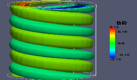
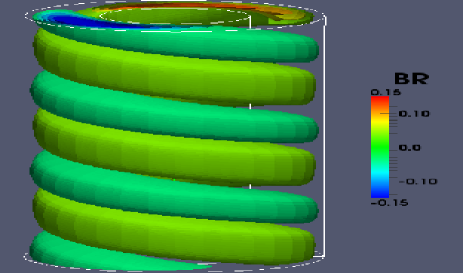
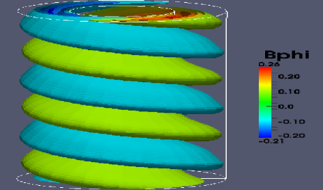
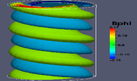
Figure 10: The components (left: radial component, right: azimuthal component) of the magnetic pattern in the AMRI domain (fast rotation) for $\beta=10$. Top: $\rm Re=150,\ \ Ha=50$ ( minimum); bottom: $\rm Re=200,Ha=80$. The fields are normalized with $B_{\rm in}$. $\mu_{B}=1$, $\rm Pm=1$.

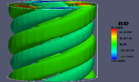
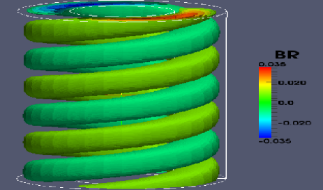
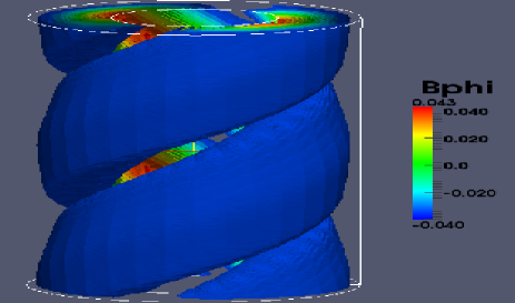
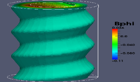
Figure 11: Components of the magnetic pattern (left: radial component, right: azimuthal component) for TI (slow rotation). $\rm Re=30$, $\rm Ha=130$. Top: $\beta=2$, Bottom: $\beta=10$. The fields are normalized with $B_{\rm in}$. $\mu_{B}=1$, $\rm Pm=1$.

Unlike the AMRI, the TI yields right-handed spirals (Fig. 11). The pattern in the bottom row ($\beta=10$) has an azimuthal wavenumber $m=1$, in accordance with the instability map Fig. 8. The top row, however, represents a pattern with $m=2$, which also exists in the nonlinear regime as predicted by the bottom plot of Fig. 8. In this case there is no clear correlation between the radial and azimuthal components of the field perturbations.

The nonlinear simulations, of course, do also provide the amplitudes of the fields in the resulting magnetic pattern. Here we only note the overall result that the AMRI produces much higher field strengths than the TI. One might speculate that the AMRI exists due to the differential rotation which is always able to induce strong fields but a detailed study of the energy aspects of the magnetic instabilities is out of the scope of the present paper.

References

- (1) S. A. Balbus and J. F. Hawley, Astrophys. J. 376, 214 (1991).
- (2) E. P. Velikhov, Sov. Phys. JETP 9, 995 (1959).
- (3) D. Michael, Mathematica 1, 45 (1954).
- (4) R. J. Tayler, Mon. Not. R. Astron. Soc. 161, 365 (1973).
- (5) R. Hollerbach, V. Teeluck and G. Rüdiger, PRL (accepted).
- (6) L. N. Howard and A. S. Gupta, J. Fluid Mech. 14, 463 (1962).
- (7) R. Hollerbach and G. Rüdiger, Phys. Rev. Lett. 95, 124501 (2005).
- (8) G. Rüdiger, R. Hollerbach, F. Stefani, T. Gundrum, G. Gerbeth and R. Rosner, Astrophys. J. 649, L145 (2006).
- (9) F. Stefani, T. Gundrum, G. Gerbeth, G. Rüdiger, M. Schultz, J. Szklarski and R. Hollerbach, Phys. Rev. Lett. 97, 184502 (2006).
- (10) S. Chandrasekhar, Hydrodynamic and Hydromagnetic Stability (Clarendon, Oxford 1961).
- (11) E. Knobloch, Phys. Fluids 8, 1446 (1996).
- (12) G. Rüdiger and R. Hollerbach, Phys. Rev. E 76, 068301 (2007).
- (13) A. Bonanno and U. Urpin, Astron. Astrophys. 488, 1 (2008).
- (14) G. Rüdiger and M. Schultz, Astron. Nachr. 331, 121 (2010).
- (15) M. Gellert, G. Rüdiger and A. Fournier, Astron. Nachr. 328, 1162 (2007).
- (16) A. Fournier, H.-P. Bunge, R. Hollerbach and J.-P. Vilotte, J. Comp. Phys. 204, 462 (2005).