Uniform cross phase modulation for nonclassical radiation pulses

Abstract

We propose a scheme to achieve a uniform cross phase modulation (XPM) for two nonclassical light pulses and study its application for quantum non-demolition measurements of the photon number in a pulse and for controlled phase gates in quantum information. We analyze the scheme by quantizing a common phenomenological model for classical XPM. Our analysis first treats the ideal case of equal cross-phase modulation and pure unitary dynamics. This establishes the groundwork for more complicated studies of non-unitary dynamics and difference in phase shifts between the two pulses where decohering effects severely affect the performance of the scheme.

I Introduction

Optical cross phase modulation (XPM) is a specific variant of nonlinear optical phenomena of Kerr type in which the refractive index $n_{1}$ of light in pulse 1 varies linearly with the intensity $I_{2}$ of another light field, so that $\epsilon_{1}=1+\chi_{1}+\chi_{3}I_{2}$, with $\epsilon_{1}=n_{1}^{2}$ the permittivity of the medium, $\chi_{1}$ the linear, and $\chi_{3}$ the nonlinear XPM susceptibility, respectively. In ordinary optical media this effect is small and requires large intensities, but the proposal by Schmidt and Imamoǧlu Schm96 to generate giant nonlinearities using electromagnetically induced transparency (EIT) Harr97 ; boller91 ; Lukin97 has made very large Kerr coefficients possible Schm96 ; Harr99 ; Hauu99 ; Bajcsy03 ; kang03 and may even lead to nonlinear effects at the single-photon level Luki00 ; Pett02 ; Mats03 ; ottaviani03 ; Pett04 ; rebic04 ; Zeng06 .

XPM is a strong candidate for the design of optical quantum controlled-phase gates (CPG) for photonic quantum information processing Chuu95 ; nemoto05 ; munro05 , in which two single-photon pulses would become entangled. For sufficiently high fidelity, XPM would allow the construction of deterministic gates, as opposed to the non-deterministic optical CPG that are based on linear optics Sana95 and establish entanglement through measurements Knil01 . It has been suggested that double EIT – EIT for both pulses with matched group velocities – would generate the maximal XPM phase shift because matched group velocities for both photons would maximize their interaction time Luki00 ; Pett02 ; Mats03 ; ottaviani03 ; Pett04 ; rebic04 ; Zeng06 . However, XPM based on double EIT still faces some challenges: (i) to achieve sufficiently high intensities at the two-photon level, the photon pulses must be tightly confined in the transversal direction; (ii) if the nonlinear medium has a finite response time, the matter-light interaction unavoidably induces noise. It was shown by Shapiro Shap06 that for a large class of XPM models this would limit the fidelity of a CPG to only about 65%. Further theoretical studies on this topic confirmed these results shapiro:022301 ; shapiro:njp2007 ; koshino:063807 ; leungXPM2008 . (iii) For matched co-propagating pulses, each point of the pulse will experience a different XPM phase shift because the intensity, and hence the refractive index $n_{1}$, varies over the shape of the pulse. This would severely affect the entanglement between the pulses.

In this paper we will address the third problem and do not deal with problem (i) and (ii), i.e., we will assume that transverse confinement of the photon pulses can be achieved by some means, such as hollow core fibers PhysRevLett.75.3253 ; Gehring:JLightwTechn2008 ; hollowFibres ; londero:043602 or nano wires LukinNanoWire , and that the medium’s response time is so short that the polarizability of the medium reacts instantaneously to a photon’s electric field. The omission of the noise associated with a finite response time is also made for clarity because, despite that we are working in the instantaneous regime, we will show that very similar effects may appear if the two light pulses have different group velocities.

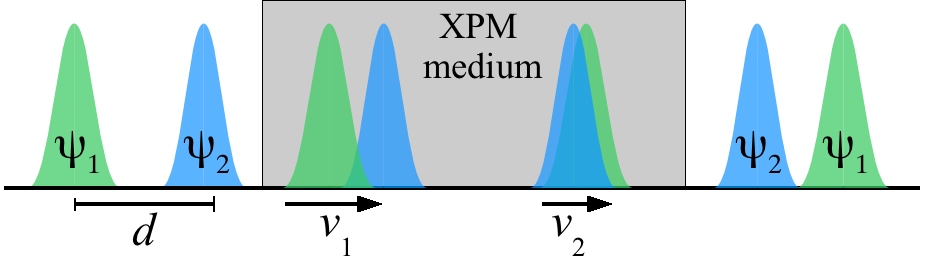
Figure 1: Scheme to achieve uniform XPM: two light pulses $\psi_{1},\psi_{2}$ travel at different group velocities $v_{1}>v_{2}$ through an XPM medium such that $\psi_{1}$ can overtake $\psi_{2}$. $d$ denotes the initial distance between the two pulses.

To solve problem (iii) we extend an idea of Rothenberg Josh93 who demonstrated a uniform XPM phase shift for classical pulses in birefringent fibers: two light pulses travel through a XPM medium with different group velocities $v_{1}>v_{2}$, see Fig. 1. Pulse 2 (blue) reaches the Kerr medium first but pulse 1 (green) is faster and leaves it first. While the pulses overlap they interact via the Kerr effect, which is proportional to the pulse intensity. Because pulse 1 overtakes pulse 2 the acquired phase shift will be averaged over the pulse shape and thus be nearly uniform.

Here we generalize this idea to characterize the propagation of quantized light pulses and show that a uniform phase shift can also be achieved for quantum interference effects. We will show that quantizing the classical XPM equations is generally a subtle problem which may make the introduction of noise terms similar to those in problem (i) necessary. We exploit our results to suggest experiments for quantum non-demolition (QND) measurement of photon numbers and CPG.

This paper is organized as follows. In Sec. II we will present a phenomenological quantum model for XPM between two pulses with different group velocities and discuss the two cases of unitary and non-unitary dynamics in this model. In Sec. III we present proposals for QND measurement of photon numbers and CPG and show that they can have a high fidelity in this case. The analysis of these proposals for the non-unitary case is presented in Sec. IV. Several appendices contain details of our derivation.

II Pulse propagation with mismatched group velocities

We consider two quantized light pulses that travel through an XPM medium with different group velocities $v_{1}>v_{2}$. We assume that the light pulses are transversally confined so that we can restrict the model to one spatial dimension. In classical fiber optics this situation is commonly described by the set of equations agrawal06 ; PTL6-733 ; JRLR29-57

$$\left(\frac{1}{v_{i}}\partial_{t}+\partial_{z}\right){\cal E}_{i}(z,t) =-{\rm i}\gamma_{i}(I_{i}(z,t)+2I_{3-i}(z,t)){\cal E}_{i}(z,t),$$ (1)

with imaginary unit ${\rm i}=\sqrt{-1}$. Here ${\cal E}_{i}$ is the field amplitude of pulse $i=1,2$, $I_{i}=|{\cal E}_{i}|^{2}$ is proportional to the intensity, and $\gamma_{i}$ is the self phase modulation (SPM) coefficient. The XPM coefficient is given by $2\gamma_{i}$. This model is local and instantaneous; i.e., the light field ${\cal E}_{1}(z,t)$ is only affected by ${\cal E}_{2}(z,t)$ and vice versa.

In the context of SPM, Joneckis and Shapiro have shown that in a local and instantaneous quantum model, where ${\cal E}_{i}$ represents a field operator, infinite zero-point fluctuations do occur shapiro:josab1993 . They suggested taking a finite response time of the medium into account to avoid singularities. We instead propose a model in which the medium’s response is still instantaneous but spatially nonlocal, i.e., ${\cal E}_{1}(z,t)$ can be affected by ${\cal E}_{2}(z^{\prime},t)$. The most general macroscopic model that describes such an instantaneous interaction between two light pulses of different group velocities is then given by

$$\left(\frac{1}{v_{i}}\partial_{t}+\partial_{z}\right){\cal E}_{i}(z,t) =-{\rm i}\int_{-\infty}^{\infty}dz^{\prime}I_{3-i}(z^{\prime},t)$$

$$\times V_{i}(z-z^{\prime}){\cal E}_{i}(z,t).$$ (2)

Here and henceforth ${\cal E}_{i}$ denotes the field operator and $I_{i}(z,t)={\cal E}_{i}^{\dagger}(z^{\prime},t){\cal E}_{i}(z^{\prime},t)$ the intensity operator. The quantities $V_{i}(z-z^{\prime})$ are spatially nonlocal interaction potentials between the two pulses generated by the atomic medium. To avoid causality violation its support must be much smaller than the wavelength of light. We will assume that $V_{i}(z-z^{\prime})$ is essentially zero if the distance between $z$ and $z^{\prime}$ is much larger than the Bohr radius. One can consider the introduction of nonlocal potentials as a regularization of the classical theory (1) by smearing out the point interaction. In the limit of sharp potentials, $V_{i}(z)={\cal V}_{i}\delta(z)$, the regularized model reduces to Eq. (1) for XPM coefficient $\gamma_{i}={\cal V}_{i}/2$.

Multi-photon pulse dynamics should account for SPM, but we omit this effect here in order to focus on XPM. When XPM is placed in the context of interferometry, which gives phase an operational meaning, pairs of nonlinear media in both paths can offset SPM Sanders:JOSAB92 . Alternatively SPM is not present for single-photon pulses because a single photon cannot induce SPM on itself.

The multi-mode field operators $\mathcal{E}_{i}(z)$ satisfy the commutation relations

$$[{\cal E}_{i}(z,t),{\cal E}_{j}^{\dagger}(z^{\prime},t)] =\frac{\hbar\omega_{i}}{2\epsilon_{0}A}\delta_{ij}\delta(z-z^{\prime})\equiv\eta\delta_{ij}\delta(z-z^{\prime}),$$ (3)

with $\omega_{i}$ the central frequency of pulse $i$ and $A$ the transverse area of the pulses. The field is assumed to be in a single mode with the $i^{\rm th}$ longitudinal mode function given by $\psi_{i}(z)$. Photons in this mode are annihilated by the operator

$$a_{i}[u] =\frac{1}{\sqrt{\eta}}\int_{-\infty}^{\infty}dz\,\psi^{*}_{i}(z-u)\,\hat{\cal{E}}_{i}(z,0)\;,$$ (4)

For later use we have included a possible shift $u$ of the wavefunction. If the shift is zero we will sometimes suppress this notation and write $a_{i}\equiv a_{i}[0]$.

If Eq. (2) is taken to be the dynamical equation of the quantum fields ${\cal E}_{i}$ one has to be careful with its interpretation. It can be shown that Eq. (2) can be expressed as $\partial_{t}{\cal E}_{i}=-{\rm i}[{\cal E}_{i},H]$ for some Hamiltonian $H$ if and only if $v_{1}V_{1}(z)=v_{2}V_{2}(z)$. In other words, a unitary evolution of the quantum fields will only occur if the two interaction potentials are proportional to each other, with the proportionality factor given by the ratio of the group velocities. In absence of absorption or other decohering processes one therefore would assume that in the quantum model this relation must be fulfilled. However, in the corresponding classical models for XPM pulse propagation this is generally not the case agrawal06 ; PTL6-733 ; JRLR29-57 .

In our subsequent analysis we will therefore first assume that the evolution is unitary and analyze our proposals within this framework. In Sec. IV we then will develop a consistent phenomenological quantum model for non-unitary evolution using techniques of open quantum systems and reassess the proposals for this case footnote1 .

III XPM for unitary evolution

To devise a scheme for CPG and QND measurements of the photon number we will assume that the dynamics is unitary; in this case the interaction potentials can generally be written as $V_{i}(z)=V(z)/v_{i}$, with $V(z)$ a Hamiltonian interaction potential. However, we will make use of this relation only after deriving general results in order to facilitate the extension to non-unitary dynamics.

The solution of Eq. (2) for the propagation of light in an infinitely extended XPM medium is

$${\cal E}_{i}(z,t) =U_{3-i}(z,t){\cal E}_{i}(z-v_{i}t,0),$$ (5)

$$U_{i}(z,t) =\exp\Bigg{(}-{\rm i}\int_{-\infty}^{\infty}\hat{I}_{i}(z^{\prime},0)\frac{v_{3-i}}{v_{i}-v_{3-i}}$$

$$\hskip 14.22636pt\times\theta_{3-i}\left(z-z^{\prime}-v_{3-i}t\,,\,[v_{i}-v_{3-i}]t\right)dz^{\prime}\Bigg{)},$$ (6)

$$\theta_{i}(z_{1},z_{2}) \equiv\int_{0}^{z_{2}}dz^{\prime}\,V_{i}(z_{1}-z^{\prime})\;.$$ (7)

The function $\theta_{i}(z_{1},z_{2})$ will play a central role in determining the Kerr phase shift. One important property is that for a symmetric potential, $V_{i}(-z)=V_{i}(z)$, we have $\theta_{i}(-z_{1},-z_{2})=-\theta_{i}(z_{1},z_{2})$.

III.1 Quantum non-demolition measurement of photon numbers

As a first application we consider a QND measurement of the number of photons San89 in mode 2. This can be accomplished by sending a strong classical pulse in mode 1, which can be described by a coherent state $|\alpha\rangle$, together with an $n$ photon pulse $|n\rangle$ in mode 2 through the XPM medium. Single-mode treatments predict that in this case the phase of the classical pulse will be shifted by an amount that is proportional to $n$. Here we show that the uniform cross phase shift that we suggest will accomplish precisely this.

The initial state of the two light pulses before they start to interact takes the form $|\psi\rangle=|\alpha\rangle\otimes|n\rangle$ where the two kets refer to mode 1 and 2, repectively. Using the shift operator $D_{1}(\alpha)=\exp(\alpha a_{1}^{\dagger}-\alpha^{*}a_{1})$ this can be expressed as

$$|\psi\rangle=\frac{1}{\sqrt{n!}}D_{1}(\alpha)(a_{2}^{\dagger})^{n}|0\rangle.$$ (8)

The complex amplitude of the classical pulse at time $t$ and position $z$ is given by $\langle\psi|{\cal E}_{1}(z,t)|\psi\rangle$. Its phase can be measured using homodyne detection tyc:JPA2004 , for instance, which more specifically measures the observable $X(\vartheta)=e^{{\rm i}\vartheta}{\cal E}_{1}(z,t)+e^{-{\rm i}\vartheta}{\cal E}_{1}^{\dagger}(z,t)$. Using Eq. (45) it is easy to see that

$$D_{1}^{\dagger}(\alpha){\cal E}_{1}(z,0)D_{1}(\alpha)={\cal E}_{1}(z,0)+\alpha\sqrt{\eta}\psi_{1}(z)\;.$$ (9)

Exploiting this and solution (5) we get

$$\langle\psi|{\cal E}_{1}(z,t)|\psi\rangle =\frac{\alpha\sqrt{\eta}}{n!}\psi_{1}(z-v_{1}t)\langle 0|a_{2}^{n}U_{2}(z,t)(a_{2}^{\dagger})^{n}|0\rangle$$

$$=\frac{\alpha\sqrt{\eta}}{n!}\psi_{1}(z-v_{1}t)\langle 0|a_{2}^{n}(\tilde{a}_{2}^{\dagger}[0;z,t])^{n}|0\rangle,$$ (10)

where we have used Eq. (46) and introduced an XPM-modified annihilation operator

$$\tilde{a}_{i}[u;z,t] \equiv\frac{1}{\sqrt{\eta}}\int_{-\infty}^{\infty}dz^{\prime}\,\psi^{*}_{i}(z^{\prime}-u)\,\hat{\cal{E}}_{i}(z^{\prime},0)$$

$$\times e^{-{\rm i}\eta\frac{v_{3-i}}{v_{i}-v_{3-i}}\theta_{3-i}(z-z^{\prime}-v_{3-i}t,(v_{i}-v_{3-i})t)}\;.$$ (11)

The physical interpretation of Eq. (11) is that the wavepacket $\psi^{*}_{i}(z^{\prime}-u)$ is multiplied by a spatially varying phase factor that is given by the exponential in Eq. (11) and incorporates the effect of XPM on the light pulses.

The expectation value for field 2 in Eq. (10) can then be reduced to

$$\langle 0|a_{2}^{n}(\tilde{a}_{2}^{\dagger}[0;z,t])^{n}|0\rangle =n![a_{2},\tilde{a}_{2}^{\dagger}[0;z,t]\,]^{n},$$ (12)

so that

$$\langle{\cal E}_{1}(z,t)\rangle =\alpha\sqrt{\eta}\psi_{1}(z-v_{1}t)$$

$$\times\bigg{(}\int dz^{\prime}\,|\psi_{2}(z^{\prime})|^{2}e^{{\rm i}\eta\frac{v_{1}}{\Delta v}\theta_{1}(z^{\prime}-z+v_{1}t,\Delta v\,t)}\bigg{)}^{n},$$ (13)

with $\Delta v\equiv v_{1}-v_{2}$.

To better understand the physical implications of Eq. (13) we consider the specific configuration depicted in Fig. 1. The classical mode $\psi_{1}$ is initially centered around the origin while the $n$-photon pulse in mode $\psi_{2}$ is a distance $d$ to the right of it footnote2 . Both pulses are moving to the right, but pulse 1 is faster. The first line in Eq. (13) is basically the amplitude of the classical pulse $\psi_{1}$ at time $t$ in absence of the XPM medium. The pulse is centered around $z=v_{1}t$. Hence, to achieve an maximum phase contrast, we should observe the field at this point. The exponential in Eq. (13) is then proportional to $\theta_{1}(z^{\prime},\Delta v\,t)$.

In Appendix B it is shown that for any potential $V_{i}(z)$ that is consistent with causality, the function $\theta_{1}(z^{\prime},\Delta v\,t)$ is nearly constant between the lines $\Delta v\,t=z^{\prime}$ and $z^{\prime}=0$ and zero outside of this range. The support of the initial wavepacket $\psi_{2}(z^{\prime})$ is in the area $z^{\prime}>0$ and peaked around $z^{\prime}=d$. For sufficiently large times, such that $\Delta v\,t\gg d$, the support of $\psi_{2}(z^{\prime})$ is therefore completely inside the domain where $\theta_{1}(z^{\prime},\Delta vt)\approx{\cal V}_{1}$, with the constant

$${\cal V}_{i}\equiv\int_{-\infty}^{\infty}dz\,V_{i}(z).$$ (14)

This condition corresponds to the requirement that the classical pulse 1 had enough time to overtake the $n$-photon pulse 2. Because the mode function $\psi_{2}$ is normalized we thus find

$$\langle{\cal E}_{1}(v_{1}t,t)\rangle =\alpha\sqrt{\eta}\,\psi_{1}(0)e^{-{\rm i}n\phi_{1}},$$ (15)

$$\phi_{i} \equiv\frac{\eta v_{i}{\cal V}_{i}}{\Delta v}\;.$$ (16)

We remark that $\phi_{1}=\phi_{2}$ for unitary dynamics. Eq. (15) is precisely the result that one would obtain in a single-mode treatment. Hence, for unitary dynamics a mismatch in the group velocities of two pulses that allows one pulse to overtake the other in a Kerr medium will result in a uniform phase shift for QND measurements of the photon number. In practice, overtaking will impose a minimum requirement on the length of the Kerr medium and SPM will lead to a distortion of the signal.

III.2 Controlled-Phase Gate

Our proposal to build a CPG extends previous designs to build quantum gates using XPM Chuu95 ; rebic06 by ensuring a uniform XPM phase shift. In a controlled phase gate, two qubits with logical basis states $|0\rangle,|1\rangle$ are manipulated in such a way that the state acquires a phase shift $\beta$ only if both qubits are in the logical state $|1\rangle\otimes|0\rangle$. In other words, a CPG is a unitary operator that maps the basis states $|kl\rangle\equiv|k\rangle\otimes|l\rangle$ to footnote3

$$U_{\text{CPG}}|kl\rangle=e^{{\rm i}\,k(1-l)\,\beta}|kl\rangle\;,\;k,l=0,1\;.$$ (17)

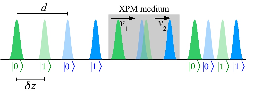
Figure 2: Construction of a controlled phase gate for two time-bin qubits using uniform XPM.

With the uniform cross phase shifter discussed above, such a gate can be implemented for time-bin encoded photonic qubits as indicated in Fig. 2. In this case each optical field ${\cal E}_{n}$ carries one photon. For each photon the logical basis states are encoded in two wavepackets, one of which is delayed compared to the other. The logical state $|0\rangle$ for qubit $n$ ($n=1,2$) can be encoded in wavepackets $\psi_{n}(z)$ so that photons in this state are annihilated by operator $a_{n}=a_{n}[0]$. The logical state $|1\rangle$ can be encoded in wavepackets that are shifted to the right, $\psi_{n}(z-\delta z)$; photons in this state are annihilated by the operators $a_{n}[\delta z]$. A CPG can then be constructed by arranging the initial distances between the wavepackets in such a way that the only states that do overlap inside the XPM medium are state $|1\rangle$ of the first qubit and state $|0\rangle$ of the second qubit. For all other logical states the wavepackets in the two field modes never overlap so that there is no XPM effect.

The logical basis states for two time-bin encoded qubits at time $t$ are given by the set

$$|ij(t)\rangle=a_{1}^{\dagger}[\delta z^{(1)}_{i}+v_{1}t]\,a_{2}^{\dagger}[\delta z^{(2)}_{j}+v_{2}t]\,|0\rangle,$$ (18)

for $(\delta z^{(1)}_{i},\delta z^{(2)}_{j})=(0,0),(0,\delta z),(\delta z,0),(\delta z,\delta z)$ for $(i,j)=(0,0),(0,1),(1,0),(1,1)$, respectively. The factors $v_{i}t$ represent an explicit time dependence in the definition of the logical states such that they are co-moving with the wavepackets at group velocity $v_{i}$.

We consider the case that the two photons are initially prepared in a pure two-qubit state $|\psi(0)\rangle=\sum_{kl}c_{kl}|kl(0)\rangle$. To characterize the performance of the CPG we need to obtain the logical components $\rho_{ij;kl}(t)=\langle ij(t)|\rho(t)|kl(t)\rangle$ of the density matrix $\rho(t)$ at time $t$. A somewhat tedious calculation that can be found in App. C.1 leads to

$$\rho_{ij;kl}(t) =X_{kl}^{*}X_{ij},$$ (19)

with

$$X_{ij} =c_{ij}\int dz_{1}\,dz_{2}\,|\psi_{1}(z_{1})\,\psi_{2}(z_{2}+d)|^{2}$$

$$\times e^{-{\rm i}\eta\frac{v_{2}}{\Delta v}\theta_{2}(z_{2}-z_{1}+d+\delta z^{(2)}_{j}-\delta z^{(1)}_{i},\Delta vt)}.$$ (20)

The phase factor in Eq. (20) determines the XPM effect. We now prove that it is only nontrivial for the logical state $|10\rangle$ because only in this case the associated wavepackets overtake each other.

The phase factor is proportional to the function $\theta_{2}(z_{2}-z_{1}+d+\delta z^{(2)}_{j}-\delta z^{(1)}_{i},\Delta vt)$ which, according to Appendix B, is nearly constant for a given range of its two variables. Ignoring the variables $z_{i}$ for the moment we consider $\theta_{2}(d+\delta z^{(2)}_{j}-\delta z^{(1)}_{i},\Delta vt)$ instead. For the four states $00,01,10,11$ the first argument takes the values $d,d+\delta z,d-\delta z$, and $d$ respectively. If we choose the time $t$ for which the photons are interacting such that $d-\delta z<\Delta vt<d,d+\delta z$ then $\theta_{2}=0$ for $ij=00,01,11$ and $\theta_{2}={\cal V}_{2}$ for $ij=10$. Hence only the latter combination will experience an XPM phase shift. This conclusion also holds if we re-introduce the variables $z_{i}$ because they only vary over the support of the two wavepackets, which is smaller than $d,\delta z$; the value of $\theta_{2}$ therefore does not change. Thus we arrive at

$$X_{ij} =c_{ij}e^{-{\rm i}i(1-j)\phi_{2}},$$ (21)

and the density matrix elements become

$$\rho_{ij;kl}(t) =c_{ij}c_{kl}^{*}e^{-{\rm i}(i(1-j)-k(1-l))\phi_{2}}.$$ (22)

Let us now work out the performance of the CPG by calculating the concurrence PhysRevLett.80.2245 of the density matrix (22) for a specific initial product state $|\psi(0)\rangle=(|0\rangle+|1\rangle)\otimes(|0\rangle+|1\rangle)/2$, which corresponds to $c_{ij}=\frac{1}{2}$ for all $i,j$. The concurrence $C$ of the density matrix (22) then evaluates to $C=|\sin(\phi_{2}/2)|$. This indicates a perfect CPG because the initial product state is transformed into a maximally entangled state provided one can achieve a large phase shift $\phi_{2}=\pi$.

IV XPM with Non-Hamiltonian coupling

In the previous section we have devised a scheme to create uniform XPM for quantized light pulses for the special case of unitary dynamics for which $v_{1}V_{1}(z)=v_{2}V_{2}(z)$. The theory behind this scheme corresponds to a regularized quantization of the classical theory (1) for the case that the XPM coefficients are related by $v_{1}\gamma_{1}=v_{2}\gamma_{2}$. However, in classical optics this relation between the two XPM coefficients is not generally adopted. In this section we therefore study the quantization of the classical model with $v_{1}\gamma_{1}\neq v_{2}\gamma_{2}$ and its implications for quantum information processing. Because the model needs to be regularized, we consider the general case with two non-local interaction potentials that fulfill $v_{1}V_{1}(z)\neq v_{2}V_{2}(z)$.

The discussion in Sec. II has revealed that the quantum dynamics in this case must be non-unitary because there is no Hamiltonian that can generate the equations of motion. As Eq. (2) is based on a phenomenological model that does not explicitly include absorption or dissipation, the origin for this non-unitarity cannot be identified in an unambiguous way. There might be implicit absorption processes hidden in the model, although we strongly doubt that this is the case because the dynamics does not have a structure that is comparable to the Lindblad form lindblad76 . Another possibility is that the external fields that usually are needed for EIT-based XPM media may induce energy fluctuations that lead to non-Hamiltonian dynamics. Yet another possibility is that the direct quantization of the classical theory (1) ignores the averaging processes that are associated with a macroscopic decription of electrodynamics jackson99 . Such averaging procedures lead to loss of information, which may induce decoherence in a quantum system.

Despite this ambiguity with respect to the cause of non-unitary dynamics it is worthwhile studying this situation because one can gain a better understanding of the quantization of a new class of classical models. Furthermore, even if the theory that we develop below cannot include the microscopic details behind the XPM interaction it nevertheless should help to estimate the effects of a mismatch between the XPM coefficients.

In the case $v_{1}V_{1}(z)\neq v_{2}V_{2}(z)$, Eq. (5) still provides an exact solution to the dynamical equation of motion. However, this solution is inconsistent with basic requirements of quantum field theory. To illustrate this point we consider the equal-time commutation relations between the Heisenberg field operators, which should agree with the commutation relations between the respective Schrödinger operators. In our case this principle is violated because

$${\cal E}_{2}(z^{\prime},t){\cal E}_{1}(z,t) ={\cal E}_{1}(z,t){\cal E}_{2}(z^{\prime},t)e^{-{\rm i}\Phi(z^{\prime}-z,t)},$$ (23)

$$\Phi(z^{\prime}-z,t) \equiv\frac{\eta}{\Delta v}\big{(}v_{1}\theta_{1}(z^{\prime}-z+\Delta vt,\Delta vt)$$

$$\hskip 19.91692pt-v_{2}\theta_{2}(z^{\prime}-z+\Delta vt,\Delta vt)\big{)},$$ (24)

despite $[{\cal E}_{1}(z,0),{\cal E}_{2}(z^{\prime},0)]=0$.

The conventional way to deal with non-Hamiltonian dynamics in the Heisenberg picture is to introduce Langevin noise operators. In the context of nonlinear optics this has first been done by Boivin et al. haus94 in the case of time-dependent self-phase modulation.

We now show that a similar approach can also be made for instantaneous XPM between two light pulses with different group velocities. Following Ref. haus94 we introduce Hermitian decoherence operators $m_{i}(z,t)$ such that the dynamical equations are modified to

$$\left(\frac{1}{v_{i}}\partial_{t}+\partial_{z}\right){\cal E}_{i}(z,t) =-{\rm i}\Big{(}\int_{-\infty}^{\infty}dz^{\prime}I_{3-i}(z^{\prime},t)$$ (25)

$$\times V_{i}(z-z^{\prime})+m_{i}(z,t)\Big{)}{\cal E}_{i}(z,t)\;.$$

The decoherence operators commute with all field operators. We adopt the frequently used assumption of $\delta$-correlated decoherence,

$$[m_{i}(z,t)\,,\,m_{j}(z^{\prime},t^{\prime})]={\rm i}\eta\left(\textstyle{\frac{V_{i}(z-z^{\prime})}{v_{j}}-\frac{V_{j}(z-z^{\prime})}{v_{i}}}\right)\delta(t-t^{\prime}).$$ (26)

The solution of Eq. (25) can be written as

$${\cal E}_{i}(z,t) =R_{i}(z,t)\,U_{3-i}(z,t)\,{\cal E}_{i}(z-v_{i}t,0),$$ (27)

$$R_{i}(z,t) =\exp\left(-{\rm i}v_{i}\int_{0}^{t}dt^{\prime}\,m_{i}(z-v_{i}(t-t^{\prime}),t^{\prime})\right)\;.$$ (28)

Using the commutation relations (26) it is not hard to show that

$$R_{1}^{\dagger}(z,t)\,R_{2}(z^{\prime},t)\,R_{1}(z,t) =R_{2}(z^{\prime},t)\,e^{{\rm i}\Phi(z^{\prime}-z,t)},$$

$$R_{2}^{\dagger}(z,t)\,R_{1}(z^{\prime},t)\,R_{2}(z,t) =R_{1}(z^{\prime},t)\,e^{-{\rm i}\Phi(z-z^{\prime},t)}\;.$$ (29)

As a consequence, solution (27) fulfills the equal-time commutation relations. Introducing the decoherence term in Eq. (25) has thus led to a consistent quantum field theory of XPM for light pulses with different group velocities.

IV.1 Controlled-Phase Gate

To characterize the performance of a CPG in the case of non-unitary dynamics we can repeat the steps discussed in Sec. III.2 with solution (5) replaced by Eq. (27). Finding the logical density matrix elements must then be done within an open system approach that is described in App. C.2. As a result, the factors $X_{ij}$ become operators on the Hilbert space of the environment (on which the decoherence operators act) and Eq. (21) is replaced by

$$X_{ij} =c_{ij}e^{-{\rm i}i(1-j)\phi_{2}}\int dz_{1}\,dz_{2}\,|\psi_{1}(z_{1})\,\psi_{2}(z_{2}+d)|^{2}$$

$$\times R_{1}(z_{1}+v_{1}t+\delta z^{(1)}_{i},t)R_{2}(z_{2}+d+v_{2}t+\delta z^{(2)}_{j},t).$$ (30)

The logical density matrix elements take the form

$$\rho_{ij;kl}(t) =\text{Tr}_{\text{E}}\big{(}\rho_{\text{E}}(0)X_{kl}^{\dagger}X_{ij}\big{)},$$ (31)

with $\text{Tr}_{\text{E}}$ indicating the trace over the environment degrees of freedom and $\rho_{\text{E}}(0)$ the initial state of the environment.

To keep the discussion concise we assume that the photon pulses are very sharp. We then can replace the squares of the wavefunctions by $\delta$ distributions and get

$$X_{ij} =c_{ij}e^{-{\rm i}i(1-j)\phi_{2}}R_{1}(v_{1}t+\delta z^{(1)}_{i},t)R_{2}(d+v_{2}t+\delta z^{(2)}_{j},t).$$ (32)

The density matrix elements then become

$$\rho_{ij;kl}(t) =c_{ij}c_{kl}^{*}e^{-{\rm i}(i(1-j)-k(1-l))\phi_{2}}N_{ij;kl}(t),$$ (33)

with the Hermitian decoherence matrix

$$N_{ij;kl}(t) \equiv\Big{\langle}R_{2}^{\dagger}(d+v_{2}t+\delta z^{(2)}_{l},t)R_{1}^{\dagger}(v_{1}t+\delta z^{(1)}_{k},t)$$

$$\times R_{1}(v_{1}t+\delta z^{(1)}_{i},t)R_{2}(d+v_{2}t+\delta z^{(2)}_{j},t)\Big{\rangle}.$$ (34)

In App. C.3) we show that it can be written as

$$N =\left(\begin{array}[]{cccc}1&c_{2}&c_{1}e^{{\rm i}(\phi_{1}-\phi_{2})}&N_{00;11}\\ c_{2}^{*}&1&N_{01;10}&c_{1}\\ c_{1}^{*}e^{-{\rm i}(\phi_{1}-\phi_{2})}&N_{01;10}^{*}&1&c_{2}\\ N_{00;11}^{*}&c_{1}^{*}&c_{2}^{*}&1\end{array}\right),$$ (39)

$$c_{n} \equiv\Big{\langle}R_{n}^{\dagger}(v_{n}t+\delta z,t)R_{1}(v_{n}t,t)\Big{\rangle}.$$ (40)

Hence the influence of decoherence in our model can be described by four complex parameters $N_{00;11}$, $N_{01;10}$, and $c_{n}$. This is a consequence of the approximation of very short pulses. For extended pulses additional decoherence contributions are anticipated.

We again calculate the concurrence of density matrix (33) for the initial product state $c_{ij}=\frac{1}{2}$ for all $i,j$. The specific values of the parameters $N_{00;11}$, $N_{01;10}$, and $c_{n}$ depend on the detailed decoherence model that one employs so that the predictions may vary substantially depending on the assumptions behind the model. We present one particular decoherence model in Appendix D. However, all decoherence models must be consistent with all eigenvalues of the density matrix (22) taking values between 0 and 1.

To simplify the discussion we consider the special case $\phi_{2}=\pi$ for the oft-used assumption that the two interaction potentials $V_{i}(z)$ are equal and independent of the group velocities PTL6-733 ; JRLR29-57 so that ${\cal V}_{1}={\cal V}_{2}$. The phase factor that appears in the decoherence matrix (39) is then $\phi_{1}-\phi_{2}=\pi\Delta v/v_{2}>0$. For a given value of $\phi_{1}-\phi_{2}$ we can derive a “minimal decoherence model” by finding those values of the parameters $N_{00;11}$, $N_{01;10}$, and $c_{n}$ which maximize the concurrence $C$ for a consistent density matrix. Fig. 3 shows the concurrence for this minimal decoherence model as a function of $\phi_{1}-\phi_{2}$. The dots are found through a random search for the parameters $N_{00;11}$, $N_{01;10}$, and $c_{n}$ of the minimal decoherence model. Each dot is based on a sample of typically $10^{7}$ random events. The error in each value is estimated to be about 5%. The concurrence decreases with $\phi_{1}-\phi_{2}$ and becomes zero for $\phi_{1}-\phi_{2}=\pi$. In this case decoherence completely destroys the entangling capacity of the XPM interaction. The numerically determined density matrix then corresponds to a nearly equal mixture of two highly entangled states.

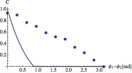
Figure 3: Concurrence as a function of the XPM phase shift for minimal decoherence (dots) and the decoherence model presented in Appendix D (solid line).

Realistic decoherence models would typically predict a less than optimal performance. For instance, the blue line in Fig. 3 shows $C$ for the decoherence model of App. D under the fairly optimistic assumption $\Delta vt=4\sqrt{\pi}w$, where $w$ is the width of a Gaussian potential $V_{1}(z)=V_{2}(z)=V(0)\exp(-z^{2}/w^{2})$. For more realistic values $\Delta vt\gg w$ footnote4 the concurrence would be non-zero only in a very narrow range around $\phi_{1}=\phi_{2}$.

Our phenomenological model therefore suggests that a CPG may not be achievable with XPM unless $\phi_{1}$ is very close to $\phi_{2}$. In most proposals for XPM based on double EIT this could be achieved by a suitable preparation of the atomic gas, although it may require fine tuning of parameters like magnetic fields or pump field intensities. A better way to achieve $\phi_{1}=\phi_{2}$ would be to find a system in which this is guaranteed through microscopic symmetries.

IV.2 Quantum non-demolition measurement of photon numbers

The scheme for a QND measurement of the photon number discussed in Sec. III.1 can easily be extended to the non-unitary case by calculating the measurement signal $\langle{\cal E}_{1}(z,t)\rangle$ using solution (27) instead of (5). The only change is that the measurement result (15) is multiplied by $\langle R_{1}(z,t)\rangle$. This factor depends strongly on the specific decoherence model but generally will lead to a decrease in the contrast of the phase measurement.

To give a rough estimate we consider the decoherence model of App. D in which the noise is generated by an environment consisting of a harmonic oscillator field with a flat frequency distribution. We then have

$$\langle R_{i}(z,t)\rangle=\exp\left(-\frac{\eta}{4}\frac{v_{i}}{v_{3-i}}\Delta v\,t\,V(0)\right).$$ (41)

The decoherence amplitude $\langle R_{i}(z,t)\rangle$ can vary between the optimal value 1, if the interaction potential $V(z)=V_{1}(z)=V_{2}(z)$ vanishes at the origin, and very small values for a sharply peaked potential. We remark that this result also demonstrates the necessity of a non-local potential to avoid the diverging quantum fluctuations in the case $V(z)\propto\delta(z)$ shapiro:josab1993 .

It is instructive to evaluate this for a Gaussian potential $V(z)=V(0)\exp(-z^{2}/w^{2})$ where $V(0)>0$ and the width $w$ should be not substantially larger than an atom. We then find $\phi_{1}-\phi_{2}\approx\sqrt{\pi}V(0)w/\eta$ so that

$$\langle R_{i}(z,t)\rangle\approx\exp\left(-\frac{\phi_{1}-\phi_{2}}{4\sqrt{\pi}}\frac{v_{i}}{v_{3-i}}\frac{\Delta v\,t}{w}\right).$$ (42)

The first factor is proportional to the XPM phase shift difference. The last factor $\Delta v\,t/w$ is typically much larger than one because the length $\Delta v\,t$ must be larger than the width of the light pulses ($t$ is the time needed for one pulse to overtake the other). Hence, for very short (femtosecond) pulses the exponential may be of the same size as the XPM phase shift. Typically, however, it will be much larger. We therefore conjecture that for the QND measurement to be successful the XPM phase shifts $\phi_{i}$ in the two light pulses must also be nearly equal.

V Conclusion

In this paper we have devised a scheme to generate a uniform XPM for quantum information processing and applied it to characterize the fidelity of a QND measurement of the number of photons in a light pulse and the performance of a deterministic CPG. The analysis is based on a regularized quantization (2) of a common phenomenological model for the classical XPM effect between two light pulses with different group velocities.

When the pulses overtake each other while traveling through a nonlinear medium the induced XPM phase shift $\phi_{i},i=1,2,$ is uniform over each pulse. For $\phi_{1}=\phi_{2}$ the dynamics is unitary and predicts perfect fidelities for QND measurement and CPG. For $\phi_{1}\neq\phi_{2}$ a decoherence effect must be introduced to keep the model consistent, and this decoherence significantly affects the fidelity of the gate and the QND measurement.

Appendix A Useful commutation relations

In this appendix we will summarize a number of commutation relations that will be useful in deriving our main results.

The effect of XPM on the pulse propagation is governed by the action of the unitary operators $U_{i}=U_{i}(z,t)$ of Eq. (6) on the field operators,

$$U_{i}^{\dagger}{\cal E}_{i}(z^{\prime},0)U_{i} ={\cal E}_{i}(z^{\prime},0)\exp\Big{(}-{\rm i}\eta\frac{v_{3-i}}{v_{i}-v_{3-i}}$$

$$\times\theta_{3-i}(z-z^{\prime}-v_{3-i}t,(v_{i}-v_{3-i})t)\Big{)},$$ (43)

$$U_{i}{\cal E}_{i}(z^{\prime},0)U_{i}^{\dagger} ={\cal E}_{i}(z^{\prime},0)\exp\Big{(}{\rm i}\eta\frac{v_{3-i}}{v_{i}-v_{3-i}}$$

$$\times\theta_{3-i}(z-z^{\prime}-v_{3-i}t,(v_{i}-v_{3-i})t)\Big{)}.$$ (44)

The effect of XPM on the annihilation operator for photons in mode $i$ can be derived from the commutation relations

$$[a_{i}[u],\mathcal{E}_{i}^{\dagger}(z,0)] =\sqrt{\eta}\psi_{i}^{*}(z-u),$$ (45)

and

$$U_{i}^{\dagger}(z,t)\,a_{i}[u]U_{i}(z,t)=\tilde{a}_{i}[u;z,t],$$ (46)

with $\tilde{a}_{i}[u;z,t]$ of Eq. (11).

Appendix B Simplification of the phase shift

If the potential $V_{i}(z)$ has a finite range $r$, so that it vanishes for $|z|>r$, then $\theta_{i}(z_{1},z_{2})$ has generally a shape similar to Fig. 4.

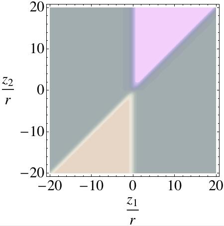
Figure 4: The function $\theta_{i}(z_{1},z_{2})$ for a Gaussian potential $V_{i}(z)$ of width $r$.

It is essentially zero outside the “edges” depicted in the figure and has an extended plateau between the lines $z_{1}=0$ and $z_{1}=z_{2}$. The value on the plateau is given by $\text{sign}(z_{2}){\cal V}_{i}$, with ${\cal V}_{i}$ defined in Eq. (14). The only region where $\theta_{i}(z_{1},z_{2})$ varies significantly are bands of width $2r$ around the lines $z_{1}=0$ and $z_{1}=z_{2}$, and only this transition region depends on the details of the potential. If the range $r$ is much smaller than the optical wavelength we can ignore the transition region so that $\theta_{i}(z_{1},z_{2})$ can be replaced by the plateau value between the lines,

$$\theta_{i}(z_{1},z_{2})\approx\left(\theta(z_{1})\,\theta(z_{2}-z_{1})-\theta(-z_{1})\,\theta(z_{1}-z_{2})\right){\cal V}_{i}\;,$$ (47)

with $\theta(z)$ the step function.

Appendix C Derivation of the action of a CPG on the density matrix

C.1 Unitary dynamics

The evolution of the density matrix $\rho$ can be expressed with the aid of a unitary operator $U(t)$ such that $\rho(t)=U(t)\rho(0)U^{\dagger}(t)$, with

$$\rho(0)=\sum_{i^{\prime},j^{\prime},k,^{\prime}l^{\prime}}c_{k^{\prime}l^{\prime}}^{*}c_{i^{\prime}j^{\prime}}|i^{\prime}j^{\prime}(0)\rangle\langle k^{\prime}l^{\prime}(0)|.$$ (48)

The logical matrix elements of the density matrix can then be expressed as $\rho_{ij;kl}(t)=\langle ij(t)|U(t)\rho(0)U^{\dagger}(t)|kl(t)\rangle$. Using the definition (18) of the logical basis states we are then led to consider the expression

$$\langle ij(t)|U(t) =\langle 0|U^{\dagger}(t)a_{1}[\delta z^{(1)}_{i}+v_{1}t]\,a_{2}[\delta z^{(2)}_{j}+v_{2}t]\,U(t).$$ (49)

We here inserted an additional factor $U^{\dagger}(t)$ which does not change the result because $U(t)|0\rangle=|0\rangle$. The operators $a_{i}[z]$ are defined using the Schrödinger operator ${\cal E}_{i}(z,0)$, see Eq. (4). The effect of $U^{\dagger}\cdots U(t)$ is now to replace the Schrödinger operator by the respective Heisenberg operator ${\cal E}_{i}(z,t)$ so that

$$\langle ij(t)|U(t) =\langle 0|a_{1}[\delta z^{(1)}_{i}+v_{1}t,t]\,a_{2}[\delta z^{(2)}_{j}+v_{2}t,t],$$ (50)

$$a_{i}[z,t] \equiv\frac{1}{\sqrt{\eta}}\int_{-\infty}^{\infty}dz\,\psi^{*}_{i}(z-u)\,\hat{\cal{E}}_{i}(z,t)\;.$$ (51)

We thus find for the logical matrix elements

$$\rho_{ij;kl}(t) =\langle\psi(0)|a_{2}^{\dagger}[\delta z^{(2)}_{l}+v_{2}t,t]a_{1}^{\dagger}[\delta z^{(1)}_{k}+v_{1}t,t]\,|0\rangle$$

$$\times\langle 0|a_{1}[\delta z^{(1)}_{i}+v_{1}t,t]\,a_{2}[\delta z^{(2)}_{j}+v_{2}t,t]|\psi(0)\rangle.$$ (52)

We now concentrate on the factor

$$X_{ij} \equiv\langle 0|a_{1}[\delta z^{(1)}_{i}+v_{1}t,t]\,a_{2}[\delta z^{(2)}_{j}+v_{2}t,t]|\psi(0)\rangle$$

$$=\frac{1}{\eta}\int dz_{1}\,dz_{2}\,\psi^{*}_{1}(z_{1}-v_{1}t-\delta z^{(1)}_{i})\,$$

$$\times\psi^{*}_{2}(z_{2}-v_{2}t-\delta z^{(2)}_{j})\,\langle 0|U_{2}(z_{1},t)\hat{\cal{E}}_{1}(z_{1}-v_{1}t,0)$$

$$\times U_{1}(z_{2},t)\hat{\cal{E}}_{2}(z_{2}-v_{2}t,0)|\psi(0)\rangle$$

$$=\frac{1}{\eta}\int dz_{1}\,dz_{2}\,\psi^{*}_{1}(z_{1}-v_{1}t-\delta z^{(1)}_{i})\,$$

$$\times\psi^{*}_{2}(z_{2}-v_{2}t-\delta z^{(2)}_{j})\,\langle 0|U_{1}^{\dagger}(z_{2},t)\hat{\cal{E}}_{1}(z_{1}-v_{1}t,0)$$

$$\times U_{1}(z_{2},t)\hat{\cal{E}}_{2}(z_{2}-v_{2}t,0)|\psi(0)\rangle$$

$$=\frac{1}{\eta}\int dz^{\prime}_{1}\,dz^{\prime}_{2}\,\psi^{*}_{1}(z^{\prime}_{1})\,\psi^{*}_{2}(z^{\prime}_{2}+d)$$

$$\times e^{-{\rm i}\eta\frac{v_{2}}{\Delta v}\theta_{2}(z^{\prime}_{2}-z^{\prime}_{1}+d+\delta z^{(2)}_{j}-\delta z^{(1)}_{i},\Delta vt)}$$

$$\times\langle 0|\hat{\cal{E}}_{1}(z^{\prime}_{1}+\delta z^{(1)}_{i},0)\hat{\cal{E}}_{2}(z^{\prime}_{2}+d+\delta z^{(2)}_{j},0)|\psi(0)\rangle.$$ (53)

The expectation value in the last line can be considerably simplified.

$$\langle 0|\hat{\cal{E}}_{1} (z^{\prime}_{1}+\delta z^{(1)}_{i},0)\hat{\cal{E}}_{2}(z^{\prime}_{2}+d+\delta z^{(2)}_{j},0)|\psi(0)\rangle$$

$$=\sum_{k,l}c_{kl}\langle 0|\hat{\cal{E}}_{1}(z^{\prime}_{1}+\delta z^{(1)}_{i},0)\hat{\cal{E}}_{2}(z^{\prime}_{2}+d+\delta z^{(2)}_{j},0)$$

$$\times a_{1}^{\dagger}[\delta z^{(1)}_{k}]a_{2}^{\dagger}[\delta z^{(2)}_{l}]|0\rangle$$

$$=\eta\sum_{k,l}c_{kl}\psi_{1}(z^{\prime}_{1}+\delta z^{(1)}_{i}-\delta z^{(1)}_{k})$$

$$\times\psi_{2}(z^{\prime}_{2}+d+\delta z^{(2)}_{j}-\delta z^{(2)}_{l}).$$ (54)

The wavefunctions in Eq. (53) imply that $z^{\prime}_{i}\ll\delta z$ because $z^{\prime}_{i}$ can only vary over the support of the wavefunctions. This in turn implies in Eq. (54) that $\delta z^{(1)}_{i}=\delta z^{(1)}_{k}$ and $\delta z^{(2)}_{j}=\delta z^{(2)}_{l}$ because otherwise the argument of the wavefunctions would be outside of their support. Hence,

$$\langle 0|\hat{\cal{E}}_{1}(z^{\prime}_{1}+\delta z^{(1)}_{i},0)\hat{\cal{E}}_{2} (z^{\prime}_{2}+d+\delta z^{(2)}_{j},0)|\psi(0)\rangle$$

$$=\eta c_{ij}\psi_{1}(z^{\prime}_{1})\psi_{2}(z^{\prime}_{2}+d),$$ (55)

from which Eq. (20) follows.

C.2 Non-Hamiltonian Dynamics

The derivation of the logical density matrix elements for non-unitary evolution follows essentially the same steps as in the unitary case described in App. C.1. However, because the decoherence operators act on a different Hilbert space ${\cal H}_{\text{E}}$ associated with the environment, the calculations have to be made on an enlarged Hilbert space ${\cal H}_{\text{S+E}}={\cal H}_{\text{S}}\otimes{\cal H}_{\text{E}}$ that includes our system of photon pulses as well as the environment. The dynamics on this enlarged Hilbert space is described by a unitary operator $U(t)$ and we assume that initially system and environment are uncorrelated, $\rho_{\text{S+E}}(0)=\rho(0)\otimes\rho_{\text{E}}(0)$, with $\rho(0)$ of Eq. (48). The logical matrix elements are then given by

$$\rho_{ij;kl}(t) =\text{Tr}_{\text{E}}\big{(}\langle ij(t)|U(t)\rho(0)\otimes\rho_{\text{E}}(0)U^{\dagger}(t)|kl(t)\rangle\big{)},$$ (56)

with $\text{Tr}_{\text{E}}$ the trace over the environment.

We again start the derivation with term (49), but now $U$ refers to the unitary evolution on the total Hilbert space. If $U$ leaves the ground state invariant, in the sense that $U|0\rangle\otimes|E\rangle=|0\rangle\otimes U_{\text{E}}|E\rangle$ for any state $|E\rangle$ of the environment and a fixed unitary map $U_{\text{E}}$ that acts on the environment, then we can again make the transition to Heisenberg operators as in Eq. (50). The logical matrix elements then can be written in the form (31) with the environment operators

$$X_{ij} \equiv\langle 0|a_{1}[\delta z^{(1)}_{i}+v_{1}t,t]\,a_{2}[\delta z^{(2)}_{j}+v_{2}t,t]|\psi(0)\rangle$$

$$=\frac{1}{\eta}\int dz_{1}\,dz_{2}\,R_{1}(z_{1},t)R_{2}(z_{2},t)\psi^{*}_{1}(z_{1}-v_{1}t-\delta z^{(1)}_{i})\,$$

$$\times\psi^{*}_{2}(z_{2}-v_{2}t-\delta z^{(2)}_{j})\,e^{-{\rm i}\eta\frac{v_{2}}{\Delta v}\theta_{2}(z_{2}-z_{1}+\Delta vt,\Delta vt)}$$

$$\times\langle 0|\hat{\cal{E}}_{1}(z_{1}-v_{1}t,0)\hat{\cal{E}}_{2}(z_{2}-v_{2}t,0)|\psi(0)\rangle.$$ (57)

This expression corresponds to Eq. (53). The argument that leads to Eq. (55) can be repeated, resulting in

$$X_{ij} =c_{ij}\int dz_{1}\,dz_{2}\,|\psi_{1}(z_{1})\,\psi_{2}(z_{2}+d)|^{2}$$

$$\times R_{1}(z_{1}+v_{1}t+\delta z^{(1)}_{i},t)R_{2}(z_{2}+d+v_{2}t+\delta z^{(2)}_{j},t)$$

$$\times e^{-{\rm i}\eta\frac{v_{2}}{\Delta v}\theta_{2}(z_{2}-z_{1}+d+\delta z^{(2)}_{j}-\delta z^{(1)}_{i},\Delta vt)},$$ (58)

which corresponds to Eq. (20). The discussion of the phase factor that leads to Eq. (21) is unaffected by the decoherence terms so that Eq. (30) can be deduced.

C.3 Derivation of the decoherence matrix

The decoherence matrix can be evaluated without further assumptions in a number of cases. Because $R_{i}^{\dagger}(z,t)R_{i}(z,t)=1$ it is easy to see that the diagonal elements are equal to one. This also guarantees trace preservation. For the same reason, whenever $i=k$ the decoherence operators simplify to

$$N_{ij;il}(t) =\Big{\langle}R_{2}^{\dagger}(d+v_{2}t+\delta z^{(2)}_{l},t)R_{2}(d+v_{2}t+\delta z^{(2)}_{j},t)\Big{\rangle}.$$ (59)

Furthermore, for $l=j$ $R_{2}^{\dagger}$ and $R_{2}$ have the same argument so that we can make use of Eq. (29):

$$N_{ij;kj}(t) =\Big{\langle}R_{2}^{\dagger}(d+v_{2}t+\delta z^{(2)}_{j},t)R_{1}^{\dagger}(v_{1}t+\delta z^{(1)}_{k},t)$$

$$\times R_{1}(v_{1}t+\delta z^{(1)}_{i},t)R_{2}(d+v_{2}t+\delta z^{(2)}_{j},t)\Big{\rangle}$$

$$=\Big{\langle}R_{1}^{\dagger}(v_{1}t+\delta z^{(1)}_{k},t)R_{1}(v_{1}t+\delta z^{(1)}_{i},t)\Big{\rangle}$$

$$\times e^{{\rm i}\Phi(d-\Delta vt+\delta z^{(2)}_{j}-\delta z^{(1)}_{k},t)-{\rm i}\Phi(d-\Delta vt+\delta z^{(2)}_{j}-\delta z^{(1)}_{i},t)}$$

$$=\Big{\langle}R_{1}^{\dagger}(v_{1}t+\delta z^{(1)}_{k},t)R_{1}(v_{1}t+\delta z^{(1)}_{i},t)\Big{\rangle}$$

$$\times e^{{\rm i}(\phi_{1}-\phi_{2})(1-j)(k-i)}.$$ (60)

Appendix D A specific decoherence model

The following model is inspired by the decoherence model for time-dependent Kerr nonlinearities of Ref. Shap06 and restricted to the case $V_{1}(z)=V_{2}(z)\equiv V(z)$. The reservoir that produces the decoherence is composed out of harmonic oscillators in their ground state. The decoherence operators are given by

$$m_{1}(z,t) =M(z,t)+M^{\dagger}(z,t),$$ (61)

$$m_{2}(z,t) =-{\rm i}M(z,t)+{\rm i}M^{\dagger}(z,t),$$ (62)

$$M(z,t) =\sqrt{\frac{\eta\Delta v}{4\pi v_{1}v_{2}}}\int_{0}^{\infty}\!\!d\omega\,({\rm i}B(z,\omega)e^{-{\rm i}\omega t}+C(z,\omega)e^{{\rm i}\omega t}),$$ (63)

with

$$[B(z,\omega),B^{\dagger}(z^{\prime},\omega^{\prime})] =[C(z,\omega),C^{\dagger}(z^{\prime},\omega^{\prime})]$$

$$=V(z-z^{\prime})\delta(\omega-\omega^{\prime}).$$ (64)

The operators $m_{i}$ fulfill the commutation relations (26). Using the Baker-Campbell-Hausdorff equation to separate the annihilation part $M(z,t)$ and the creation part $M^{\dagger}(z,t)$ in the exponent Eq. (41) can be proven. With the same method a straightforward but tedious calculation yields

$$c_{i} =\langle R_{i}(z,t)\rangle^{2},$$ (65)

$$N_{00;11} =N_{01,10}=e^{\frac{{\rm i}}{2}(\phi_{1}-\phi_{2})}c_{1}c_{2}.$$ (66)

References

- (1) H. Schmidt and A. Imamoǧlu, “Giant Kerr nonlinearities obtained by electromagnetically induced transparency”, Opt. Lett. 21, 1936-1938 (1996).
- (2) S. E. Harris, “Electromagnetically Induced Transparency”, Phys. Today 52(6), 36-42 (1997).
- (3) K.-J. Boller, A. Imamoǧlu and S. E. Harris, “Observation of electromagnetically induced transparency“, Phys. Rev. Lett. 66, 2593-2596 (1991).
- (4) M. D. Lukin, M. Fleischhauer, A. S. Zibrov, H. G. Robinson, V. L. Velichansky, L. Hollberg, and M. O. Scully, “Spectroscopy in Dense Coherent Media: Line Narrowing and Interference Effects”, Phys. Rev. Lett. 79, 2959-2962 (1997).
- (5) S. E. Harris and L. V. Hau, “Nonlinear Optics at Low Light Levels”, Phys. Rev. Lett. 82, 4611-4614 (1999).
- (6) L. V. Hau, S. E. Harris, Z. Dutton, and C. H. Behroozi, “Light speed reduction to 17 metres per second in an ultracold atomic gas”, Nature (Lond.) 397, 594-598 (1999).
- (7) M. Bajcsy, A. S. Zibrov and M. D. Lukin, “Stationary pulses of light in an atomic medium”, Nature 426, 638-641 (2003).
- (8) H. Kang and Y. Zhu, “Observation of Large Kerr Nonlinearity at Low Light Intensities”, Phys. Rev. Lett. 91, 093601 (2003).
- (9) M. D. Lukin and A. Imamoǧlu, “Nonlinear Optics and Quantum Entanglement of Ultraslow Single Photons”, Phys. Rev. Lett. 84, 1419-1422 (2000).
- (10) D. Petrosyan and G. Kurizki, “Symmetric photon-photon coupling by atoms with Zeeman-split sublevels”, Phys. Rev. A65, 033833 (2002).
- (11) A. B. Matsko, I. Novikova, G. R. Welch, and M. S. Zubairy, “Enhancement of Kerr nonlinearity by multiphoton coherence”, Opt. Lett. 28, 96-98, (2003).
- (12) C. Ottaviani, D. Vitali and P. Tombesi, “Polarization Qubit Phase Gate in Driven Atomic Media”, Phys. Rev. Lett. 90, 197902 (2003).
- (13) D. Petrosyan and Y. P. Malakyan, “Magneto-optical rotation and cross-phase modulation via coherently driven four-level atoms in a tripod configuration”, Phys. Rev. A70, 023822 (2004).
- (14) S. Rebić, D. Vitali, C. Ottaviani, P. Tombesi, M. Artoni, F. Cataliotti, and R. Corbalan, “Polarization phase gate with a tripod atomic system”, Phys. Rev. A 70, 032317 (2004).
- (15) Z.-B. Wang, K.-P. Marzlin, and B. C. Sanders, “Large Cross-Phase Modulation between Slow Copropagating Weak Pulses in 87Rb”, Phys. Rev. Lett. 97, 063901 (2006).
- (16) I. L. Chuang and Y. Yamamoto, “Simple quantum computer”, Phys. Rev. A52, 3489-3496 (1995).
- (17) K. Nemoto and W. J. Munro, “Nearly Deterministic Linear Optical Controlled-NOT Gate”, Phys. Rev. Lett. 98, 250502 (2005).
- (18) W. J. Munro, K. Nemoto, and T. P. Spiller, “Weak nonlinearities: a new route to optical quantum computation”, New J. Phys. 7, 137 (2005).
- (19) K. Sanaka, T. Jennewein, J.-W. Pan, K. Resch, and A. Zeilinger, “Experimental Nonlinear Sign Shift for Linear Optics Quantum Computation”, Phys. Rev. Lett. 92, 017902 (2004).
- (20) E. Knill, R. Laflamme, and G. J. Milburn, “A scheme for efficient quantum computation with linear optics”, Nature 409, 46-52 (2001).
- (21) J. H. Shapiro, “Single-photon Kerr nonlinearities do not help quantum computation”, Phys. Rev. A 73, 062305 (2006).
- (22) J. H. Shapiro and R. S. Bondurant, “Qubit degradation due to cross-phase-modulation photon-number measurement”, Phys. Rev. A 73, 022301 (2006).
- (23) J. H. Shapiro, and M. Razavi, “Continuous-time cross-phase modulation and quantum computation”, New J. Phys. 9, 16 (2007).
- (24) K. Koshino, “Transitional behavior between self-Kerr and cross-Kerr effects by two photons”, Phys. Rev. A 75, 063807 (2007).
- (25) P. Leung, T. Ralph, W. J. Munro, and K. Nemoto, “Spectral Effects of Fast Response Cross Kerr Non-Linearity on Quantum Gate”, arXiv.org:0810.2828 (2008).
- (26) M. J. Renn, D. Montgomery, O. Vdovin, D. Z. Anderson, C. E. Wieman, and E. A. Cornell, “Laser-Guided Atoms in Hollow-Core Optical Fibers”, Phys. Rev. Lett. 75, 3253-3256 (1995).
- (27) G. M. Gehring, R. W. Boyd, A. L. Gaeta, D. J. Gauthier, and A. E. Willner, “Fiber-based slow-light technologies”, J. Lightwave Technol. 26, 3752-3762 (2008).
- (28) M. Bajcsy, S. Hofferberth, V. Balic, T. Peyronel, M. Hafezi, A. S. Zibrov, V. Vuletic and M. D. Lukin, “Efficient All-Optical Switching Using Slow Light within a Hollow Fiber”, Phys. Rev. Lett. 102, 203902 (2009).
- (29) P. Londero, V. Venkataraman, A. R. Bhagwat, A. D. Slepkov, and A. L. Gaeta, “Ultralow-Power Four-Wave Mixing with Rb in a Hollow-Core Photonic Band-Gap Fiber”, Phys. Rev. Lett. 103, 043602 (2009).
- (30) D. E. Chang, A. S. Sørensen, P. R. Hemmer and M. D. Lukin, “Strong coupling of single emitters to surface plasmons”, Phys. Rev. B 76, 035420 (2007).
- (31) J. E. Rothenberg, “Complete all-optical switching of visible picosecond pulses in birefringent fiber”, Opt. Lett. 18, 796-798,(1993).
- (32) G. P. Agrawal, Nonlinear Fiber Optics, 4th Edition, Academic Press, Burlington (U.S.A.) 2007.
- (33) T.-K. Chiang, N. Kagi, T. K. Fong, M. E. Marhic and L. G. Kazovsky, “Cross-phase modulation in dispersive fibers: theoretical and experimental investigation of the impact of modulation frequency”, Phot. Tech. Lett. IEEE 6, 733-736 (1994).
- (34) F. M. Abbou, C. C. Hiew, H. T. Chuah, D. S. Ong and A. Abid, “A detailed analysis of cross-phase modulation effects on OOK and dpsk optical WDM transmission systems in the presence of GVD, SPM, and ASE noise”, J. Russ. Laser Res. 29, 57-70 (2008).
- (35) L. G. Joneckis and J. H. Shapiro, “Quantum propagation in a Kerr medium: lossless, dispersionless fiber”, J. Opt. Soc. Am. B 10, 1102-1120 (1993).
- (36) B. C. Sanders and G. J. Milburn, “Quantum limits to all-optical switching in the nonlinear Mach–Zehnder interferometer”, J. Opt. Soc. Am. B 9, 915-924 (1992).
- (37) Answering the question whether the case of this phenomenological model describes a real physical system may require an ab-initio quantum description of a medium that supports XPM. This is a formidable task and beyond the aim of our work to propose schemes for QND measurements of the photon number and to generate a CPG.
- (38) B. C. Sanders and G. J. Milburn, “Complementarity in a quantum nondemolition measurement”, Phys. Rev. A39, 694-702 (1989).
- (39) T. Tyc and B. C. Sanders, “Operational formulation of homodyne detection”, J. Phys. A 37, 7341-7357 (2004).
- (40) S. Rebić, C. Ottaviani, G. Di Giuseppe, D. Vitali and P. Tombesi, “Assessment of a quantum phase-gate operation based on nonlinear optics”, Phys. Rev. A 74, 032301 (2006).
- (41) Strictly speaking, denotes the initial distance between the pulses inside the medium.
- (42) Usually the state in which the phase shift is acquired is taken to be , but we consider to simplify the discussion. Both gates are related by a single-qubit NOT operation that acts on the second qubit.
- (43) W. K. Wootters, “Entanglement of Formation of an Arbitrary State of Two Qubits”, Phys. Rev. Lett. 80, 2245-2248 (1998).
- (44) G. Lindblad, “On the generators of quantum dynamical semigroups”, Comm. Math. Phys. 48, 119-130 (1976).
- (45) J. D. Jackson, Classical Electrodynamics, 3rd Edition, Wiley, New York (1999).
- (46) L. Boivin, F. X. Kärtner and H. A. Haus, “Analytical solution to the quantum field theory of self-phase modulation with a finite response time”, Phys. Rev. Lett. 73, 240-243 (1994).
- (47) For instance, for giant nonlinearities based on EIT we would have because the light pulses would have a duration in the order of s.