INTERACTION AND CHAOTIC DYNAMICS OF THE CLASSICAL HYDROGEN ATOM IN AN ELECTROMAGNETIC FIELD
M. Alaburda, V. Gontis and B. Kaulakys
Institute of Theoretical Physics and Astronomy, A. GoΕ‘tauto 12, 2600 Vilnius, Lithuania

Expressions for energy and angular momentum changes of the hydrogen atom due to interaction with the electromagnetic field during the period of the electron motion in the Coulomb field are derived. It is shown that only the energy change for the motion between two subsequent passings of the pericenter is related to the quasiclassical dipole matrix element for transitions between excited states.

1 Introduction

Classical hydrogen atom in a monochromatic electromagnetic field is one of the simplest real nonlinear system which dynamics may be regular or chaotic [1, 2], depending on the relative field strength and frequency. Even one-dimensional classical model of highly excited atom yields results sufficiently close to the experimental findings. For theoretical analysis approximate mapping equations of motion, rather than differential equations, are most convenient [2–7]. Here a two-dimensional map (for the scaled energy and for relative phase of the field) is generalized for two-dimensional hydrogen atom, i.e. we calculate energy and angular momentum changes of the atom interacting with the electromagnetic field.

2 One-dimensional atom in monochromatic field

The Hamiltonian of the hydrogen atom in a linearly polarized monochromatic electromagnetic field (in atomic units) is [4, 7]

$$\mathcal{H}=\frac{1}{2}\left(\mathbf{P}+\frac{1}{c}\mathbf{A}\right)^{2}-\frac{1}{r}\;.$$ (1)

Here $\mathbf{P}$ is the generalized momentum, $c$ is the light velocity,

$$\mathbf{A}=-\frac{c\mathbf{F}}{\omega}\sin(\omega t+\vartheta)\;$$ (2)

is the vector potential of the field, $\mathbf{F}$, $\omega$ and $\vartheta$ are the field strength amplitude, field frequency and phase, respectively. The change of the electron energy can be obtained from the Hamiltonian equations of motion [8]

$$\dot{E}=-\mathbf{r}\cdot\mathbf{F}\cos(\omega t+\vartheta)\;.$$ (3)

One can introduce the scaled energy $E_{s}=E/\omega^{2/3}$ and the scaled field strength $F_{s}=F/\omega^{4/3}$. However, it is convenient [2–7] to introduce the positive scaled energy $\varepsilon=-2E_{s}$ and the relative field strength $F_{0}=F_{s}/\varepsilon_{0}^{2}$, with $\varepsilon_{0}$ being the initial scaled energy.

Integration of eq. (3) over the period of time between two subsequent passages of the electron at the apocenter results in the change of the electron energy [3, 4]

$$\varepsilon_{j+1}=\varepsilon_{j}-\pi F_{0}\varepsilon_{0}^{2}h(\varepsilon_{j+1})\sin\vartheta_{j}\;,$$ (4)

where

$$h(\varepsilon_{j+1})=\frac{4}{\varepsilon_{j+1}}\mathbf{J}_{s_{j+1}}^{\prime}(s_{j+1})\;.$$ (5)

Here $s=\varepsilon^{-3/2}=\omega/(-2E)^{3/2}$ is the relative frequency of the field, i.e. the ratio of the field frequency to the electron Kepler orbital frequency and $\mathbf{J}_{s}^{\prime}(s)$ is the derivative of the Anger function. Introducing a generating function $G(\varepsilon_{j+1},\vartheta_{j})$ [9, 10] one can calculate the phase $\vartheta$ change over the period

$$\vartheta_{j+1}=\vartheta_{j}+2\pi\varepsilon_{j+1}^{-3/2}-\pi F_{0}\varepsilon_{0}^{2}\eta(\varepsilon_{j+1})\cos\vartheta_{j}\;,$$ (6)

where

$$\eta(\varepsilon_{j+1})=\frac{dh(\varepsilon_{j+1})}{d\varepsilon_{j+1}}\;.$$ (7)
Refer to caption
Figure 1: Trajectories $(\varepsilon,\vartheta)$ for the map (4) and (6) with the parameter $\pi F_{0}\varepsilon_{0}^{2}=0.0035$ and initial conditions $\vartheta_{0}=\pi$, $\varepsilon_{0}=0.3-0.003i$ ($i=0,1,2,\ldots$).

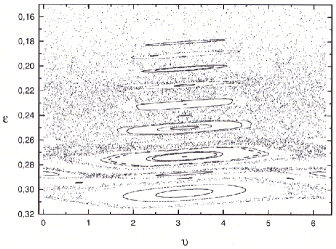
Equations (4) and (6) describe the changes of the energy and phase in time. This map greatly facilitates numerical investigation of dynamics and ionization process. In figures 1 and figureΒ 2 results of the numerical analysis of map (4) - (6) are presented.

Refer to caption
Refer to caption
Figure 2: Ionization threshold field dependence on the relative frequency $s_{0}$. Continuous curve represents results calculated with variation of the initial phase $\vartheta_{0}$, while dotted curve is for $\vartheta_{0}=0$.

3 Two-dimensional atom in monochromatic field

Refer to caption
Figure 3: Two-dimensional atom in the electromagnetic field.

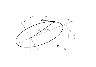
For calculation of the energy change of the arbitrary orientated two-dimensional atom in the electromagnetic field according to equation (3) one should perform the transformation of the coordinates (figureΒ 3). The change of the angular momentum of the atom it follows from the Hamiltonian equations of motion

$$\dot{M}=-\frac{\partial\mathcal{H}}{\partial\alpha}=-rF\sin(\alpha+\varphi)\cos(\omega t+\vartheta)\;.$$ (8)

By analogy with the scaled energy one can introduce the scaled angular momentum $\mu=2M_{s}=2M\omega^{1/3}$. Moreover, it is convenient to introduce the parametric equations of motion for the Coulomb potential [6–8].

Integration of equations (3) and (8) for the half of the period of the electron motion, i.e. for transition from apocenter to pericenter yield the scaled energy and angular momentum changes in the linearly polarized electromagnetic field

Ξ΅j+1=Ξ΅j+2​π​F0​Ρ02Ξ΅j+1{βˆ’[𝐉sβ€²(z)sinΟ‘j+𝐄sβ€²(z)cosΟ‘j]cosΟ†+1βˆ’e2e[(𝐉s(z)βˆ’sin⁑(s​π)s​π)cosΟ‘jβˆ’(𝐄s(z)βˆ’1βˆ’cos⁑(s​π)s​π)sinΟ‘j]sinΟ†}subscriptπœ€π‘—1subscriptπœ€π‘—2πœ‹subscript𝐹0superscriptsubscriptπœ€02subscriptπœ€π‘—1delimited-[]superscriptsubscript𝐉𝑠′𝑧subscriptitalic-ϑ𝑗superscriptsubscript𝐄𝑠′𝑧subscriptitalic-Ο‘π‘—πœ‘1superscript𝑒2𝑒delimited-[]subscriptπ‰π‘ π‘§π‘ πœ‹π‘ πœ‹subscriptitalic-ϑ𝑗subscript𝐄𝑠𝑧1π‘ πœ‹π‘ πœ‹subscriptitalic-Ο‘π‘—πœ‘\varepsilon_{j+1}=\varepsilon_{j}+\frac{2\pi F_{0}\varepsilon_{0}^{2}}{\varepsilon_{j+1}}\left\{-\left[\mathbf{J}_{s}^{\prime}(z)\sin\vartheta_{j}+\mathbf{E}_{s}^{\prime}(z)\cos\vartheta_{j}\right]\cos\varphi\right.\\ \left.+\frac{\sqrt{1-e^{2}}}{e}\left[\left(\mathbf{J}_{s}(z)-\frac{\sin(s\pi)}{s\pi}\right)\cos\vartheta_{j}-\left(\mathbf{E}_{s}(z)-\frac{1-\cos(s\pi)}{s\pi}\right)\sin\vartheta_{j}\right]\sin\varphi\right\}\; (9)

and

ΞΌj+1=ΞΌj+2​π​F0​Ρ02Ξ΅j+1{1βˆ’e2e[(𝐉s(z)βˆ’sin⁑(s​π)s​π)sinΟ‘j+(𝐄s(z)βˆ’1βˆ’cos⁑(s​π)s​π)cosΟ‘j]cosΟ†+[(βˆ’π‰sβ€²(z)+(1+e)sin⁑(s​π)Ο€)cosΟ‘j+(𝐄sβ€²(z)+(1+e)cos⁑(s​π)Ο€+1βˆ’eΟ€)sinΟ‘j]sinΟ†}.subscriptπœ‡π‘—1subscriptπœ‡π‘—2πœ‹subscript𝐹0superscriptsubscriptπœ€02subscriptπœ€π‘—11superscript𝑒2𝑒delimited-[]subscriptπ‰π‘ π‘§π‘ πœ‹π‘ πœ‹subscriptitalic-ϑ𝑗subscript𝐄𝑠𝑧1π‘ πœ‹π‘ πœ‹subscriptitalic-Ο‘π‘—πœ‘delimited-[]superscriptsubscript𝐉𝑠′𝑧1π‘’π‘ πœ‹πœ‹subscriptitalic-ϑ𝑗superscriptsubscript𝐄𝑠′𝑧1π‘’π‘ πœ‹πœ‹1π‘’πœ‹subscriptitalic-Ο‘π‘—πœ‘\mu_{j+1}=\mu_{j}+\frac{2\pi F_{0}\varepsilon_{0}^{2}}{\varepsilon_{j+1}}\left\{\frac{\sqrt{1-e^{2}}}{e}\left[\left(\mathbf{J}_{s}(z)-\frac{\sin(s\pi)}{s\pi}\right)\sin\vartheta_{j}\right.\right.\\ \left.\left.+\left(\mathbf{E}_{s}(z)-\frac{1-\cos(s\pi)}{s\pi}\right)\cos\vartheta_{j}\right]\cos\varphi+\left[\left(-\mathbf{J}_{s}^{\prime}(z)+(1+e)\frac{\sin(s\pi)}{\pi}\right)\cos\vartheta_{j}\right.\right.\\ \left.\left.+\left(\mathbf{E}_{s}^{\prime}(z)+(1+e)\frac{\cos(s\pi)}{\pi}+\frac{1-e}{\pi}\right)\sin\vartheta_{j}\right]\sin\varphi\right\}\;. (10)

Here $\mathbf{E}_{s}(z)$is the Weber function, $z=es$ and e is the eccentricity of the ellipsis. By analogy or from equations (9) and (10) choosing appropriate initial phases of the field one can calculate the energy and angular momentum changes for the electron motion from pericenter to apocenter as well as for the complete period with different initial conditions.

So, for motion between two subsequent passages at the apocenter we have generalization of eq. (4) for the energy change

Ξ΅j+1=Ξ΅j+4​π​F0​Ρ02Ξ΅j+1​{βˆ’π‰s′​(z)​sin⁑ϑj​cos⁑φ+1βˆ’e2e​[𝐉s​(z)βˆ’sin⁑(s​π)s​π]​cos⁑ϑj​sin⁑φ}subscriptπœ€π‘—1subscriptπœ€π‘—4πœ‹subscript𝐹0superscriptsubscriptπœ€02subscriptπœ€π‘—1superscriptsubscript𝐉𝑠′𝑧subscriptitalic-Ο‘π‘—πœ‘1superscript𝑒2𝑒delimited-[]subscriptπ‰π‘ π‘§π‘ πœ‹π‘ πœ‹subscriptitalic-Ο‘π‘—πœ‘\varepsilon_{j+1}=\varepsilon_{j}+\frac{4\pi F_{0}\varepsilon_{0}^{2}}{\varepsilon_{j+1}}\left\{-\mathbf{J}_{s}^{\prime}(z)\sin\vartheta_{j}\cos\varphi+\frac{\sqrt{1-e^{2}}}{e}\left[\mathbf{J}_{s}(z)-\frac{\sin(s\pi)}{s\pi}\right]\cos\vartheta_{j}\sin\varphi\right\}\; (11)

and the angular momentum change

ΞΌj+1=ΞΌj+4​π​F0​Ρ02Ξ΅j+1{1βˆ’e2e[𝐉s(z)βˆ’sin⁑(s​π)s​π]sinΟ‘jcosΟ†+[βˆ’π‰sβ€²(z)+(1+e)sin⁑(s​π)Ο€]cosΟ‘jsinΟ†}.subscriptπœ‡π‘—1subscriptπœ‡π‘—4πœ‹subscript𝐹0superscriptsubscriptπœ€02subscriptπœ€π‘—11superscript𝑒2𝑒delimited-[]subscriptπ‰π‘ π‘§π‘ πœ‹π‘ πœ‹subscriptitalic-Ο‘π‘—πœ‘delimited-[]superscriptsubscript𝐉𝑠′𝑧1π‘’π‘ πœ‹πœ‹subscriptitalic-Ο‘π‘—πœ‘\mu_{j+1}=\mu_{j}+\frac{4\pi F_{0}\varepsilon_{0}^{2}}{\varepsilon_{j+1}}\left\{\frac{\sqrt{1-e^{2}}}{e}\left[\mathbf{J}_{s}(z)-\frac{\sin(s\pi)}{s\pi}\right]\sin\vartheta_{j}\cos\varphi\right.\\ +\left.\left[-\mathbf{J}_{s}^{\prime}(z)+(1+e)\frac{\sin(s\pi)}{\pi}\right]\cos\vartheta_{j}\sin\varphi\right\}\;. (12)

One can calculate the energy and angular momentum changes for the electron motion between two subsequent passages at the pericenter in the similar way.

3.1 Approximation for relatively high frequency $s$

For relatively high frequency of the field, $s\gg 1$, the asymptotic form of the Anger function $\mathbf{J}_{s}(se)$ and its derivative $\mathbf{J}_{s}^{\prime}(se)$ may be used [7]. Then eq. (11) may be written in the form

$$\varepsilon_{j+1}=\varepsilon_{j}+\pi F_{0}\varepsilon_{0}^{2}\left\{(e-2)\left[4b-\frac{4a}{5}\varepsilon_{j+1}-\frac{\sin(\varepsilon_{j+1}^{-3/2}\pi)}{\pi}\varepsilon_{j+1}^{2}\right]\sin\vartheta_{j}\cos\varphi\right.\\ +\frac{\sqrt{1-e^{2}}}{e}\left[4a\varepsilon_{j+1}^{-1/2}-\frac{2\sin(\varepsilon_{j+1}^{-3/2}\pi)}{\pi}\varepsilon_{j+1}^{1/2}-\frac{2b}{35}\varepsilon_{j+1}^{3/2}\right.\\ \left.\left.+(e-1)\left(4b\varepsilon_{j+1}^{-3/2}-\frac{4a}{5}\varepsilon_{j+1}^{-1/2}-\frac{\sin(\varepsilon_{j+1}^{-3/2}\pi)}{\pi}\varepsilon_{j+1}^{1/2}\right)\right]\cos\vartheta_{j}\sin\varphi\right\}\;.$$ (13)

Introducing the generating function we can obtain the iterative equation for the phase $\vartheta_{j}$ as a generalization of eq. (6)

$$\vartheta_{j+1}=\vartheta_{j}+2\pi\varepsilon_{j+1}^{-3/2}+\pi F_{0}\varepsilon_{0}^{2}\left\{(2-e)\left[\frac{4a}{5}-\frac{3\cos(\varepsilon_{j+1}^{-3/2}\pi)}{2}\varepsilon_{j+1}^{-1/2}\right.\right.\\ \left.+\frac{2\sin(\varepsilon_{j+1}^{-3/2}\pi)}{\pi}\varepsilon_{j+1}\right]\cos\vartheta_{j}\cos\varphi+\frac{\sqrt{1-e^{2}}}{e}\left[2a\varepsilon_{j+1}^{-3/2}-3\cos(\varepsilon_{j+1}^{-3/2}\pi)\varepsilon_{j+1}^{-2}\right.\\ +\frac{\sin(\varepsilon_{j+1}^{-3/2}\pi)}{\pi}\varepsilon_{j+1}^{-1/2}+\frac{3b}{35}\varepsilon_{j+1}^{1/2}+(e-1)\left(6b\varepsilon_{j+1}^{-5/2}\right.\\ \left.\left.\left.-2a\varepsilon_{j+1}^{-3/2}-\frac{3\cos(\varepsilon_{j+1}^{-3/2}\pi)}{2}\varepsilon_{j+1}^{-2}+\frac{\sin(\varepsilon_{j+1}^{-3/2}\pi)}{2\pi}\varepsilon_{j+1}^{-1/2}\right)\right]\sin\vartheta_{j}\sin\varphi\right\}\;.$$ (14)
Refer to caption
Refer to caption
Figure 4: Phase plane $(\varepsilon,\vartheta)$ of two-dimensional map (13) and (14) with parameter $\pi F_{0}\varepsilon_{0}^{2}=0.0035$, initial conditions $\vartheta_{0}=\pi$, $\varepsilon_{0}=0.3-0.003i$ ($i=0,1,2,\ldots$) and orientation angle (a) $\varphi=0$ and (b) $\varphi=\pi/6$.

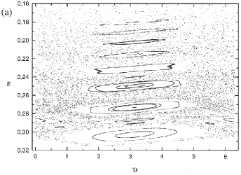
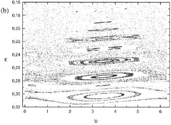
Using mapping equations (13) and (14) we can represent the energy and phase dynamics (figureΒ 4) and calculate numerically the relative threshold field strength for the ionization of the two-dimensional hydrogen atom (figureΒ 5).

Refer to caption
Figure 5: Ionization threshold field dependence on the relative frequency $s_{0}$ for two-dimensional atom with the eccentricity $e=0.9$ and orientation angle $\varphi=0$ (curveΒ 1) and $\varphi=\pi/6$ (curveΒ 2).

3.2 Limiting cases for energy and angular momentum changes

3.2.1 Approximations for very extended orbits

For very extended orbits, $e\rightarrow 1$, the expansions for the energy (11) and angular momentum (12) in powers of $\beta=\sqrt{1-e^{2}}\ll 1$ are

Ξ΅j+1=Ξ΅j+4​π​F0​Ρ02Ξ΅j+1{βˆ’(1+Ξ²2)𝐉sβ€²(s)sinΟ‘jcosΟ†+Ξ²[𝐉s(s)βˆ’sin⁑(s​π)s​π]cosΟ‘jsinΟ†},subscriptπœ€π‘—1subscriptπœ€π‘—4πœ‹subscript𝐹0superscriptsubscriptπœ€02subscriptπœ€π‘—11superscript𝛽2superscriptsubscript𝐉𝑠′𝑠subscriptitalic-Ο‘π‘—πœ‘π›½delimited-[]subscriptπ‰π‘ π‘ π‘ πœ‹π‘ πœ‹subscriptitalic-Ο‘π‘—πœ‘\varepsilon_{j+1}=\varepsilon_{j}+\frac{4\pi F_{0}\varepsilon_{0}^{2}}{\varepsilon_{j+1}}\left\{-\left(1+\beta^{2}\right)\mathbf{J}_{s}^{\prime}(s)\sin\vartheta_{j}\cos\varphi\right.\\ \left.+\beta\left[\mathbf{J}_{s}(s)-\frac{\sin(s\pi)}{s\pi}\right]\cos\vartheta_{j}\sin\varphi\right\}\;, (15)
ΞΌj+1=ΞΌj+4​π​F0​Ρ02Ξ΅j+1{Ξ²[𝐉s(s)βˆ’sin⁑(s​π)s​π]sinΟ‘jcosΟ†+[βˆ’(1+Ξ²2)𝐉sβ€²(s)+(2βˆ’Ξ²2)sin⁑(s​π)Ο€]cosΟ‘jsinΟ†}.subscriptπœ‡π‘—1subscriptπœ‡π‘—4πœ‹subscript𝐹0superscriptsubscriptπœ€02subscriptπœ€π‘—1𝛽delimited-[]subscriptπ‰π‘ π‘ π‘ πœ‹π‘ πœ‹subscriptitalic-Ο‘π‘—πœ‘delimited-[]1superscript𝛽2superscriptsubscript𝐉𝑠′𝑠2superscript𝛽2π‘ πœ‹πœ‹subscriptitalic-Ο‘π‘—πœ‘\mu_{j+1}=\mu_{j}+\frac{4\pi F_{0}\varepsilon_{0}^{2}}{\varepsilon_{j+1}}\left\{\beta\left[\mathbf{J}_{s}(s)-\frac{\sin(s\pi)}{s\pi}\right]\sin\vartheta_{j}\cos\varphi\right.\\ \left.+\left[-\left(1+\beta^{2}\right)\mathbf{J}_{s}^{\prime}(s)+\left(2-\beta^{2}\right)\frac{\sin(s\pi)}{\pi}\right]\cos\vartheta_{j}\sin\varphi\right\}.\; (16)

For $e=1$ eq. (15) coincides with eq. (4) for the one-dimensional atom, while eq. (16) represents change of the angular momentum, resulting to transition to the elliptic states with nonzero angular momentum.

3.2.2 Approximations for almost circular orbits

For almost circular orbits the eccentricity is small, $e\rightarrow 0$. Expansion of expressions (11) and (12) in powers of $e$ may be obtained from equations (3) and (11). The results are

Ξ΅j+1=Ξ΅j+4​F0​Ρ02​sin⁑(s​π)Ξ΅j+1{[e2+34​e2​s2βˆ’11βˆ’s2+12​e​s24βˆ’s2βˆ’34​e2​s29βˆ’s2]sinΟ‘jcosΟ†+s[1βˆ’14​e2​(s2βˆ’4)1βˆ’s2βˆ’e4βˆ’s2+14​e2​s29βˆ’s2]cosΟ‘jsinΟ†},subscriptπœ€π‘—1subscriptπœ€π‘—4subscript𝐹0superscriptsubscriptπœ€02π‘ πœ‹subscriptπœ€π‘—1delimited-[]𝑒234superscript𝑒2superscript𝑠211superscript𝑠212𝑒superscript𝑠24superscript𝑠234superscript𝑒2superscript𝑠29superscript𝑠2subscriptitalic-Ο‘π‘—πœ‘π‘ delimited-[]114superscript𝑒2superscript𝑠241superscript𝑠2𝑒4superscript𝑠214superscript𝑒2superscript𝑠29superscript𝑠2subscriptitalic-Ο‘π‘—πœ‘\varepsilon_{j+1}=\varepsilon_{j}+\frac{4F_{0}\varepsilon_{0}^{2}\sin(s\pi)}{\varepsilon_{j+1}}\left\{\left[\frac{e}{2}+\frac{\frac{3}{4}e^{2}s^{2}-1}{1-s^{2}}+\frac{\frac{1}{2}es^{2}}{4-s^{2}}-\frac{\frac{3}{4}e^{2}s^{2}}{9-s^{2}}\right]\sin\vartheta_{j}\cos\varphi\right.\\[14.22636pt] \left.+s\left[\frac{1-\frac{1}{4}e^{2}(s^{2}-4)}{1-s^{2}}-\frac{e}{4-s^{2}}+\frac{\frac{1}{4}e^{2}s^{2}}{9-s^{2}}\right]\cos\vartheta_{j}\sin\varphi\right\}\;, (17)
ΞΌj+1=ΞΌj+4​F0​Ρ02​sin⁑(s​π)Ξ΅j+1Γ—{s[βˆ’e2+1βˆ’e2​(1+14​s2)1βˆ’s2+e​(1βˆ’12​s2)4βˆ’s2+14​e2​s29βˆ’s2]sinΟ‘jcosΟ†+[3​e2+s2​(12​e2​(1+12​s2)βˆ’1)1βˆ’s2βˆ’12​e​s24βˆ’s2+12​e2​s2​(3βˆ’12​s2)9βˆ’s2]cosΟ‘jsinΟ†}.subscriptπœ‡π‘—1subscriptπœ‡π‘—4subscript𝐹0superscriptsubscriptπœ€02π‘ πœ‹subscriptπœ€π‘—1𝑠delimited-[]𝑒21superscript𝑒2114superscript𝑠21superscript𝑠2𝑒112superscript𝑠24superscript𝑠214superscript𝑒2superscript𝑠29superscript𝑠2subscriptitalic-Ο‘π‘—πœ‘delimited-[]3𝑒2superscript𝑠212superscript𝑒2112superscript𝑠211superscript𝑠212𝑒superscript𝑠24superscript𝑠212superscript𝑒2superscript𝑠2312superscript𝑠29superscript𝑠2subscriptitalic-Ο‘π‘—πœ‘\mu_{j+1}=\mu_{j}+\frac{4F_{0}\varepsilon_{0}^{2}\sin(s\pi)}{\varepsilon_{j+1}}\\ \times\left\{s\left[-\frac{e}{2}+\frac{1-e^{2}(1+\frac{1}{4}s^{2})}{1-s^{2}}+\frac{e(1-\frac{1}{2}s^{2})}{4-s^{2}}+\frac{\frac{1}{4}e^{2}s^{2}}{9-s^{2}}\right]\sin\vartheta_{j}\cos\varphi\right.\\[14.22636pt] \left.+\left[\frac{3e}{2}+\frac{s^{2}(\frac{1}{2}e^{2}(1+\frac{1}{2}s^{2})-1)}{1-s^{2}}-\frac{\frac{1}{2}es^{2}}{4-s^{2}}+\frac{\frac{1}{2}e^{2}s^{2}(3-\frac{1}{2}s^{2})}{9-s^{2}}\right]\cos\vartheta_{j}\sin\varphi\right\}\;. (18)

These expansions are not valid for $s=1,2,3,...$.

4 Atom in the circularly polarized field

The equation for the energy change of the atom in the circularly polarized field is

$$\dot{E_{k}}=-eF\left(v_{x}\cos(\omega t+\vartheta)\pm v_{y}\sin(\omega t+\vartheta)\right)\;.$$ (19)

Here sign $"+"$ or $"-"$ corresponds to the same and opposite directions of the electron and field rotations, respectively.

For the electron, moving between two subsequent pericenter the energy and angular momentum changes are

Ξ΅j+1=Ξ΅jβˆ’4​π​F0​Ρ02Ξ΅j+1​{π‰βˆ’s′​(z)Β±1βˆ’e2e​[π‰βˆ’s​(z)βˆ’sin⁑(s​π)s​π]}​sin⁑(s​π+Ο‘jβˆ“Ο†),subscriptπœ€π‘—1subscriptπœ€π‘—4πœ‹subscript𝐹0superscriptsubscriptπœ€02subscriptπœ€π‘—1plus-or-minussuperscriptsubscript𝐉𝑠′𝑧1superscript𝑒2𝑒delimited-[]subscriptπ‰π‘ π‘§π‘ πœ‹π‘ πœ‹minus-or-plusπ‘ πœ‹subscriptitalic-Ο‘π‘—πœ‘\varepsilon_{j+1}=\varepsilon_{j}-\frac{4\pi F_{0}\varepsilon_{0}^{2}}{\varepsilon_{j+1}}\left\{\mathbf{J}_{-s}^{\prime}(z)\pm\frac{\sqrt{1-e^{2}}}{e}\left[\mathbf{J}_{-s}(z)-\frac{\sin(s\pi)}{s\pi}\right]\right\}\sin(s\pi+\vartheta_{j}\mp\varphi)\;, (20)
ΞΌj+1=ΞΌj+4​π​F0​Ρ02Ξ΅j+1{[1βˆ’e2e(π‰βˆ’s(z)βˆ’sin⁑(s​π)s​π)βˆ“(βˆ’π‰βˆ’sβ€²(z)+(eβˆ’1)sin⁑(s​π)Ο€)]sin(sΟ€+Ο‘jβˆ“Ο†)Β±(1+1/e)​cos⁑(s​π)+1βˆ’1/eΟ€cos(sΟ€+Ο‘jβˆ“Ο†)}.subscriptπœ‡π‘—1subscriptπœ‡π‘—4πœ‹subscript𝐹0superscriptsubscriptπœ€02subscriptπœ€π‘—1plus-or-minusdelimited-[]minus-or-plus1superscript𝑒2𝑒subscriptπ‰π‘ π‘§π‘ πœ‹π‘ πœ‹superscriptsubscript𝐉𝑠′𝑧𝑒1π‘ πœ‹πœ‹minus-or-plusπ‘ πœ‹subscriptitalic-Ο‘π‘—πœ‘11π‘’π‘ πœ‹11π‘’πœ‹minus-or-plusπ‘ πœ‹subscriptitalic-Ο‘π‘—πœ‘\mu_{j+1}=\mu_{j}+\frac{4\pi F_{0}\varepsilon_{0}^{2}}{\varepsilon_{j+1}}\left\{\left[\frac{\sqrt{1-e^{2}}}{e}\left(\mathbf{J}_{-s}(z)-\frac{\sin(s\pi)}{s\pi}\right)\right.\right.\\ \left.\left.\mp\left(-\mathbf{J}_{-s}^{\prime}(z)+(e-1)\frac{\sin(s\pi)}{\pi}\right)\right]\sin(s\pi+\vartheta_{j}\mp\varphi)\right.\\ \left.\pm\frac{(1+1/e)\cos(s\pi)+1-1/e}{\pi}\cos(s\pi+\vartheta_{j}\mp\varphi)\right\}\;. (21)

It should be noted, that expression in the curly brackets in eq. (20) coincides with the expression in the quasiclassical radial dipole matrix element in the velocity representation [6]

DpΒ±=1s​{π‰βˆ’s′​(z)Β±1βˆ’e2e​[π‰βˆ’s​(z)βˆ’sin⁑(s​π)s​π]}.superscriptsubscript𝐷𝑝plus-or-minus1𝑠plus-or-minussuperscriptsubscript𝐉𝑠′𝑧1superscript𝑒2𝑒delimited-[]subscriptπ‰π‘ π‘§π‘ πœ‹π‘ πœ‹D_{p}^{\pm}=\frac{1}{s}\left\{\mathbf{J}_{-s}^{\prime}(z)\pm\frac{\sqrt{1-e^{2}}}{e}\left[\mathbf{J}_{-s}(z)-\frac{\sin(s\pi)}{s\pi}\right]\right\}. (22)

This correspondence, however, takes place only for interaction of the hydrogen atom with the circularly polarized microwave field and for integration of the equations of motion between two subsequent pericenters. In general, the energy [3, 7] and angular momentum changes depend on the integration interval. So, for motion of the electron between two subsequent apocenters, i.e., the most distant from the nucleus points, where the electron’s energy change is minimal, the energy change is described by the expression similar to eq. (20) but instead of $\mathbf{J}_{-s}(es)$ and $\mathbf{J}_{-s}^{\prime}(es)$ we have the Anger function and its derivative of the positive order, $\mathbf{J}_{s}(es)$ and $\mathbf{J}_{s}^{\prime}(es)$. This interval has been used in [3, 4, 5] for derivation of the Kepler map for the one-dimensional hydrogen atom.

5 Conclusion

Analytical expressions for the energy and angular momentum changes of the two-dimensional hydrogen atom in linearly and circularly polarized electromagnetic fields are derived. It should be noted that in general the expressions are rather complicated. The approximate expressions for limiting cases of the parameters are more convenient for analytical and numerical analysis of the dynamics.

The derived expressions are suitable for the three-dimension hydrogen atom as well, and may be generalized for analysis of the chaotic motion (due to the Jupiter perturbations) of comets and asteroids in the Sun system.

References

  • [1] N. B. Delone, V. P. Krainov and D. L. Shepelyansky, Usp. Fiz. Nauk 140, 355 (1983) [Sov. Phys.-Usp. 26, 551 (1983)].
  • [2] P. M. Koch and K. A. H. van Leeuwen, Phys. Rep., V. 255 , 289 (1995).
  • [3] V. Gontis and B. Kaulakys, J. Phys. B: At. Mol. Opt. Phys., V. 20, 5051 (1987).
  • [4] B. Kaulakys and G. Vilutis, Phys. Scripta, V. 59, 251 (1999) .
  • [5] B. Kaulakys, D. Grauzhinis and G. Vilutis, Europhys. Lett., V. 43, 123 (1998).
  • [6] B. Kaulakys, J. Phys. B: At. Mol. Opt. Phys., V. 28, 4963 (1995).
  • [7] B. Kaulakys, J. Phys. B: At. Mol. Opt. Phys., V. 24, 571 (1991).
  • [8] L. D. Landau and E. M. Lifshitz, Classical Field Theory (Pergamon, New York, 1975).
  • [9] A. J. Lichtenberg and M. A. Lieberman, Regular and Stochastic Motion (Springer-Verlag, New York, 1983 and 1992).
  • [10] G. M. Zaslavskii, Stochastic Behavior of Dynamical Systems (Nauka, Moscow, 1984; Harwood, New York, 1985).