Thermodynamic functions of dense plasmas: analytic approximations for astrophysical applications

Abstract.

We briefly review analytic approximations of thermodynamic functions of fully ionized nonideal electron-ion plasmas, applicable in a wide range of plasma parameters, including the domains of nondegenerate and degenerate, nonrelativistic and relativistic electrons, weakly and strongly coupled Coulomb liquids, classical and quantum Coulomb crystals. We present improvements to previously published approximations. Our code for calculation of thermodynamic functions based on the reviewed approximations is made publicly available.

1. Introduction

In a previous work [1, 2], we performed hypernetted chain (HNC) calculations and proposed analytic formulae for the equation of state (EOS) of electron-ion plasmas (EIP). An alternative analytic approximation for the EOS of EIP was proposed in [3, 4]. A comparison (e.g., [1, 4]) shows that the formulae in [2] have a higher accuracy, in particular for the thermodynamic contributions of ion-ion and ion-electron correlations in the regime of moderate Coulomb coupling. Recently [5, 6], we studied classical ion mixtures and proposed a correction to the linear mixing rule. In this paper we review the analytic expressions for all contributions to thermodynamic functions and introduce some practical modifications to the previously published formulae. The reviewed analytic description of the thermodynamic functions of Coulomb plasmas is realized in a publicly available computer code.

Let $n_{e}$ and $n_{\mathrm{i}}$ be the electron and ion number densities, $A$ and $Z$ the ion mass and charge numbers, respectively. The electric neutrality implies $n_{e}=Zn_{\mathrm{i}}$. In this paper we neglect positrons (they can be described using the same formulae as the electrons; see, e.g., Ref. [7]) and free neutrons (see, e.g., Ref. [8]), and consider mainly plasmas containing a single type of ions (for the extension to multicomponent mixtures, see [5, 6]).

The state of a free electron gas is determined by the electron number density $n_{e}$ and temperature $T$. Instead of $n_{e}$ it is convenient to introduce the dimensionless density parameter $r_{s}=a_{e}/a_{0}$, where $a_{0}$ is the Bohr radius and $a_{e}=(\frac{4}{3}\pi n_{e})^{-1/3}$. The parameter $r_{s}$ can be easily evaluated from the relations $r_{s}=1.1723\,n_{24}^{-1/3},$ where $n_{24}\equiv n_{e}/10^{24}{\rm~{}cm}^{-3}$, or $r_{s}=(\rho_{0}/\rho)^{1/3},$ where $\rho_{0}=2.6752\,(A/Z)$ g cm^-3. The analogous density parameter for the ion one-component plasma (OCP) is $R_{S}=a_{\mathrm{i}}m_{\mathrm{i}}(Ze)^{2}/\hbar^{2}=1822.89\,r_{s}AZ^{7/3}$, where $m_{\mathrm{i}}$ is the ion mass and $a_{\mathrm{i}}\equiv(\frac{4}{3}\pi n_{\mathrm{i}})^{-1/3}=a_{e}Z^{1/3}$ is the ion sphere radius.

At stellar densities it is convenient to use, instead of $r_{s}$, the relativity parameter [9] $x_{\mathrm{r}}=p_{\mathrm{F}}/m_{e}c=1.00884\,\left(\rho_{6}Z/A\right)^{1/3}\!\!=0.014005\,r_{s}^{-1},$ where $p_{\mathrm{F}}=\hbar\,(3\pi^{2}n_{e})^{1/3}$ is the electron Fermi momentum and $\rho_{6}\equiv\rho/10^{6}$ g cm^-3. The Fermi kinetic energy is $\epsilon_{\mathrm{F}}=c\,\sqrt{(m_{e}c)^{2}+p_{\mathrm{F}}^{2}}-m_{e}c^{2},$ and the Fermi temperature equals $T_{\mathrm{F}}\equiv\epsilon_{\mathrm{F}}/k_{B}=T_{\mathrm{r}}\,(\gamma_{\mathrm{r}}-1),$ where $T_{\mathrm{r}}\equiv{m_{e}c^{2}/k_{B}}=5.93\times 10^{9}~{}\mathrm{K}$, $\gamma_{\mathrm{r}}\equiv\sqrt{1+x_{\mathrm{r}}^{2}}$, and $k_{B}$ is the Boltzmann constant. If $x_{\mathrm{r}}\ll 1$, then $T_{\mathrm{F}}\approx 1.163\times 10^{6}\,r_{s}^{-2}$ K. The effects of special relativity are controlled by $x_{\mathrm{r}}$ in degenerate plasmas ($T\ll T_{\mathrm{F}}$) and by $\tau\equiv{T/T_{\mathrm{r}}}$ in nondegenerate plasmas ($T\gg T_{\mathrm{F}}$).

The ions are nonrelativistic in most applications. The strength of the Coulomb interaction of ions is characterized by the Coulomb coupling parameter $\Gamma={(Ze)^{2}}/{a_{\mathrm{i}}k_{B}T}=\Gamma_{e}Z^{5/3},$ where $\Gamma_{e}\equiv{e^{2}}/{a_{e}k_{B}T}\approx{22.747}\,{T_{6}^{-1}}\left(\rho_{6}{Z}/{A}\right)^{1/3}$ and $T_{6}\equiv T/10^{6}$ K.

Thermal de Broglie wavelengths of the ions and electrons are usually defined as $\lambda_{\mathrm{i}}=\left({2\pi\hbar^{2}}/{m_{\mathrm{i}}k_{B}T}\right)^{1/2}$ and $\lambda_{e}=\left({2\pi\hbar^{2}}/{m_{e}k_{B}T}\right)^{1/2}.$ The quantum effects on ion motion are important either at $\lambda_{\mathrm{i}}\gtrsim a_{\mathrm{i}}$ or at $T\ll T_{\mathrm{p}}$, where $T_{\mathrm{p}}\equiv(\hbar\omega_{\mathrm{p}}/k_{B})\approx 7.832\times 10^{6}\,(Z/A)\,\sqrt{\rho_{6}}\,\textrm{~{}K}$ is the plasma temperature determined by the ion plasma frequency $\omega_{\mathrm{p}}=\left({4\pi e^{2}\,n_{\mathrm{i}}}Z^{2}/m_{\mathrm{i}}\right)^{1/2}.$ The corresponding dimensionless parameter is $\eta\equiv T_{\mathrm{p}}/T$.

Assuming commutativity of the kinetic and potential energy operators and separation of the traces of the electronic and ionic parts of the Hamiltonian, the total Helmholtz free energy $F$ can be conveniently written as $F=F_{\mathrm{id}}^{(i)}+F_{\mathrm{id}}^{(e)}+F_{ee}+F_{\mathrm{ii}}+F_{ie},$ where $F_{\mathrm{id}}^{(i)}$ and $F_{\mathrm{id}}^{(e)}$ denote the ideal free energy of ions and electrons, and the last three terms represent an excess free energy arising from the electron-electron, ion-ion, and ion-electron interactions, respectively. This decomposition induces analogous decompositions of pressure $P$, internal energy $U$, entropy $S$, the heat capacity $C_{V}$, and the pressure derivatives $\chi_{T}=(\partial\ln P/\partial\ln T)_{V}$ and $\chi_{\rho}=-(\partial\ln P/\partial\ln V)_{T}.$ Other second-order functions can be expressed through these ones by Maxwell relations.

2. Ideal part of the free energy

The free energy of a gas of $N_{\mathrm{i}}=n_{\mathrm{i}}V$ nonrelativistic classical ions is $F_{\mathrm{id}}^{(i)}=N_{\mathrm{i}}k_{B}T\left[\ln(n_{\mathrm{i}}\lambda_{\mathrm{i}}^{3}/M)-1\right],$ where $M$ is the spin multiplicity. In the OCP, it can be written in terms of the dimensionless plasma parameters as ${F_{\mathrm{id}}^{(i)}}={N_{\mathrm{i}}k_{B}T}\left[3\ln\eta-1.5\ln\Gamma-0.5\ln(6/\pi)-\ln M-1\right].$

The free energy of the electron gas is given by $F_{\mathrm{id}}^{(e)}=\mu_{e}N_{e}-P_{\mathrm{id}}^{(e)}\,V,$ where $\mu_{e}$ is the electron chemical potential. The pressure and the number density are functions of $\mu_{e}$ and $T$:

$$P_{\mathrm{id}}^{(e)}=\frac{8}{3\sqrt{\pi}}\,\frac{k_{B}T}{\lambda_{e}^{3}}\left[I_{3/2}(\chi_{e},\tau)+\frac{\tau}{2}I_{5/2}(\chi_{e},\tau)\right],\quad n_{e}=\frac{4}{\sqrt{\pi}\,\lambda_{e}^{3}}\left[I_{1/2}(\chi_{e},\tau)+\tau I_{3/2}(\chi_{e},\tau)\right],$$ (1)

where $\chi_{e}=\mu_{e}/k_{B}T$ (here, we do not include the rest energy $m_{e}c^{2}$ in $\mu_{e}$) and

$$I_{\nu}(\chi_{e},\tau)\equiv\int_{0}^{\infty}\frac{x^{\nu}\,(1+\tau x/2)^{1/2}}{\exp(x-\chi_{e})+1}\,{\mathrm{d}}x$$ (2)

is a Fermi-Dirac integral. An analytic approximation for $\mu_{e}(n_{e})$ has been derived in [1].

In Ref. [1] we calculated $I_{\nu}(\chi_{e},\tau)$ using analytical approximations [7]. These approximations are piecewise: below, within, and above the interval $0.6\leq\chi_{e}<14$. Their typical fractional accuracy is a few $\times 10^{-4}$, the maximum error and discontinuities at the boundaries reach $\sim 0.2$%. For the first and second derivatives, the errors and discontinuities lie within 1.5%. At $\chi_{e}\geq 14$ we use the Sommerfeld expansion (e.g., [10])

$$I_{\nu}(\chi_{e},\tau)\approx\mathcal{I}_{\nu}^{(0)}(\tilde{\mu})+\frac{\pi^{2}}{6}\tau^{2}\mathcal{I}_{\nu}^{(2)}(\tilde{\mu})+\frac{7\pi^{4}}{360}\tau^{4}\mathcal{I}_{\nu}^{(4)}(\tilde{\mu})+\ldots,$$ (3)

where we have defined $\tilde{\mu}=\chi_{e}\tau=\mu_{e}/m_{e}c^{2}$,

$$\mathcal{I}_{\nu}^{(0)}(\epsilon)=\int_{0}^{\epsilon}\mathcal{I}_{\nu}^{(1)}(\epsilon^{\prime})\,\mathrm{d}\epsilon^{\prime}=\int_{0}^{x_{0}}\big{(}\sqrt{1+x^{2}}-1\big{)}^{\nu-1/2}\frac{x^{2}\,\mathrm{d}x}{\sqrt{1+x^{2}}},\quad\mathcal{I}_{\nu}^{(n+1)}(\tilde{\mu})=\frac{\mathrm{d}\mathcal{I}_{\nu}^{(n)}(\tilde{\mu})}{\mathrm{d}\tilde{\mu}},$$ (4)

$\mathcal{I}_{\nu}^{(1)}(\epsilon)=\epsilon^{\nu}\sqrt{2+\epsilon}$ and $x_{0}\equiv\sqrt{\tilde{\mu}(2+\tilde{\mu})}$. In particular,

$$\mathcal{I}_{1/2}^{(0)}(\tilde{\mu})=[x_{0}\gamma_{0}-\ln(x_{0}+\gamma_{0})]/2,\quad\mathcal{I}_{3/2}^{(0)}(\tilde{\mu})=x_{0}^{3}/3-\mathcal{I}_{1/2}^{(0)}(\tilde{\mu}),\quad\mathcal{I}_{5/2}^{(0)}(\tilde{\mu})=x_{0}^{3}\gamma_{0}/4-2x_{0}^{3}/3+1.25\,\mathcal{I}_{1/2}^{(0)}(\tilde{\mu}),$$

where $\gamma_{0}\equiv\sqrt{1+x_{0}^{2}}=1+\tilde{\mu}\,$ (note that, if $\tilde{\mu}=\tilde{\epsilon}$, where $\tilde{\epsilon}\equiv\epsilon_{\mathrm{F}}/m_{e}c^{2}$, then $x_{0}=x_{\mathrm{r}}$ and $\gamma_{0}=\gamma_{\mathrm{r}}$).

At small $\tilde{\mu}$, accuracy can be lost because of numerical cancellations of close terms of opposite signs in Eq. (3) and in the respective partial derivatives. In this case we use the expansion

$$I_{\nu}(\chi,\tau)=\!I^{\mathrm{nr}}_{\nu}(\chi)+\!\sum_{m=0}^{\infty}(-1)^{m}\frac{(2m-1)!!\,\tau^{m+1}}{4^{m+1}m!}I^{\mathrm{nr}}_{\nu+m+1}(\chi),\quad I^{\mathrm{nr}}_{\nu}(\chi)=\int_{0}^{\infty}\frac{x^{\nu}\,\mathrm{d}x}{e^{x-\chi}+1},$$ (5)

where $(2m-1)!!\equiv\prod_{k=1}^{m}(2k-1)$ should be replaced by 1 for $m=0$. At large $\chi$, the nonrelativistic Fermi integrals $I^{\mathrm{nr}}_{\nu}(\chi)$ are calculated with the use of the Sommerfeld expansion. Sufficiently smooth and accurate overall approximations for functions $I_{\nu}(\chi_{e},\tau)$ with $\nu=\frac{1}{2}$, $\frac{3}{2}$, and $\frac{5}{2}$ are provided by switching to Eq. (5) at $\chi_{e}\geq 14$ and $\tilde{\mu}<0.1$, while retaining the terms up to $m=3$.

The chemical potential at fixed $n_{e}$ is obtained with fractional accuracy $\sim T^{2}/T_{\mathrm{F}}^{2}\,$ by using Eqs. (1), (3), setting $\mathcal{I}_{\nu}^{(n)}(\tilde{\mu})\approx\mathcal{I}_{\nu}^{(n)}(\tilde{\epsilon})+\mathcal{I}_{\nu}^{(n+1)}(\tilde{\epsilon})\,(\tilde{\mu}-\tilde{\epsilon}),$ and dropping the terms that contain the product $(\tilde{\mu}-\tilde{\epsilon})\,\tau^{2}$. Then at $T\ll T_{\mathrm{F}}$

$$\Delta\tilde{\epsilon}\equiv\tilde{\epsilon}-\tilde{\mu}\approx\frac{\pi^{2}\tau^{2}}{6\,\tilde{\epsilon}}\,\frac{1+2x_{\mathrm{r}}^{2}}{\gamma_{\mathrm{r}}(1+\gamma_{\mathrm{r}})}\,,\quad\Delta F\equiv F_{\mathrm{id}}^{(e)}-F_{0}^{(e)}\approx-\frac{1}{2}\,TS_{\mathrm{id}}^{(e)}\approx-P_{\mathrm{r}}V\frac{x_{\mathrm{r}}\gamma_{\mathrm{r}}\tau^{2}}{6},$$ (6)

where $F_{0}^{(e)}=({P_{\mathrm{r}}V}/{8\pi^{2}})[x_{\mathrm{r}}\,(1+2x_{\mathrm{r}}^{2})\,\gamma_{\mathrm{r}}-\ln(x_{\mathrm{r}}+\gamma_{\mathrm{r}})]-N_{e}m_{e}c^{2}$ is the zero-temperature limit [11] (without the rest energy $N_{e}m_{e}c^{2}$), and $P_{\mathrm{r}}\equiv m_{e}c^{2}\,(m_{e}c/\hbar)^{3}=1.4218\times 10^{25}\mathrm{~{}dyn~{}cm}^{-2}$ is the relativistic unit of pressure.

Accordingly, $P_{\mathrm{id}}^{(e)}\approx P_{0}^{(e)}+\Delta P,$ where $P_{0}^{(e)}=({P_{\mathrm{r}}}/{8\pi^{2}})\,\left[x_{\mathrm{r}}\left(\frac{2}{3}\,x_{\mathrm{r}}^{2}-1\right)\gamma_{\mathrm{r}}+\ln(x_{\mathrm{r}}+\gamma_{\mathrm{r}})\right],$ and $\Delta P=(P_{\mathrm{r}}/18)\,\tau^{2}x_{\mathrm{r}}\,(2+x_{\mathrm{r}}^{2})/\gamma_{\mathrm{r}}$. In this case, $\chi_{\rho}^{(e)}\approx P_{\mathrm{r}}x_{\mathrm{r}}^{5}/9\pi^{2}\gamma_{\mathrm{r}}P_{\mathrm{id}}^{(e)},$ $\chi_{T}^{(e)}\approx 2\Delta P/P_{\mathrm{id}}^{(e)},$ $C_{V}^{(e)}\approx\pi^{2}k_{B}N_{e}\,\gamma_{\mathrm{r}}\tau/x_{\mathrm{r}}^{2}.$ In order to minimize numerical jumps at the transition between the fit at $\chi_{e}<14$ and the Sommerfeld expansion at $\chi_{e}>14$, we multiply the expressions for $\Delta F$ by empirical correction factor $(1+\Delta\tilde{\epsilon}/\tilde{\epsilon})^{-1}$, and those for $\chi_{T}^{(e)}$ and $C_{V}^{(e)}$ by $[1+(4-2x_{\mathrm{r}}/\gamma_{\mathrm{r}})\,\Delta\tilde{\epsilon}/\tilde{\epsilon}]^{-1}$.

At $x_{\mathrm{r}}<10^{-5}$ we replace $F_{0}^{(e)}$ and $P_{0}^{(e)}$ by their nonrelativistic limits, $F_{0}^{(e)}/V=P_{\mathrm{r}}x_{\mathrm{r}}^{5}/10\pi^{2}$ and $P_{0}^{(e)}=P_{\mathrm{r}}x_{\mathrm{r}}^{5}/15\pi^{2}\propto n_{e}^{5/3}$. In the opposite case of $x_{\mathrm{r}}\gg 1$, one has $P_{0}^{(e)}=P_{\mathrm{r}}x_{\mathrm{r}}^{4}/12\pi^{2}\propto n_{e}^{4/3}$.

3. Electron exchange and correlation

Electron exchange-correlation effects were studied by many authors. For the reasons explained in [1], we adopt the fit to $F_{ee}$ presented in Ref. [12]. It is valid at any densities and temperatures, provided that $x_{\mathrm{r}}\ll 1$.

In Ref. [2] we implemented an interpolation between the nonrelativistic fit [12] and approximation [3, 4] valid for strongly degenerate relativistic electrons. However, later on we found that such an interpolation may cause an unphysical behavior of the heat capacity in a certain density-temperature domain. Therefore we have reverted to the original formula [12], taking into account that in applications, as long as the electrons are relativistic, their exchange and correlation contributions are orders of magnitude smaller than the other contributions to the EOS of EIP (see, e.g., [13, 8]).

4. One-component plasma

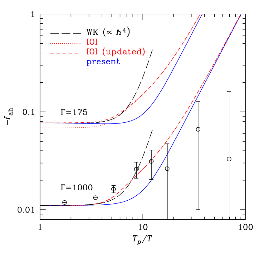
Figure 1. Anharmonic contribution to the reduced free energy of an ion lattice as a function of the quantum parameter $\eta=T_{\mathrm{p}}/T$ for two values of the Coulomb coupling parameter, $\Gamma=175$ (upper curves) and 1000 (lower curves). A comparison of different approximations (see text): Wigner expansion (long-dashed lines); an approximation from [25] (IOI, dotted lines); the same approximation with the coefficients adjusted to Ref. [21] (short-dashed lines); and present interpolation (8) (solid lines). The points with errorbars show simulation results from [25] for $\Gamma=1000$.

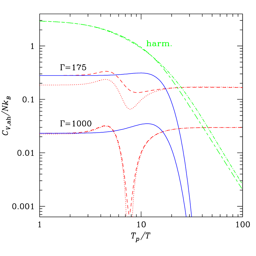
Figure 2. Harmonic and anharmonic lattice contributions to the reduced heat capacity at $\Gamma=175$ and 1000. The harmonic lattice contribution according to Ref. [20] (dot-dashed lines) is compared to the model [18] (long-short-dash lines) and to the anharmonic correction in different approximations (see text): a derivative of the IOI fit [25] (dotted lines: original; short-dashed lines: improved; see text) and a corresponding derivative of Eq. (8) (solid lines).

4.1. Coulomb liquid

For the reduced free energy of the ion-ion interaction $f_{\mathrm{ii}}\equiv{F_{\mathrm{ii}}}/{N_{\mathrm{i}}k_{B}T}$ in the liquid OCP at any values of $\Gamma$ we use the analytic approximation derived in Ref. [2]. In order to extend its applicability range from $T\gg T_{\mathrm{p}}$ to $T\sim T_{\mathrm{p}}$, we add the lowest-order quantum corrections to the Helmholtz free energy [14]: $f_{q}^{(2)}=\eta^{2}/24.$ The next-order correction $\propto\hbar^{4}$ has been obtained in [15]. These corrections have limited applicability, because as soon as $\eta$ becomes large, the Wigner expansion diverges and the plasma forms a quantum liquid, whose free energy is not known in an analytic form.

A classical OCP freezes at temperature $T_{\mathrm{m}}$ corresponding to $\Gamma=175$, but in real plasmas $T_{\mathrm{m}}$ is affected by electron polarization [2, 16] and quantum effects (e.g., [17, 18, 19]). Hence the liquid does not freeze, regardless of $T$, at densities larger than the critical one. The critical density values in the OCP correspond to $R_{S}\approx 140$ – 160 for bosons and $R_{S}\approx 90$ – 110 for fermions. In astrophysical applications, the appearance of quantum liquid can be important for hydrogen and helium plasmas (see, e.g., Ref. [18] for discussion).

4.2. Coulomb crystal

The reduced free energy of the Coulomb crystal is $f_{\mathrm{lat}}\equiv F_{\mathrm{lat}}/N_{\mathrm{i}}k_{B}T=C_{0}\Gamma+1.5u_{1}\eta+f_{\mathrm{th}}+f_{\mathrm{ah}}.$ Here, the first term is the Madelung energy ($C_{0}\approx-0.9$), the second represents zero-point ion vibrations energy ($u_{1}\approx 0.5$), $f_{\mathrm{th}}$ is the thermal correction in the harmonic approximation, and $f_{\mathrm{ah}}$ is the anharmonic correction. We use the most accurate values of $C_{0}$, $u_{1}$, and analytic approximations to $f_{\mathrm{th}}$ for bcc and fcc Coulomb OCP lattices, which have been obtained in [20].

For the classical anharmonic corrections, 11 fitting expressions were given in [21]. We have chosen one of them: $f_{\mathrm{ah}}^{(0)}(\Gamma)=a_{1}/\Gamma+a_{2}/2\Gamma^{2}+a_{3}/3\Gamma^{3},$ with $a_{1}=10.9$, $a_{2}=247$, and $a_{3}=1.765\times 10^{5}$, because this choice is most consistent with the perturbation theory [17, 22].

In applications one needs a continuous extension for the free energy to $\eta\neq 0$. With the leading quantum anharmonic correction at small $\eta$ one has [15]

$$f_{\mathrm{ah}}\approx f_{\mathrm{ah}}^{(0)}(\Gamma)-(0.0018/\Gamma+0.085/\Gamma^{2})\,\eta^{4}.$$ (7)

At $T\to 0$, the quantum anharmonic corrections were studied in [23, 24, 17], where an expansion in powers of $R_{S}^{-1/2}$ was obtained, assuming $R_{S}\gg 1$. The leading term of this expansion can be written in the form $f_{\mathrm{ah},T\to 0}=-b_{1}\eta^{2}/\Gamma.$ In the literature one finds different estimates for $b_{1}$; we use $b_{1}=0.12$ as an approximation consistent with [23, 24]. Free and internal energies of finite-temperature quantum crystals were calculated using quantum Monte Carlo methods in [25, 19, 26]. Iyetomi et al. in Ref. [25] (hereafter IOI) proposed an analytic expression for the quantum anharmonic corrections. However, differences between the numerical results in [25, 19, 26] are comparable to the differences between the numerical results and the harmonic approximation. Therefore, finite-temperature anharmonic corrections cannot be accurately determined from the listed results.

In order to reproduce the zero-temperature and classical limits, we multiply $f_{\mathrm{ah}}^{(0)}$ by exponential suppression factor $e^{-c_{1}\eta^{2}}$ and add $f_{\mathrm{ah},T\to 0}$. Then we have

$$f_{\mathrm{ah}}=f_{\mathrm{ah}}^{(0)}(\Gamma)\,e^{-c_{1}\eta^{2}}-b_{1}\eta^{2}/\Gamma.$$ (8)

According to Eq. (7), the Taylor expansion coefficient at $\eta^{2}/\Gamma$ equals zero. In order to reproduce this property, we set $c_{1}=b_{1}/a_{1}\approx 0.0112$. In Fig. 2, the resulting approximation for the free energy as a function of $\eta$ (solid lines) is compared to the semiclassical expression [Eq. (7); long-dashed lines] and to the elaborated IOI fitting formula: the dotted lines correspond to the original coefficients of this fit, chosen by IOI so as to reproduce the results of Ref. [22] at $\eta\to 0$, while the short-dashed curves show the same fit, but with the coefficients adjusted to more recent results [21] at $\eta\to 0$. The curves of the two latter types nearly coincide at $\Gamma=1000$, but differ near the melting point $\Gamma=175$.

Interpolation (8) (unlike, for example, Padé approximations [27]) does not produce an unphysical behavior of thermodynamic functions. In particular, anharmonic corrections to the heat capacity and entropy do not exceed the reference (harmonic-lattice) values of these quantities at any $\eta$. In Fig. 2, we show the ion contributions to the reduced heat capacity of the ion lattice $c_{V,i}\equiv C_{V,i}/N_{\mathrm{i}}k_{B}$, calculated through derivatives of Eq. (8) (solid lines), and compare it to the contributions calculated through derivatives of the fitting formula in [25] (short-dashed and dotted lines). In the same figure we plot the harmonic-crystal contribution to the reduced heat capacity: the short-dash–long-dash line corresponds to the model of Ref. [18] (which we adopted in [2]), while the dot-dashed line corresponds to the most accurate formula [20].

Interpolation Eq. (8) should be replaced by a more accurate formula in the future when accurate finite-temperature anharmonic quantum corrections become available.

5. Electron polarization

5.1. Coulomb liquid

Electron polarization in Coulomb liquid was studied by perturbation [28, 13] and HNC [29, 30, 1, 2] techniques. The results for $F_{ie}$ are fitted by analytic expressions in [2]. This fit is accurate within several percents, and it exactly recovers the Debye-Hückel limit for EIP at $\Gamma\to 0$ and the Thomas-Fermi result [9] at $\Gamma\gg 1$ and $Z\gg 1$.

5.2. Coulomb crystal

Calculation of thermodynamic functions for a Coulomb crystal with allowance for the electron polarization is a complex problem. For classical ions, the simplest screening model consists in replacing the Coulomb potential by the Yukawa potential. For instance, there were molecular dynamics simulations of classical Yukawa systems [16] and path-integral Monte Carlo simulations of a quantum Yukawa crystal at $R_{S}=200$ [31]. However, the Yukawa interaction reflects only the small-wavenumber asymptote of the electron dielectric function. A rigorous treatment would consist in calculating the dynamical matrix and solving a corresponding dispersion relation for the phonon spectrum. The first-order perturbation approximation for the dynamical matrix of a classical Coulomb solid with the polarization corrections was developed in Ref. [32]. The phonon spectrum in such a quantum crystal has been calculated only in the harmonic approximation [33], which has a restricted applicability: for example, it cannot reproduce the known classical ($T\gg T_{\mathrm{p}}$) limit of the anharmonic $ie$ contribution to the heat capacity.

A semiclassical perturbation approach was used in [2]. The results were fitted by the analytic expression

$$f_{ie}=-f_{\infty}(x_{\mathrm{r}})\,\Gamma\left[1+A(x_{\mathrm{r}})\,(Q(\eta)/\Gamma)^{s}\right].$$ (9)

In the classical Coulomb crystal, $Q=1$, $f_{\infty}(x)=b_{1}\,\sqrt{1+b_{2}/x^{2}},$ and $A(x)=(b_{3}+a_{3}x^{2})/(1+b_{4}x^{2})$. Parameters $s$ and $b_{1}$–$b_{4}$ depend on $Z$ and are chosen so as to fit the perturbational results; $a_{3}$ is a constant. All the parameters weakly depend on the lattice type; they are explicit in [2] for the bcc and fcc lattices.

The factor $Q(\eta)$ in Eq. (9) is designed to reproduce the suppression of the dependence of $F_{ie}$ on $T$ at $T\ll T_{\mathrm{p}}$. For the classical solid, $Q(0)=1$. In the quantum limit ($\eta\to\infty$) $Q(\eta)\simeq q\eta$, so that the ratio $Q/\Gamma$ in Eq. (9) becomes independent of $T$. The proportionality coefficient $q$ was found numerically in [2]; it equals 0.205 for the bcc lattice.

The form of $Q(\eta)$ suggested in [2] assumed a too slow decrease of the heat capacity ($C_{V,ie}\propto\eta^{-1}\propto T$) at $\eta\to\infty$, which signals the violation of the employed semiclassical perturbation theory in the strong quantum limit, related to the approximate form of the ion structure factor used in the calculations, as discussed in [2, 8]. In order to fix this problem, we have changed the form of $Q(\eta)$ to

$$Q(\eta)=\left[{\ln\left(1+e^{(q\eta)^{2}}\right)}\right]^{1/2}\,\left[{\ln\left(e-(e-2)e^{-(q\eta)^{2}}\right)}\right]^{-1/2}.$$ (10)

This form of $Q(\eta)$ has the correct limits at $\eta\to 0$ and $\eta\to\infty$ and is compatible with the numerical results [2]. In addition, it eliminates the problematic $ie$ contributions to the heat capacity and entropy at $\eta\gg 1$. It can be improved in the future when the polarization corrections for the quantum Coulomb crystal are accurately evaluated.

6. Conclusions

We have reviewed analytic approximations for the EOS of fully ionized electron-ion plasmas and described recent improvements to the previously published approximations, taking into account nonideality due to ion-ion, electron-electron, and electron-ion interactions. The presented formulae are applicable in a wide range of plasma parameters, including the domains of nondegenerate and degenerate, nonrelativistic and relativistic electrons, weakly and strongly coupled Coulomb liquids, classical and quantum Coulomb crystals.

For brevity we have considered plasmas composed of electrons and one type of ions. Extension to the case where several types of ions are present is provided by [5, 6].

We have made the Fortran code that realizes the analytical approximations for the free energy and its derivatives, described in this paper, freely available in the Internet .

The work of A.Y.P. was partially supported by the Rosnauka Grant NSh-2600.2008.2 and the RFBR Grant 08-02-00837, and by CompStar, a Research Networking Programme of the European Science Foundation.

References

- [1] G. Chabrier and A. Y. Potekhin, Phys. Rev. E 58, 4941 (1998).
- [2] A. Y. Potekhin and G. Chabrier, Phys. Rev. E 62, 8554 (2000).
- [3] W. Stolzmann and T. Blöcker, Phys. Lett. A 221, 99 (1996).
- [4] W. Stolzmann and T. Blöcker, Astron. Astrophys. 361, 1152 (2000).
- [5] A. Y. Potekhin, G. Chabrier, and F. J. Rogers, Phys. Rev. E 79, 016411 (2009).
- [6] A. Y. Potekhin, G. Chabrier, A. I. Chugunov, H. E. DeWitt, and F. J. Rogers, Phys. Rev. E 80, 047401 (2009).
- [7] S. I. Blinnikov, N. V. Dunina-Barkovskaya, and D. K. Nadyozhin, Astrophys. J. Suppl. Ser. 106 171 (1996); erratum: ibid. 118, 603 (1998).
- [8] P. Haensel, A. Y. Potekhin, and D. G. Yakovlev, Neutron Stars 1: Equation of State and Structure (Springer, New York, 2007).
- [9] E. E. Salpeter, Astrophys. J. 134, 669 (1961).
- [10] S. Chandrasekhar, An Introduction to the Study of Stellar Structure (University of Chicago Press, Chicago, 1939; Dover, New York, 1957), Chap. X.
- [11] J. Frenkel, Z. f. Physik 50, 234 (1928).
- [12] S. Ichimaru, H. Iyetomi, and S. Tanaka, Phys. Rep. 149, 91 (1987).
- [13] D. G. Yakovlev and D. A. Shalybkov, Sov. Astron. Lett. 13, 308 (1987); Astrophys. Space Phys. Rev. 7, 311 (1989).
- [14] J. P. Hansen, Phys. Rev. A 8, 3096 (1973).
- [15] J. P. Hansen and P. Vieillefosse, Phys. Lett. A 53, 187 (1975).
- [16] S. Hamaguchi, R. T. Farouki, and D. H. E. Dubin, Phys. Rev. E 56, 4671 (1997).
- [17] H. Nagara, Y. Nagata, and T. Nakamura, Phys. Rev. A 36, 1859 (1987).
- [18] G. Chabrier, Astrophys. J. 414 695 (1993).
- [19] M. D. Jones and D. M. Ceperley, Phys. Rev. Lett. 76, 4572 (1996).
- [20] D. A. Baiko, A. Y. Potekhin, and D. G. Yakovlev, Phys. Rev. E 64, 057402 (2001).
- [21] R. T. Farouki and S. Hamaguchi, Phys. Rev. E 47, 4330 (1993).
- [22] D. H. E. Dubin, Phys. Rev. A 42, 4972 (1990).
- [23] W. J. Carr, Jr., R. A. Coldwell-Horsfall, and A. E. Fein, Phys. Rev. 124, 747 (1961).
- [24] R. C. Albers and J. E. Gubernatis, Phys. Rev. B 33, 5180 (1986); erratum: ibid. 42, 11373 (1990).
- [25] H. Iyetomi, S. Ogata, and S. Ichimaru, Phys. Rev. B 47, 11703 (1993).
- [26] G. Chabrier, F. Douchin, and A. Y. Potekhin, J. Phys.: Condens. Matter 14, 9133 (2002).
- [27] A. I. Chugunov and D. A. Baiko, Physica A 352, 397 (2005)
- [28] S. Galam and J. P. Hansen, Phys. Rev. A 14, 816 (1976).
- [29] G. Chabrier, J. Phys. (France) 51, 1607 (1990).
- [30] G. Chabrier and N. W. Ashcroft, Phys. Rev. A 42, 2284 (1990).
- [31] B. Militzer and R. L. Graham, J. Phys. Chem. Sol. 67, 2136 (2006).
- [32] E. L. Pollock and J. P. Hansen, Phys. Rev. A 8, 3110 (1973).
- [33] D. A. Baiko, Phys. Rev. E 66, 056405 (2002).