Absence of Embedded Mass Shells: Cerenkov Radiation and Quantum Friction

Abstract

We show that, in a model where a non-relativistic particle is coupled to a quantized relativistic scalar Bose field, the embedded mass shell of the particle dissolves in the continuum when the interaction is turned on, provided the coupling constant is sufficiently small. More precisely, under the assumption that the fiber eigenvectors corresponding to the putative mass shell are differentiable as functions of the total momentum of the system, we show that a mass shell could exist only at a strictly positive distance from the unperturbed embedded mass shell near the boundary of the energy-momentum spectrum.

I Introduction

The model studied in this paper describes a system consisting of a non-relativistic quantum particle coupled to a quantized relativistic field of scalar massless bosons through an interaction term linear in creation- and annihilation operators. The system is invariant under space translations. Therefore its total momentum is conserved. In states where the initial particle momentum is larger than $mc$, where $m$ is the mass of the non-relativistic particle and $c$ the propagation speed of the bosonic modes, we expect that the particle will emit Cerenkov radiation, because its group velocity is larger than the speed of the bosons. We are thus interested in the spectral region $(E,{\vec{P}})$ with $|{\vec{P}}|>1$; using units such that $m=c=1$. Here $E,{\vec{P}}$ are the spectral variables of the Hamiltonian and of the total momentum operator, respectively. In this region, we expect that a mass shell of the non-relativistic particle does not exist. Put differently, we expect that the mass shell, which in the unperturbed system is described by the equation $E={\vec{P}}^{2}/2$, disappears, as soon as the interaction is switched on. This would show that one-particle states of the non-relativistic particle are unstable for values of $|{\vec{P}}|$ larger than $1$.

Our main result is as follows. We assume that, for $|{\vec{P}}|>1$, a mass shell exists with the property that the corresponding fiber eigenvectors are differentiable as functions of the total momentum of the system. Then we show that, for sufficiently small values of the coupling constant, such a mass shell may exist only at a strictly positive distance ($>{\mathcal{O}}(1)$) from the unperturbed mass shell in the energy-momentum spectrum. More precisely, one-particle states might only exist in a region around the three-dimensional surface $E=|{\vec{P}}|-\frac{1}{2}$, whose width tends to zero, as the coupling constant approaches $0$. Our results are proven for models with a fixed ultraviolet cutoff that turns off interactions with high-energy bosons, and under the assumption of appropriate infrared regularity of the form factor that models the interaction.

In the literature, many results are concerned with the existence of a mass shell for $|{\vec{P}}|<1$, depending on the behavior of the coupling between the non-relativistic particle and the relativistic boson field in the infrared region. These results clarify and extend the notion of stable particle by providing a scattering picture for infraparticles, for which a mass shell does not exist (i.e., the single-particle states are not normalizable in the Hilbert space of pure states of the system); see [10], [11], [18], [19], [4], [6], [7], [3], [13], [16].

To our knowledge, for the spectral region studied in this paper, no rigorous results have yet appeared in the literature concerning the existence or non-existence of an embedded mass shell. However, in [8], for the model studied in this paper, it is proven that the electron motion in the kinetic limit is described by a Boltzmann equation that exhibits the slowdown of the particle by emitting Cerenkov radiation, as long as its velocity is greater than $1$. This supports the thesis that there is no mass shell for $|{\vec{P}}|>1$.

We also stress that the conclusions of our paper leave open an interesting question: Our analysis does not exclude the existence of single-particle states near the boundary of the energy-momentum spectrum (which, for $|{\vec{P}}|>1$, is approximately linear in $|{\vec{P}}|$). In this respect, we recall that the existence of the groundstate eigenvalue for the fiber Hamiltonians, in the region $|{\vec{P}}|>1$, has been studied in [20] and [17] (see also [1], [2] for some related spectral problems) but under some assumptions on the boson dispersion relation that change the physical phenomenon we are interested in. In fact, in these papers, the bosons are massive and their energy dispersion relation is strictly subadditive (see [17]). In particular, in [17], it is proven that, for spatial dimension $d=3$, the fiber Hamiltonian has no groundstate whenever the infimum of its spectrum equals the infimum of its essential spectrum. However, because of the assumptions above, this result does not apply to the model studied in this paper.

In the following, the spin of the electron is neglected, and the bosons are scalar.

Acknowledgement We thank an anonymous referee who pointed out the Remark on page 41. At the time when this work was finished, W.D.R. was supported by the European Research Council and the Academy of Finland. A.P. is supported by NSF grant DMS-0905988.

II Description of the model and result

II.1 Hilbert space

The Hilbert space of pure states of the system is given by

$${\mathcal{H}}\,=\,L^{2}(\mathbb{R}^{3})\otimes{\mathcal{F}}\,,$$ (II.1)

where ${\mathcal{F}}$ is the Fock space of scalar bosons,

$${\mathcal{F}}\ :=\ \bigoplus_{N=0}^{\infty}{\mathcal{F}}^{(N)}\>,\hskip 17.07164pt{\mathcal{F}}^{(0)}=\mathbb{C}\,\Omega\>,$$ (II.2)

with $\Omega$ the vacuum vector, i.e., the state without any bosons, and the state space, ${\mathcal{F}}^{(N)}$, of $N$ bosons is given by

$${\mathcal{F}}^{(N)}\ :=\ {\mathcal{S}}_{N}\,\mathfrak{h}^{\otimes\,N}\>,\hskip 17.07164ptN\geq 1\,.$$ (II.3)

Here the Hilbert space, $\mathfrak{h}$, of state vectors of a single boson is given by

$$\mathfrak{h}\ :=\ L^{2}[\mathbb{R}^{3}]\,,$$ (II.4)

and ${\mathcal{S}}_{N}$ denotes symmetrization. We introduce the usual creation- and annihilation operators, $a^{*}_{{\vec{k}}}$ and $a_{{\vec{k}}}$, obeying the canonical commutation relations

$$[a^{*}_{{\vec{k}}}\,,\,a^{*}_{{\vec{k}}^{\prime}}]\;=\;[a_{{\vec{k}}}\,,\,a_{{\vec{k}}^{\prime}}]\; = \;0\>,$$ (II.5)

$$[a_{{\vec{k}}}\,,\,a^{*}_{{\vec{k}}^{\prime}}]\; = \;\,\delta({\vec{k}}-{\vec{k}}^{\prime})\>,$$ (II.6)

$$a_{{\vec{k}}}\,\Omega\; = \;0\>,$$ (II.7)

for all ${\vec{k}},{\vec{k}}^{\prime}\in\mathbb{R}^{3}$.

II.2 Fiber decomposition

We may write ${\mathcal{H}}$ as a direct integral

$${\mathcal{H}}\,=\,\int^{\oplus}\,{\mathcal{H}}_{\vec{P}}\,d^{3}P\,.$$ (II.8)

Given any ${\vec{P}}\in\mathbb{R}^{3}$, there is an isomorphism, $I_{{\vec{P}}}$,

$$I_{{\vec{P}}}\,:\,{\mathcal{H}}_{{\vec{P}}}\,\longrightarrow\,{\mathcal{F}}^{b}\,,$$ (II.9)

from the fiber space ${\mathcal{H}}_{{\vec{P}}}$ to the Fock space ${\mathcal{F}}^{b}$, acted upon by the annihilation- and creation operators $b_{{\vec{k}}}$, $b^{*}_{{\vec{k}}}$, where $b_{{\vec{k}}}$ corresponds to $e^{i{\vec{k}}\cdot{\vec{x}}}a_{{\vec{k}}}$, and $b_{{\vec{k}}}^{*}$ to $e^{-i{\vec{k}}\cdot{\vec{x}}}a_{{\vec{k}}}^{*}$, and with vacuum $\Omega_{f}:=I_{{\vec{P}}}(e^{i{\vec{P}}\cdot{\vec{x}}})$. To define $I_{{\vec{P}}}$ more precisely, we consider a vector $\psi_{(f^{(n)};{\vec{P}})}\in{\mathcal{H}}_{{\vec{P}}}$ with a definite total momentum describing an electron and $n$ bosons. Its wave function in the variables $({\vec{x}};{\vec{k}}_{1},\dots,{\vec{k}}_{n})$ is given by

$$e^{i({\vec{P}}-{\vec{k}}_{1}-\cdots-{\vec{k}}_{n})\cdot{\vec{x}}}f^{(n)}({\vec{k}}_{1},\dots,{\vec{k}}_{n})\,,$$ (II.10)

where $f^{(n)}$ is totally symmetric in its $n$ arguments. The isomorphism $I_{{\vec{P}}}$ acts by way of

$$I_{{\vec{P}}}\big{(}e^{i({\vec{P}}-{\vec{k}}_{1}-\cdots-{\vec{k}}_{n})\cdot{\vec{x}}}f^{(n)}({\vec{k}}_{1},\dots,{\vec{k}}_{n})\big{)}$$

$$= \frac{1}{\sqrt{n!}}\int\,d^{3}k_{1}\dots d^{3}k_{n}\,f^{(n)}({\vec{k}}_{1},\dots,{\vec{k}}_{n})\,b_{{\vec{k}}_{1}}^{*}\cdots b_{{\vec{k}}_{n}}^{*}\,\Omega_{f}\,.$$

II.3 Hamiltonians

We consider a non-relativistic particle moving in a medium of relativistic bosons. The Hamiltonian of the system is given by

$$H:=\frac{1}{2}\vec{p}^{\,2}\,+\,g\phi(\rho_{{\vec{x}}})\,+\,H^{f}\,,$$ (II.12)

where:

• The operators ${\vec{x}}\,,\,{\vec{p}}$ describe the electron position and momentum, respectively;

• $H^{f}:=\,d\Gamma(\omega(|{\vec{k}}|))$ (see Section II.5), where $\omega(|{\vec{k}}|):=|{\vec{k}}|$, is the free field Hamiltonian. In physicist’s notation

  $$H^{f}=\int d^{3}k\,|{\vec{k}}|\,a^{*}_{{\vec{k}}}a_{{\vec{k}}}.$$

• The real number $g$, $|g|>0$, is a coupling constant.

• The interaction Hamiltonian is

  $$\phi(\rho_{{\vec{x}}})\,:=\,\int d^{3}k\,\rho({\vec{k}})\,(a^{*}_{{\vec{k}}}\,e^{-i{\vec{k}}\cdot{\vec{x}}}\,+\,a_{{\vec{k}}}\,e^{i{\vec{k}}\cdot{\vec{x}}})\,,$$ (II.13)

  where the form factor $\rho({\vec{k}})\in\mathbb{R}$ satisfies the following conditions

  1. There is an ultraviolet cutoff $\Lambda$, i.e.  $\rho({\vec{k}})=0$ whenever $|{\vec{k}}|>\Lambda$.

  2. The function $\rho$ is rotationally invariant, i.e., $\rho({\vec{k}})=\rho(|{\vec{k}}|)$, continously differentiable, $\rho\in C^{1}$. For expository convenience, when we will describe the decay mechanism in Theorem V.1, we will also assume that $\rho({\vec{k}})\neq 0$ for $0<|{\vec{k}}|<\Lambda$. Actually, this assumption is not necessary to state the main result of the theorem, but simplifies the construction of the trial state in Eq. (V.2) of Theorem V.1.

  3. The following infrared regularity condition holds:

     $$|\rho({\vec{k}})|\leq{\mathcal{O}}(|{\vec{k}}|^{\beta})\,,\qquad\textrm{and}\qquad|{\vec{\nabla}}_{{\vec{k}}}\rho({\vec{k}})|\leq{\mathcal{O}}(|{\vec{k}}|^{\beta-1}),\qquad\textrm{as}\,\,{\vec{k}}\to 0$$ (II.14)

     for an exponent $\beta>{11/2}$. We believe that the critical value, $\beta={11/2}$, is not optimal. From physical considerations, the result concerning the instability of the mass shell should hold for any exponent $\beta\geq-1/2$. For $\beta=-1/2$, the Hamiltonian describes the interaction of the electron with the quantized relativistic field with no infrared regularization.

The operator $H$ is self-adjoint, because $\phi(\rho_{{\vec{x}}})$ is an infinitesimal perturbation of $H^{0}:=H^{f}+\frac{\vec{p}^{\,2}}{2}$, and $\mathrm{Dom}(H)=\mathrm{Dom}(H^{0})$, i.e., the domains of self-adjointness coincide. Since the Hamiltonian $H$ commutes with the total momentum, it preserves the fiber spaces ${\mathcal{H}}_{{\vec{P}}}$, for all ${\vec{P}}\in\mathbb{R}^{3}$. Thus, we can write

$$H\,=\,\int^{\oplus}H_{{\vec{P}}}\,d^{3}P\,,$$ (II.15)

where

$$H_{{\vec{P}}}\,:\,{\mathcal{H}}_{{\vec{P}}}\longrightarrow{\mathcal{H}}_{{\vec{P}}}\,.$$ (II.16)

In terms of the operators $b_{{\vec{k}}}$, $b^{*}_{{\vec{k}}}$, and of the variable ${\vec{P}}$, the fiber Hamiltonian $H_{{\vec{P}}}$ is given by

$$H_{{\vec{P}}}\;:=\;H^{0}_{{\vec{P}}}+g\phi^{b}(\rho)\,,$$ (II.17)

with

$$H^{0}_{{\vec{P}}}:=\frac{\big{(}{\vec{P}}-{\vec{P}}^{f}\big{)}^{2}}{2}+\;H^{f}\,,$$ (II.18)

where, as operators on the fiber space ${\mathcal{H}}_{{\vec{P}}}$,

$${\vec{P}}^{f} = \int d^{3}k\,{\vec{k}}b^{*}_{{\vec{k}}}\,b_{{\vec{k}}}\,,$$ (II.19)

$$H^{f} = \,d\Gamma^{b}(\omega(|{\vec{k}}|))=\int d^{3}k\,\omega(|{\vec{k}}|)b^{*}_{{\vec{k}}}b_{{\vec{k}}}\,,$$ (II.20)

and

$$\phi^{b}(\rho)\,:=\,\int\,d^{3}k\,\rho({\vec{k}})\,(b^{*}_{{\vec{k}}}\,+\,b_{{\vec{k}}})\,.$$ (II.21)

II.4 Result

The absence of a mass-shell for $|{\vec{P}}|>1$ is expressed by the following statement: The equation

$$H_{{\vec{P}}}\Psi_{{\vec{P}}}=E_{{\vec{P}}}\Psi_{{\vec{P}}}$$ (II.22)

has no normalizable solution for any value of $E_{{\vec{P}}}$ and for almost every ${\vec{P}}\in\mathbb{R}^{3}$, $|{\vec{P}}|>1$. What we actually prove in this paper is the absence of regular mass shells as formulated in the theorem below (see also Figure 1).

More concretely, we address the question whether, for a given region $I\times\Delta_{I}$ in the momentum-energy space (see (ii) below), there is an open interval $I_{g}$, $I_{g}\subset I$, of size at least ${\mathcal{O}}(|g|^{\gamma})$, $\gamma>0$, where the mass shell exists, with $E_{{\vec{P}}}\in\Delta_{I}$ and with the regularity property specified in the theorem. Recall that $\beta$ determines the infrared behaviour of the form factor $\rho$, see (II.14).

Theorem II.1.

Assume that the form factor $\rho$ satisfies (II.14), with $\beta>{11/2}$, and fix an interval $I$ of the form $I:=(1+\delta,\,\sigma),\delta>0,\sigma<\infty$ and a bounded interval $\Delta_{I}$. Fix constants $0<C_{I},c_{I}<\infty$ and exponents $0<\gamma<1/4$ and $0<\epsilon<\gamma/4$. Then, there is a $g_{*}>0$ such that, for all $g$ satisfying $0<|g|<g_{*}$, the following is ruled out:

There exist normalizable solutions to equation (II.22), for all $|{\vec{P}}|\in I_{g}$, such that:

• $I_{g}$ is an interval of length larger than $|g|^{\gamma/2}$ ($|I_{g}|\geq|g|^{\gamma/2}$).

• $I_{g}\subset I$ and $E_{{\vec{P}}}\subset\Delta_{I}$, for all $|{\vec{P}}|\in I_{g}$.

• For all $|{\vec{P}}|\in I_{g}$,

  $$\Big{\|}{\vec{\nabla}}_{{\vec{P}}}\Psi_{{\vec{P}},E_{{\vec{P}}}}\Big{\|}\,<\,C_{I}.$$

• For all $|{\vec{P}}|\in I_{g}$,

  $$\left|E_{{\vec{P}}}-(|{\vec{P}}|-\frac{1}{2})\right|>c_{I}\,|g|^{\gamma/4-\epsilon}.$$

We note that it is an interesting open problem to understand whether single-particle states could emerge at the boundary of the energy-momentum spectrum, i.e. near $E_{\vec{p}}=|{\vec{P}}|-\frac{1}{2}$. Our results only rule out the existence of single particle states whose energies are embedded in the energy-momentum spectrum and with suitable regularity properties as far as their dependence on ${\vec{P}}$ is concerned.

Remark In the following Theorems, Lemmas, and Corollaries, we always assume that the Main Hypothesis in Section III.1.1 holds. Furthermore, $|g|$ “sufficiently small” means $0<|g|<g_{*}$, where $g_{*}$ depends only on $I$, on $\Delta_{I}$, and on $\gamma$, but with the form factor $\rho$ and the ultraviolet cutoff $\Lambda$ kept fixed.

\psfrag{one}{$1$}\psfrag{deltaone}{ $\delta$}\psfrag{mom}{ $|{\vec{P}}|$}\psfrag{ene}{ $E$}\psfrag{free}{ $\frac{1}{2}|{\vec{P}}|^{2}$}\psfrag{lineair}{ $|{\vec{P}}|-\frac{1}{2}$}\psfrag{gap}{ $\sim|g|^{\gamma/4-\epsilon}$}\includegraphics[width=455.24408pt,height=170.71652pt]{Cerenkov6.eps}

Figure 1: The joint energy-momentum spectrum. By the rotation symmetry, it suffices to plot the $(E,|{\vec{P}}|)$- plane. In the leftmost figure, we have drawn the spectrum of the uncoupled system. The parabola $\frac{1}{2}|{\vec{P}}|^{2}$ (in boldface) is the mass shell and the spectrum lies above the three-dimensional surface consisting of $\frac{1}{2}|{\vec{P}}|^{2}$, for $|{\vec{P}}|<1$, and $|{\vec{P}}|-1/2$, for $|{\vec{P}}|>1$. Hence, for $|{\vec{P}}|>1$, the mass shell is embedded in the continuum. In the middle figure, we represent the situation when the coupling is switched on, according to formal perturbation theory. The mass shell has dissappeared (drawn as a dashed line) for $|{\vec{P}}|>1$. For $|{\vec{P}}|<1$, the mass shell persists but gets deformed (mass renormalization). In the rightmost figure, we represent what is know rigorously: a regular mass shell is excluded in the coloured area (result of the present paper) and there is a renormalized mass shell for small $|P|$ (earlier works, see Section I ).

II.4.1 Main ingredients of the proof

• If $\Psi_{{\vec{P}},E_{{\vec{P}}}}$ existed with properties (i)-(iv) above, and $||{\vec{\nabla}}E_{\vec{P}}|-1|>\frac{3}{2}|g|^{\gamma/3}$, then

  $$\|\Psi_{{\vec{P}}}^{0}-\Psi_{{\vec{P}},E_{{\vec{P}}}}\|\leq{\mathcal{O}}(|g|^{(1-2\gamma)/6}),$$ (II.23)

  where $\Psi_{{\vec{P}}}^{0}$ is the bare one-particle state, (i.e., $\Psi_{{\vec{P}}}^{0}=\Omega_{f})$, and

  $$\big{|}\frac{{\vec{P}}^{2}}{2}-E_{{\vec{P}}}\big{|}\leq{\mathcal{O}}(|g|^{(1-2\gamma)/6})\,.$$ (II.24)

• If $\Psi_{{\vec{P}},E_{{\vec{P}}}}$, as in (a), existed then it could decay into a state consisting of an unperturbed single particle state and a boson with momentum ${\vec{k}}$ in a region of momentum space away from the ray $\{\lambda{\vec{P}}\,|\,0<\lambda\leq\infty\}$.

• If $||{\vec{\nabla}}E_{\vec{P}}|-1|\leq\frac{3}{2}|g|^{\gamma/3}$ then $|E_{{\vec{P}}}-(|{\vec{P}}|-\frac{1}{2})|<const\,|g|^{\gamma/4}$. In other words, a mass shell with group velocity close to one, necessarily lies near the boundary of the energy momentum spectrum.

II.5 Notation

Here is a list of notations used in subsequent sections.

1. Given any vector $\vec{u}\in\mathbb{R}^{3}$, $\hat{u}:=\frac{\vec{u}}{|\vec{u}|}$.

2. ${\mathcal{F}}_{fin}$ is the dense subspace of ${\mathcal{F}}$ obtained as the span of vectors containing finitely many bosons.

3. ${\bf 1}_{(a\,,\,b)}({\vec{k}})$ is the characteristic function of the set

   $$\{{\vec{k}}\in\mathbb{R}^{3}\,\,:\,\,|{\vec{k}}|\in(a\,,\,b)\}\,.$$

4. For any function $w\in\mathfrak{h}$, $\|w\|_{2}$ is the corresponding $L^{2}$-norm.

5. $d\Gamma(A)$ is the second quantization of an operator $A$ acting on $\mathfrak{h}$; $d\Gamma(A)$ is an operator on ${\mathcal{F}}$. Analogously, $d\Gamma^{b}(A)$ is defined on ${\mathcal{F}}^{b}$.

6. We define the (boson) number operators by $N:=d\Gamma({\bf 1}({\vec{k}}))$ and $N^{b}:=d\Gamma^{b}({\bf 1}({\vec{k}}))$, where ${\bf 1}({\vec{k}})$ is the identity operator on $L^{2}(\mathbb{R}^{3};d^{3}k)$.

7. We use the notation

   $$a^{*}(f_{\vec{x}}):=\int d^{3}k\,f_{\vec{x}}({\vec{k}})a^{*}_{\vec{k}},\qquad a(f_{\vec{x}}):=\int d^{3}k\,\overline{f_{\vec{x}}({\vec{k}})}a_{\vec{k}}$$

   for smeared creation/annihilation operators, depending also on the (electron) position ${\vec{x}}$.

8. Expressions like $({\vec{P}},E_{{\vec{P}}})\in I_{g}\times\Delta_{I}$ are interpreted as follows: ${\vec{P}}\in\mathbb{R}^{3}$ with $|{\vec{P}}|\in I_{g}$, and $E_{{\vec{P}}}\in\Delta_{I}$.

II.6 Structure of the paper

In Section III below, we state a Main Hypothesis (Section III.1). The upshot of our analysis is Theorem V.4 in Section V. This theorem describes the possible location of a mass shell, under the assumption that the Main Hypothesis holds true. In other words, the implication

$$\textrm{\emph{Main Hypothesis}}\mathop{\Longrightarrow}\limits_{\footnotesize{\left.\begin{array}[]{c}\textrm{Assumptions}\\ \textrm{ in Section \ref{sec: hamiltonians} }\end{array}\right.}}\textrm{Theorem \ref{theo-VI.4} }$$ (II.25)

is our main result, and this implication gives rise to Theorem II.1.

In the remainder of Section III.1, we state some immediate consequences of the Main Hypothesis, and in Section III.2, we put the technical tools in place. Section III.3 contains a rather detailed description of the strategy of our proofs. The proofs themselves are presented in Sections IV and V. An appendix contains the proofs of some preliminary results used in Section IV.

III Strategy of the proof

III.1 Main Hypothesis and key properties

The proof of our result, Theorem II.1, is by contradiction. We will assume that a regular mass shell exists, and subsequently, we derive that it cannot be located anywhere else than near the boundary of the energy-momentum spectrum. Our assumption is stated in Section III.1.1 below and it will be referred to as the Main Hypothesis. Throughout the rest of the paper, we assume that the Main Hypothesis holds. In Section III.1.2, we derive some consequences of the Main Hypothesis, namely Properties P1, P2 and P3.

III.1.1 Main Hypothesis

Let $R$ be a rotation matrix in $\mathbb{R}^{3}$ and $U(R)$ the unitary operator implementing the transformation

$$b_{{\vec{k}}}\quad\rightarrow\quad b_{R^{-1}{\vec{k}}}\,=:\,U^{*}(R)\,b_{{\vec{k}}}\,U(R)\,.$$ (III.1)

The identity

$$U^{*}(R)\,H_{R{\vec{P}}}\,U(R)\,=\,H_{{\vec{P}}}\,,$$ (III.2)

implies that if $\Psi_{{\vec{P}},E_{{\vec{P}}}}$ is a normalized eigenvector of $H_{{\vec{P}}}$ with eigenvalue $E_{{\vec{P}}}$ then $U(R)\Psi_{{\vec{P}},E_{{\vec{P}}}}$ is an eigenvector of $H_{R{\vec{P}}}\,$ with the same eigenvalue, i.e.,

$$H_{R{\vec{P}}}U(R)\Psi_{{\vec{P}},E_{{\vec{P}}}}\,=\,E_{{\vec{P}}}\,U(R)\Psi_{{\vec{P}},E_{{\vec{P}}}}\,.$$ (III.3)

In particular, the existence of an eigenvector, $\Psi_{{\vec{P}},E_{{\vec{P}}}}$, of $H_{{\vec{P}}}$ for all ${\vec{P}}$ in a given direction, $\hat{P}$, yields a mass shell with energy function $E_{{\vec{P}}}\equiv E_{|{\vec{P}}|}$.

Main hypothesis: We temporarily assume that single-particle states, $\Psi_{{\vec{P}},E_{{\vec{P}}}}$, exist, i.e.,

$$H_{{\vec{P}}}\Psi_{{\vec{P}},E_{{\vec{P}}}}\,=\,E_{{\vec{P}}}\,\Psi_{{\vec{P}},E_{{\vec{P}}}},\,\qquad\|\Psi_{{\vec{P}},E_{{\vec{P}}}}\|=1\,,$$ (III.4)

such that the vector $\Psi_{{\vec{P}},E_{{\vec{P}}}}$ is differentiable in ${\vec{P}}$ with

$$\Big{\|}{\vec{\nabla}}_{{\vec{P}}}\Psi_{{\vec{P}},E_{{\vec{P}}}}\Big{\|}\,<\,C_{I}\,,$$ (III.5)

where the constant $C_{I}<\infty$, for all ${\vec{P}}$ such that $|{\vec{P}}|\in I_{g}\subset I$ and for $E_{{\vec{P}}}\in\Delta_{I}$, where $\Delta_{I}$ is a bounded interval. Here, $I_{g}$ is an open interval, $|I_{g}|>|g|^{\gamma/2}$, and $I:=(1+\delta,\sigma)\,,\,\sigma-1>\delta>0$.

From the assumption in Eq. (III.5), the following properties follow for $|{\vec{P}}|\in I_{g}\,,\,E_{{\vec{P}}}\in\Delta_{I}$.

III.1.2 Properties (P1), (P2) and (P3)

• $E_{{\vec{P}}}=E_{|{\vec{P}}|}$ is differentiable and the Feynman-Hellman formula holds

  $${\vec{\nabla}}E_{{\vec{P}}}\,=\,(\Psi_{{\vec{P}},E_{{\vec{P}}}}\,,\,({\vec{P}}-{\vec{P}}^{f})\,\Psi_{{\vec{P}},E_{{\vec{P}}}})\,.$$ (III.6)

  The expression on the R.H.S. (right-hand side) of (III.6) is continuous in ${\vec{P}}$. Thus ${\vec{\nabla}}E_{{\vec{P}}}$ is a continuous function of ${\vec{P}}$. Moreover, $|{\vec{\nabla}}E_{{\vec{P}}}|<C^{\prime}_{I}$ for some $C^{\prime}_{I}<\infty$, and, because of rotation invariance, ${\vec{\nabla}}E_{{\vec{P}}}$ and ${\vec{P}}$ are colinear.

• For some $0<C_{I}^{\prime\prime}<\infty$,

  $$\Big{|}\frac{\partial_{|{\vec{P}}|}^{2}E_{{\vec{P}}}}{\partial|{\vec{P}}|^{2}}\Big{|}\leq C_{I}^{\prime\prime}\,.$$ (III.7)

  Starting from the derivative of the R.H.S. of (III.6), this bound can be easily obtained using (III.5) and that $H^{0}_{{\vec{P}}}$ is $H_{{\vec{P}}}$-bounded.

• From $H^{f}=\,d\Gamma^{b}(|{\vec{k}}|)$ and Eq. (III.5), it follows that

  $$|{\vec{\nabla}}_{{\vec{P}}}\,(\Psi_{{\vec{P}},E_{{\vec{P}}}}\,,\,d\Gamma^{b}({\bf 1}_{(\frac{1}{n+1},\frac{1}{n})}({\vec{k}}))\,\Psi_{{\vec{P}},E_{{\vec{P}}}})|\,\leq{\mathcal{O}}(n\,C_{I}\,[(\sup_{{\vec{P}}\in I}|E_{{\vec{P}}}|)+1]\,;$$ (III.8)

  here we use the inequality

  $$\|d\Gamma^{b}({\bf 1}_{(\frac{1}{n+1},\frac{1}{n})}({\vec{k}}))\,\psi\|\leq(n+1)\|H^{f}\,\psi\|\,,\quad\forall\psi\in\text{Dom}(H^{f})\,,$$

  and that $H^{f}$ is $H_{{\vec{P}}}$-bounded.

III.2 Technical Tools

We will use two different virial arguments to expand $\Psi_{{\vec{P}},E_{{\vec{P}}}}$ in the coupling constant $g$, $|g|\ll 1$. For this purpose, we must introduce single-particle “wave packets”, $\Psi_{f_{\vec{Q}}^{g}}$, defined below.

• Single-particle “wave packets”, $\Psi_{f_{\vec{Q}}^{g}}$, and the interval $I^{\prime}_{g}$.

  For $|g|$ small enough, we define the open interval $I^{\prime}_{g}$ such that

  $$(|I_{g}|>)|I^{\prime}_{g}|>4|g|^{\gamma}\,,$$ (III.9)

  with the property that

  $$|\vec{Q}|+|\vec{z}|\in I_{g}\,,$$ (III.10)

  for all $|\vec{Q}|\in I^{\prime}_{g}$ and for all $\vec{z}$ such that $|\vec{z}|<|g|^{\gamma}$.

  We consider single-particle “wave packets”, $\Psi_{f_{\vec{Q}}^{g}}$, with wave function, $f_{\vec{Q}}^{g}$, centered around vectors $\vec{Q}$, $|\vec{Q}|\in I^{\prime}_{g}$. The vector $\Psi_{f_{\vec{Q}}^{g}}$ is defined by

  $$\Psi_{f_{\vec{Q}}^{g}}\,:=\,\int f_{\vec{Q}}^{g}({\vec{P}})\,\Psi_{{\vec{P}},E_{{\vec{P}}}}d^{3}P$$ (III.11)

  where $f_{\vec{Q}}^{g}({\vec{P}}):={\mathcal{R}}(\frac{|{\vec{P}}|-|\vec{Q}|}{|g|^{\gamma}}){\mathcal{A}}(\frac{\theta_{\hat{QP}}}{|g|^{\gamma}})$, $\theta_{\hat{QP}}$ is the angle between $\vec{Q}$ and $\vec{P}$, and ${\mathcal{R}}(z)$, ${\mathcal{A}}(\theta)$ are defined as follows.

  1) ${\mathcal{R}}(z)$, $z\in\mathbb{R}$, is non-negative, smooth and compactly supported in the interval $(-1,1)$, ${\mathcal{R}}(z)=1$ for $z\in(-\frac{1}{2},\frac{1}{2})$,

  2) ${\mathcal{A}}(\theta)$, $\theta\in\mathbb{R}$, is non-negative, smooth and compactly supported in the interval $(-1,1)$, ${\mathcal{A}}(\theta)=1$ for $\theta\in(-\frac{1}{2},\frac{1}{2})$. Therefore, the angular restriction

  $$\hat{P}\cdot\hat{P^{\prime}}\geq\cos(|g|^{\gamma})$$

  holds for any ${\vec{P}}\,,\,{\vec{P}}^{\prime}\in\,supp\,f_{\vec{Q}}^{g}$.

  3) Since $|\vec{Q}|>1$, it follows from the definitions of ${\mathcal{R}}(z)$ and ${\mathcal{A}}(\theta)$ that:

  $$|{\vec{\nabla}}_{{\vec{P}}}f_{\vec{Q}}^{g}({\vec{P}})|\leq{\mathcal{O}}(|g|^{-\gamma})\,,$$

  for any ${\vec{P}}\in\,supp\,f_{\vec{Q}}^{g}$.
  

• Multi-scale virial argument on the Hilbert space ${\mathcal{H}}$ for the Hamiltonian $H$.

  We define dilatation operators on the one-particle space $\mathfrak{h}$, constrained to a suitable range of frequencies and to a suitable angular sector around a direction $\hat{u}$. We introduce the conjugate operator

  $$D_{n,\perp}^{\hat{u},\hat{Q}}\,:=\,d\Gamma(d_{n,\perp}^{\hat{u},\hat{Q}})\,,$$ (III.12)

  with

  $$d_{n,\perp}^{\hat{u},\hat{Q}}\,:=\,\chi_{n}(|{\vec{k}}|)\xi_{\hat{u}}^{g}(\hat{k})\frac{1}{2}\,({\vec{k}}_{\perp}\cdot\,i{\vec{\nabla}}_{{\vec{k}}_{\perp}}+i{\vec{\nabla}}_{{\vec{k}}_{\perp}}\cdot\,{\vec{k}}_{\perp})\xi_{\hat{u}}^{g}(\hat{k})\chi_{n}(|{\vec{k}}|)\,,$$ (III.13)

  where:

  • ${\vec{k}}_{\perp}$ is the component of the vector ${\vec{k}}$ orthogonal to $\vec{Q}$, i.e., ${\vec{k}}_{\perp}:={\vec{k}}-\frac{{\vec{k}}\cdot\vec{Q}}{|\vec{Q}|^{2}}\,\vec{Q}$;

    $\chi_{n}(|{\vec{k}}|)$, $n\in\mathbb{N}$, are non-negative, $C^{\infty}(\mathbb{R}^{+})$ functions with the properties:

    • $\chi_{n}(|{\vec{k}}|)=0$ for $|{\vec{k}}|\leq\frac{1}{2(n+1)}$ and for $|{\vec{k}}|\geq\frac{3}{2n}$;

    • $\chi_{n}(|{\vec{k}}|)=1$ for $\frac{1}{n+1}\leq|{\vec{k}}|\leq\frac{1}{n}$;

    • $|\chi_{n}^{\prime}(|{\vec{k}}|)|\leq C_{\chi}\,n$, for all $n\in\mathbb{N}$, where the constant $C_{\chi}$ is independent of $n$.

  • $\xi_{\hat{u}}^{g}(\hat{k})$ (see Figure 2), $0\leq\xi_{\hat{u}}^{g}(\hat{k})\leq 1$, is a smooth function with support in the $g$-dependent cone

    $$\mathcal{C}_{\hat{u}}:=\{\hat{k}\,\,:\,\,\hat{k}\cdot\hat{u}\geq\cos(|g|^{\gamma})\}\,,$$ (III.14)

    such that:

    • $$\xi_{\hat{u}}^{g}(\hat{k})=1\quad\text{for}\quad\{\hat{k}\,\,:\,\,\hat{k}\cdot\hat{u}\geq\cos(\frac{1}{2}|g|^{\gamma})\}\,;$$ (III.15)

    • $$\xi_{\hat{u}}^{g}(\hat{k})=0\quad\text{for}\quad\{\hat{k}\,\,:\,\,\hat{k}\cdot\hat{u}<\cos(|g|^{\gamma})\}\,;$$ (III.16)

    • $$|\partial_{\theta_{\hat{ku}}}\xi_{\hat{u}}^{g}(\hat{k})|\leq C_{\xi}\,|g|^{-\gamma}\,,$$ (III.17)

      where $\theta_{\hat{ku}}$ is the angle between $\hat{k}$ and $\hat{u}$, and the constant $C_{\xi}$ is independent of $g$.

  

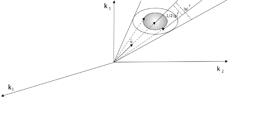
  Figure 2: The cone $\mathcal{C}_{\hat{u}}$ corresponding to the support of the smooth characteristic function $\xi_{\hat{u}}^{g}(\hat{k})$.

  We also define

  $$d_{n}^{\hat{u}}\,:=\,\frac{1}{2}\chi_{n}(|{\vec{k}}|)\xi_{\hat{u}}^{g}(\hat{k})[\,{\vec{k}}\cdot\,i{\vec{\nabla}}_{{\vec{k}}}+i{\vec{\nabla}}_{{\vec{k}}}\cdot\,{\vec{k}}\,]\chi_{n}(|{\vec{k}}|)\xi_{\hat{u}}^{g}(\hat{k})\,,$$ (III.18)

  and we introduce the second quantized operator

  $$D_{n}^{\hat{u}}\,:=\,d\Gamma(d_{n}^{\hat{u}})\,.$$ (III.19)

  Later on in the paper, when we implement the virial argument, we will make use of the creation/annihilation operators

  $$a^{*}(id_{n}^{\hat{u}}\rho_{\vec{x}})=\int d^{3}k\,i(d_{n}^{\hat{u}}\rho_{\vec{x}})({\vec{k}})a^{*}_{{\vec{k}}}$$

  $$a(id_{n}^{\hat{u}}\rho_{\vec{x}})=\int d^{3}k\,\overline{i(d_{n}^{\hat{u}}\rho_{\vec{x}})({\vec{k}})}a_{{\vec{k}}},$$

  and, analogously, $a(id_{n,\perp}^{\hat{u},\hat{Q}}\rho_{{\vec{x}}})$, $a^{*}(id_{n,\perp}^{\hat{u},\hat{Q}}\rho_{{\vec{x}}})$. In Lemma IV.1, we show that the vector $\Psi_{f_{\vec{Q}}^{g}}$ belongs to the form domain of these operators.

• Virial argument in each fiber space ${\mathcal{H}}_{{\vec{P}}}$.

  Here we consider

  $$D^{b}_{\frac{1}{\kappa},\kappa}\,:=\,d\Gamma^{b}(d_{\frac{1}{\kappa},\kappa})\,$$

  as the conjugate operator, where

  $$d_{\frac{1}{\kappa},\kappa}\,:=\,\chi_{[\frac{1}{\kappa},\kappa]}(|{\vec{k}}|)\frac{1}{2}\,({\vec{k}}\cdot\,i{\vec{\nabla}}_{{\vec{k}}}+i{\vec{\nabla}}_{{\vec{k}}}\cdot\,{\vec{k}})\chi_{[\frac{1}{\kappa},\kappa]}(|{\vec{k}}|)\,.$$ (III.20)

  $\chi_{[\frac{1}{\kappa},\kappa]}(|{\vec{k}}|)$, $\infty>\kappa>\max\{\Lambda,1\}$, are non-negative, $C^{\infty}(\mathbb{R}^{+})$ functions with the properties:

  • $\chi_{[\frac{1}{\kappa},\kappa]}(|{\vec{k}}|)=0$ for $|{\vec{k}}|\geq 2\kappa$, $|{\vec{k}}|\leq\frac{1}{2\kappa}$;

  • $\chi_{[\frac{1}{\kappa},\kappa]}(|{\vec{k}}|)=1$ for $\frac{1}{\kappa}\leq|{\vec{k}}|\leq\kappa$;

  • for some $C>0$, $|\chi^{\prime}_{[\frac{1}{\kappa},\kappa]}(|{\vec{k}}|)|<C\kappa$;

  Analogously to $a^{*}(id_{n}^{\hat{u}}\rho_{{\vec{x}}}),a(id_{n}^{\hat{u}}\rho_{{\vec{x}}})$, we will use

  $$b^{*}(id_{\frac{1}{\kappa},\kappa}\,\rho)=\int d^{3}k\,(id_{\frac{1}{\kappa},\kappa}\,\rho)({\vec{k}})b^{*}_{{\vec{k}}}$$

  $$b(id_{\frac{1}{\kappa},\kappa}\,\rho)=\int d^{3}k\,\overline{(id_{\frac{1}{\kappa},\kappa}\,\rho)({\vec{k}})}b_{{\vec{k}}}.$$

We will also consider the $g$-dependent cones (see Figure 3),

$$\mathcal{C}_{\hat{P}}^{a}:=\{{\vec{k}}\,\,:\,\,|\hat{k}\cdot\hat{P}|\leq\cos(a|g|^{\gamma/8})\}\,,$$ (III.21)

and use the smooth functions $\xi_{\mathcal{C}_{\hat{P}}^{a}}^{g}(\hat{k})$, $a=\frac{1}{2},2$, defined below.

The functions $\xi_{\mathcal{C}_{\hat{P}}^{a}}^{g}(\hat{k})$, $0\leq\xi_{\mathcal{C}_{\hat{P}}^{a}}^{g}(\hat{k})\leq 1$, are chosen such that

• $$\xi_{\mathcal{C}_{\hat{P}}^{a}}^{g}(\hat{k})=1\quad\text{for}\quad\{\hat{k}\,\,:\,\,|\hat{k}\cdot\hat{P}|\leq\cos(2a|g|^{\gamma/8})\}\,;$$ (III.22)

• $$\xi_{\mathcal{C}_{\hat{P}}^{a}}^{g}(\hat{k})=0\quad\text{for}\quad\{\hat{k}\,\,:\,\,|\hat{k}\cdot\hat{P}|>\cos(a|g|^{\gamma/8})\}\,;$$ (III.23)

• $$|\partial_{\theta_{\hat{kP}}}\xi_{\mathcal{C}_{\hat{P}}^{a}}^{g}(\hat{k})|\leq C_{\xi}\,|g|^{-\gamma/8}\,,$$ (III.24)

  for a constant $C_{\xi}$ independent of $g$, where $\theta_{\hat{kP}}$ is the angle between $\hat{k}$ and $\hat{P}$.

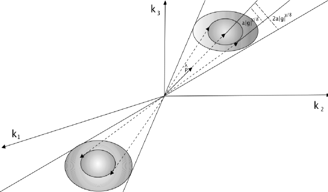
Figure 3: The double cone $\mathcal{C}_{\hat{P}}^{a}$ is the complement in $\mathbb{R}^{3}$ of the inner double cone around $\hat{P}$ of angular width $a|g|^{\gamma/8}$.

III.3 Description of strategy

To exclude the existence of eigenvalues $E_{{\vec{P}}}$, $|{\vec{P}}|>1$, we elaborate on an argument introduced in [12]. The idea of the proof is as follows. One assumes that an eigenvector $\Psi_{{\vec{P}},E_{{\vec{P}}}}\in{\mathcal{H}}_{{\vec{P}}}$ of $H_{{\vec{P}}}$ exists, for some energy $E_{{\vec{P}}}$ in a compact set. Then, using a multiscale virial argument, one intends to prove that

$$(\Psi_{{\vec{P}},E_{{\vec{P}}}},N^{b}\Psi_{{\vec{P}},E_{{\vec{P}}}})\leq{\mathcal{O}}(g^{2})\,,$$ (III.25)

where $N^{b}$ is the boson number operator in the fiber spaces. The multiscale virial argument involves the dilatation operators

$$d_{n}\,:=\,\frac{1}{2}\chi_{n}(|{\vec{k}}|)[\,{\vec{k}}\cdot\,i{\vec{\nabla}}_{{\vec{k}}}+i{\vec{\nabla}}_{{\vec{k}}}\cdot\,{\vec{k}}\,]\chi_{n}(|{\vec{k}}|)\,,$$ (III.26)

on the one-particle space $\mathfrak{h}$, where $\chi_{n}$ is a suitable smooth approximation to the characteristic function of the interval $[\frac{1}{n+1}\,,\,\frac{1}{n}]$ contained in the positive frequency half axis, $n=1,2,...$. After introducing the second quantized dilatation operators $D_{n}^{b}:=d\Gamma^{b}(d_{n})$, one starts from the formal virial identity

$$0=(\Psi_{{\vec{P}},E_{{\vec{P}}}}\,,\,i[H_{{\vec{P}}}\,,\,D_{n}^{b}]\,\Psi_{{\vec{P}},E_{{\vec{P}}}})$$ (III.27)

to establish the scale-by-scale inequality below, in a rigorous way:

$$(\Psi_{{\vec{P}},E_{{\vec{P}}}}\,,\,N^{b}_{n}\Psi_{{\vec{P}},E_{{\vec{P}}}})\leq{\mathcal{O}}(g^{2}n^{2}\||{\vec{k}}|^{\beta}\,{\bf 1}_{(\frac{1}{2(n+1)},\frac{3}{2n})}({\vec{k}})\|_{2}^{2})\,,$$ (III.28)

where $N^{b}_{n}:=\int\,d^{3}k\,a^{*}({\vec{k}})\chi_{n}^{2}(|{\vec{k}}|)a({\vec{k}})$, $n=1,2,3,\dots$. If (III.28) holds true, for sufficiently large values of the exponent $\beta$ in the form factor $\rho$, one can sum over $n$ and conclude that $(\Psi_{{\vec{P}},E_{{\vec{P}}}}\,,\,N^{b}\Psi_{{\vec{P}},E_{{\vec{P}}}})\leq{\mathcal{O}}(g^{2})$. Next, the eigenvalue equation (II.22) and the inequality in Eq. (III.25) can be combined to conclude that the vector $\Psi_{{\vec{P}},E_{{\vec{P}}}}$ and the eigenvalue $E_{{\vec{P}}}$ must fulfill the following estimates:

$$\|\Psi_{{\vec{P}},E_{{\vec{P}}}}-\Psi_{{\vec{P}}}^{0}\|^{2}\leq{\mathcal{O}}(g^{2})\,,$$ (III.29)

where $\Psi_{{\vec{P}}}^{0}:=\Omega_{f}$ is the unperturbed eigenstate, and

$$|E_{{\vec{P}}}-\frac{{\vec{P}}^{2}}{2}|\leq{\mathcal{O}}(g^{2})\,.$$ (III.30)

This result would imply that putative eigenvalues of $H_{{\vec{P}}}$ lie in an ${\mathcal{O}}(g^{2})$-neighborhood of the eigenvalue of the Hamiltonian $H^{g=0}_{{\vec{P}}}$.

Then the argument proceeds with the construction of suitable trial states of the type

$$\eta_{\vec{P}}\,:=\,\int\,d^{3}k\,\,\frac{1}{\epsilon^{\frac{1}{2}}}\,h\big{(}\frac{({\vec{P}}-{\vec{k}})^{2}/2+|{\vec{k}}|-E_{{\vec{P}}}}{\epsilon}\big{)}b^{*}_{{\vec{k}}}\,\Psi_{{\vec{P}}}^{0}\,,$$ (III.31)

where $\epsilon>0$ and $h(z)\in C_{0}^{\infty}(\mathbb{R})$, $h(z)\geq 0$. One then exploits the identity

$$(\eta_{\vec{P}}\,,\,(H_{{\vec{P}}}-E_{{\vec{P}}})\Psi_{{\vec{P}},E_{{\vec{P}}}})=0\,$$ (III.32)

that must hold true if $\Psi_{{\vec{P}},E_{{\vec{P}}}}$ is an eigenvector of $H_{{\vec{P}}}$. Starting from Eqs. (III.29)-(III.30), and using that the equation

$$({\vec{P}}-{\vec{k}})^{2}/2+|{\vec{k}}|-E_{{\vec{P}}}=0$$ (III.33)

has solutions for $|{\vec{P}}|>1$, provided $|g|$ is small enough, one arrives at a contradiction, for $\epsilon$ and $|g|$ small enough.

However, the procedure just outlined (mimicking the treatment of atomic resonances in [12]) will not work without some important modifications. We will therefore implement analogous, but more elaborate strategy.

The first problem ecountered is that we cannot control the expectation value

$$(\Psi_{{\vec{P}},E_{{\vec{P}}}},N^{b}\Psi_{{\vec{P}},E_{{\vec{P}}}})$$

by a multiscale virial argument in the fiber space ${\mathcal{H}}_{{\vec{P}}}$, because of the term $({\vec{P}}^{f})^{2}$ in $H_{{\vec{P}}}$. The commutator of $({\vec{P}}^{f})^{2}$ with $d\Gamma^{b}(d_{n})$, formally given by

$${\vec{P}}^{f}\cdot d\Gamma^{b}(\chi_{n}^{2}({\vec{k}}){\vec{k}})+d\Gamma^{b}(\chi_{n}^{2}({\vec{k}}){\vec{k}})\cdot{\vec{P}}^{f}\,,$$ (III.34)

cannot be controlled in terms of the commutator of $H^{f}$ with $d\Gamma^{b}(d_{n})$ . Consequently, the estimate in Eq. (III.28) cannot be justified starting from the virial identity in Eq. (III.27).

At the price of limiting our analysis to regular mass shells (see Main Theorem in Section II.4), this problem can be circumvented by implementing a multiscale virial argument in the full Hilbert space, by using single-particle “wave packets” rather than fiber eigenvectors, i.e., vectors in ${\mathcal{H}}$ of the type

$$\Psi_{f}\,:=\,\int f({\vec{P}})\,\Psi_{{\vec{P}},E_{{\vec{P}}}}d^{3}P\,,$$ (III.35)

where $f({\vec{P}})$ is a smooth function with support in $I_{g}$ (the region of momenta for which an eigenstate was assumed to exist). In practice, we choose $f=f_{\vec{Q}}^{g}$ to be sharply peaked around a given momentum $\vec{Q}$, see definition below (III.11). In the full Hilbert space, we can essentially mimick the treatement of atomic resonances to derive the following result (see Section IV).

Theorem (IV.3).

For $|g|$ sufficiently small,

$$\frac{(\Psi_{f_{\vec{Q}}^{g}}\,,\,N_{n,\mathcal{C}_{\hat{Q}}^{1/2}}\,\Psi_{f_{\vec{Q}}^{g}})}{(\Psi_{f_{\vec{Q}}^{g}}\,,\,\Psi_{f_{\vec{Q}}^{g}})}\leq\,{\mathcal{O}}(g^{2(1-2\gamma)}n^{2}\||{\vec{k}}|^{\beta}\,{\bf 1}_{(\frac{1}{2(n+1)},\frac{3}{2n})}({\vec{k}})\|_{2}^{2})\,,$$ (III.36)

where $N_{n,\mathcal{C}_{\hat{Q}}^{1/2}}:=d\Gamma(\chi_{n}^{2}(|{\vec{k}}|)\xi_{\mathcal{C}_{\hat{Q}}^{1/2}}^{g\,2}(\hat{k}))$ and $|\vec{Q}|\in I^{\prime}_{g}$.

Furthermore, if for all ${\vec{P}}\in suppf_{\vec{Q}}^{g}$ the inequality

$$||{\vec{\nabla}}E_{{\vec{P}}}|-1|>|g|^{\gamma/3}$$

holds true, then

$$\frac{(\Psi_{f_{\vec{Q}}^{g}}\,,\,N_{n}\,\Psi_{f_{\vec{Q}}^{g}})}{(\Psi_{f_{\vec{Q}}^{g}}\,,\,\Psi_{f_{\vec{Q}}^{g}})}\leq\,{\mathcal{O}}(g^{2(1-2\gamma)}n^{2}\||{\vec{k}}|^{\beta}\,{\bf 1}_{(\frac{1}{2(n+1)},\frac{3}{2n})}({\vec{k}})\|_{2}^{2})\,,$$ (III.37)

where $N_{n}:=d\Gamma(\chi_{n}^{2}(|{\vec{k}}|)$.

The constants in (III.36), (III.37) can be chosen uniformly in $\vec{Q}$, $|\vec{Q|}\in I^{\prime}_{g}\subset I$ ($I^{\prime}_{g}$ is defined in Section III.2, Eqs. (III.9),(III.10)). They only depend on $I$ and on $\Delta_{I}$.

By exploiting the $g$-dependence of the wavefunctions $f_{\vec{Q}}^{g}$ and the assumption on the regularity in ${\vec{P}}$ of $\Psi_{{\vec{P}},E_{{\vec{P}}}}$, one can convert a bound for the number operator $N$ on single-particle wave packets to a bound that holds pointwise in ${\vec{P}}$ on the number operator $N^{b}$ acting on the fiber eigenvectors $\Psi_{{\vec{P}},E_{{\vec{P}}}}$. In essence, this follows from the fundamental theorem of calculus. These arguments are implemented in Section IV and give the following results.

Theorem (IV.5).

For $|g|$ sufficiently small and $({\vec{P}},E_{{\vec{P}}})\in I^{\prime}_{g}\times\Delta_{I}$,

$$(\Psi_{{\vec{P}},E_{{\vec{P}}}}\,,\,N_{n,\mathcal{C}_{\hat{P}}^{2}}^{b}\,\Psi_{{\vec{P}},E_{{\vec{P}}}})\leq{\mathcal{O}}(|g|^{\frac{(1-2\gamma)}{3}}|g|^{-\gamma/8}n^{\frac{4}{3}}\,\||{\vec{k}}|^{\beta}\,{\bf 1}_{(\frac{1}{2(n+1)},\frac{3}{2n})}({\vec{k}})\|_{2}^{\frac{1}{3}})\,,$$ (III.38)

where

$$N_{n,\mathcal{C}_{\hat{P}}^{2}}^{b}:=d\Gamma^{b}(\chi_{n}^{2}(|{\vec{k}}|)\,\xi_{\mathcal{C}_{\hat{P}}^{2}}^{g\,2}(\hat{k}))\,.$$ (III.39)

Furthermore, if in addition $||{\vec{\nabla}}E_{\vec{P}}|-1|>\frac{3}{2}|g|^{\gamma/3}\,$ then

$$(\Psi_{{\vec{P}},E_{{\vec{P}}}}\,,\,N_{n}^{b}\,\Psi_{{\vec{P}},E_{{\vec{P}}}})\leq{\mathcal{O}}(|g|^{\frac{(1-2\gamma)}{3}}n^{\frac{4}{3}}\||{\vec{k}}|^{\beta}\,{\bf 1}_{(\frac{1}{2(n+1)},\frac{3}{2n})}({\vec{k}})\|_{2}^{\frac{1}{3}}))\,$$ (III.40)

where

$$N_{n}^{b}:=d\Gamma^{b}(\chi_{n}^{2}(|{\vec{k}}|))\,.$$ (III.41)

The constants in (III.38), (III.40) can be chosen uniformly in $\vec{P}$, $|\vec{P|}\in I^{\prime}_{g}\subset I$ ($I^{\prime}_{g}$ is defined in Section III.2, Eqs. (III.9), (III.10)). They only depend on $I$ and on $\Delta_{I}$.

We now comment on the contents of Theorem IV.5. Inequality (III.38) means that we can bound the boson number operator if we exclude a double cone (see Figure 3) and the definition of $\mathcal{C}_{\hat{P}}^{2}$ in Eqs. (III.22)-(III.24), Section III.2) around the direction of the particle velocity, provided the form factor $\rho({\vec{k}})$ scales like $|{\vec{k}}|^{\beta}$ with $\beta>{11/2}$, i.e.  (II.14).

The second result (see (III.40)) says that, for putative mass shells $({\vec{P}},E_{{\vec{P}}})$ such that $||{\vec{\nabla}}E_{\vec{P}}|-1|$ is not too small (i.e., $||{\vec{\nabla}}E_{\vec{P}}|-1|>\frac{3}{2}|g|^{\gamma/3}$), we can bound the boson number without any angular restrictions, again using that $\rho({\vec{k}})$ scales like $|{\vec{k}}|^{\beta}$ with $\beta>{11/2}$. The constraint means that the forward emission of bosons by the (massive) particle cannot be controlled if its speed is too close to the boson propagation speed.
The estimates on the number operator obtained in Section IV are used in Section V, where we will establish the following two results regarding the region $I_{g}\times\Delta_{I}$, where $I_{g}$ is any open interval contained in $I$ such that $|I_{g}|>|g|^{\gamma/2}$.

• The first result is that we can exclude all the regular mass shells except those with slope close to $1$, i.e., all the regular mass shells such that

  $$({\vec{P}},E_{{\vec{P}}})\in I_{g}\times\Delta_{I}\,\quad\text{and}\quad||{\vec{\nabla}}E_{\vec{P}}|-1|>\frac{3}{2}|g|^{\gamma/3}\,.$$ (III.42)

• The second result shows that a regular mass shell might exist only for $({\vec{P}},E_{{\vec{P}}})$ such that

  $$E_{{\vec{P}}}=|{\vec{P}}|-\frac{1}{2}+{\mathcal{O}}(|g|^{\gamma/4})\,.$$ (III.43)

More precisely, we use that:

• The expectation value in $\Psi_{{\vec{P}},E_{{\vec{P}}}}$, $|{\vec{P}}|\in I^{\prime}_{g}$, of the operator $N^{b}$ restricted to the angular sector $\mathcal{C}_{\hat{P}}^{2}$ vanishes as $g\to 0$ (see Theorem IV.5).

• For $({\vec{P}},E_{{\vec{P}}})\in I^{\prime}_{g}\times\Delta_{I}$ such that $||{\vec{\nabla}}E_{P}|-1|>{\mathcal{O}}(|g|^{\gamma/3})$, the expectation value of the number operators $N^{b}$ on $\Psi_{{\vec{P}},E_{{\vec{P}}}}$ vanishes as $g\to 0$; see Theorem IV.5. Analogously, if $suppf_{\vec{Q}}^{g}\subset\{({\vec{P}},E_{{\vec{P}}})\in I^{\prime}_{g}\times\Delta_{I}\,\,|\,\,||{\vec{\nabla}}E_{P}|-1|>{\mathcal{O}}(|g|^{\gamma/3})\}$ then the expectation value of the number operator $N$ on $\Psi_{f_{\vec{Q}}}^{g}$ vanishes as $g\to 0$; see Theorem IV.3.

• The results in (2) imply that the putative fiber eigenvectors $\Psi_{{\vec{P}},E_{{\vec{P}}}}$, $|{\vec{P}}|\in I^{\prime}_{g}$, and the corresponding energies $E_{{\vec{P}}}$ are pertubative in $g$ (see Corollary IV.6), provided that $\beta>{11/2}$.

We derive (i) in Theorem V.1 by mimicking the argument with the trial states employed for the treatment of the atomic resonances [12], which was anticipated in Section III.3, Eqs (III.31)–(III.33). To this end, we make us of (2) and (3).

The result in (ii) follows thanks to a stronger version of (1) (for details, see Lemma V.2, Lemma V.3) where only the forward cone around the direction of the particle velocity is excluded in the definition of the restricted number operator, and by combining the eigenvalue equation with a standard (i.e., not a multi-scale analysis) virial argument in the fiber space ${\mathcal{H}}_{{\vec{P}}}$, where the conjugate operator is $D_{\frac{1}{\kappa},\kappa}^{b}\,:=\,d\Gamma^{b}(d_{\frac{1}{\kappa},\kappa})$; see (III.20) and Theorem V.4.

The virial identity exploited in Theorem V.4 is actually enough to exclude that, fiber by fiber, the eigenvalue lies at a distance larger than ${\mathcal{O}}(g)$ above the unperturbed eigenvalue. This observation is explained in the Remark after Theorem V.4 in Section V. However, the instability of the unperturbed mass shell proven in this paper requires a detailed analysis of the configuration of bosons in the putative eigenvector whose momenta are contained in different cones of momentum space. The decay mechanism exploited in Theorem V.1 combined with the assumed continuity of the mass shell is responsible for the absence of single-particle states except for the region $E_{{\vec{P}}}=|{\vec{P}}|-\frac{1}{2}+{\mathcal{O}}(|g|^{\gamma/4})$. This is because if the particle propagated at the critical velocity, i.e., $|{\vec{\nabla}}E_{P}|=1$, then there would be no kinematical constraint preventing the emission of an arbitrarily large number of soft bosons in the forward direction (the direction of ${\vec{P}}$).

IV Boson number estimates

The main results in this section are Theorem IV.3, Theorem IV.5, and Corollary IV.6. Two preparatory results, contained in Section IV.1, are needed. In particular, in Lemma IV.2, we provide a rigorous justification of a virial identity employed in Lemma IV.4 and in Theorem IV.3.

Since the proof of Theorem IV.3 is lengthy, we present it in two different smaller sections: (a) In Section IV.2.1, we outline the proof of the theorem and, in Lemma IV.4, we introduce an important ingredient used later on. (b) In Section IV.2.2, we complete the steps of the proof by assuming the result obtained in Lemma IV.4.

In Section IV.3, by using the regularity properties that follow from the Main Hypothesis, we derive some estimates for the number operator $N^{b}$ evaluated on the fiber eigenvectors $\Psi_{{\vec{P}},E_{{\vec{P}}}}$ analogous to those obtained in Theorem IV.3 for the number operator $N$ evaluated on the single-particle states $\Psi_{f^{g}_{\vec{Q}}}$. In Corollary IV.6, we then finally show that $E_{{\vec{P}}}$ and $\Psi_{{\vec{P}},E_{{\vec{P}}}}$ are perturbative in $g$, provided $|{\vec{P}}|\in I^{\prime}_{g}$, $E_{{\vec{P}}}\in\Delta_{I}$, $\beta>{11/2}$, and $||{\vec{\nabla}}E_{{\vec{P}}}|-1|>\frac{3}{2}|g|^{\gamma/3}$.

IV.1 Preparatory results on virial identities

The following two lemmas are repeated and proven in Sections VI.1 and VI.2 of the appendix, respectively.

Lemma IV.1.

The vector $\Psi_{f_{\vec{Q}}^{g}}$ belongs to the domain of the position operator ${\vec{x}}$ and

$$\|x_{j}\Psi_{f_{\vec{Q}}^{g}}\|\leq{\mathcal{O}}(|g|^{-\gamma}\|\Psi_{f_{\vec{Q}}^{g}}\|),\qquad j=1,2,3\,.$$ (IV.1)

Proof.

See the appendix ∎

Lemma IV.2 states a virial theorem for our model. We observe that by formal steps one can derive the identity

$$\,i[H-E_{{\vec{P}}}\,,\,D_{n}^{\hat{u}}] = \,d\Gamma(i[|{\vec{k}}|,\,d_{n}^{\hat{u}}])-\,{\vec{\nabla}}E_{{\vec{P}}}\cdot d\Gamma(i[{\vec{k}},\,d_{n}^{\hat{u}}])$$

$$-g\,[a^{*}(id_{n}^{\hat{u}}\rho_{{\vec{x}}})+\,a(id_{n}^{\hat{u}}\rho_{{\vec{x}}})]\,,$$

where $E_{{\vec{P}}}$, and ${\vec{\nabla}}E_{{\vec{P}}}$ are operator-valued functions of the total momentum operator ${\vec{P}}$. Another formal step would imply that

$$0=(\Psi_{f_{\vec{Q}}^{g}}\,,\,i[H-E_{{\vec{P}}}\,,\,D_{n}^{\hat{u}}]\,\Psi_{f_{\vec{Q}}^{g}})\,,$$ (IV.3)

and, hence,

$$0 = (\Psi_{f_{\vec{Q}}^{g}}\,,\,d\Gamma(i[|{\vec{k}}|,\,d_{n}^{\hat{u}}])\Psi_{f_{\vec{Q}}^{g}})-(\Psi_{f_{\vec{Q}}^{g}}\,,\,{\vec{\nabla}}E_{{\vec{P}}}\cdot d\Gamma(i[{\vec{k}},\,d_{n}^{\hat{u}}])\Psi_{f_{\vec{Q}}^{g}})$$ (IV.4)

$$-g(\Psi_{f_{\vec{Q}}^{g}}\,,\,[a^{*}(id_{n}^{\hat{u}}\rho_{{\vec{x}}})+\,a(id_{n}^{\hat{u}}\rho_{{\vec{x}}})]\Psi_{f_{\vec{Q}}^{g}})\,.$$

The next Lemma shows that all terms on the RHS of Eq. (IV.4) can be given a well-defined meaning such that the equality is true.

Lemma IV.2.

The identity

$$0 = (\Psi_{f_{\vec{Q}}^{g}}\,,\,d\Gamma(\chi_{n}^{2}(|{\vec{k}}|)\xi^{g\,2}_{\hat{u}}(\hat{k})\,|{\vec{k}}|)\Psi_{f_{\vec{Q}}^{g}})-(\Psi_{f_{\vec{Q}}^{g}}\,,\,{\vec{\nabla}}E_{{\vec{P}}}\cdot d\Gamma(\chi_{n}^{2}(|{\vec{k}}|)\xi^{g\,2}_{\hat{u}}(\hat{k})\,{\vec{k}})\Psi_{f_{\vec{Q}}^{g}})$$ (IV.5)

$$-g(\Psi_{f_{\vec{Q}}^{g}}\,,\,[a^{*}(id_{n}^{\hat{u}}\rho_{{\vec{x}}})+\,a(id_{n}^{\hat{u}}\rho_{{\vec{x}}})]\Psi_{f_{\vec{Q}}^{g}})\,$$

holds true. As the one-particle state $\Psi_{f_{\vec{Q}}^{g}}$ belongs to the form domain of all operators on the RHS of $\eqref{eq:III.11}$, this RHS is well-defined.

Proof.

See the appendix ∎

Note that the formal equality of the RHS of (IV.4) and (IV.5) is straightforward. The virial identity of the Lemma above is first used in item (i) of IV.2.1. A similar virial identity in item (ii) is proven analogously.

IV.2 Number operator estimates in putative single-particle states

We now proceed to proving the following theorem, where the expectation of the boson number operator in the state $\Psi_{f_{\vec{Q}}^{g}}$ is bounded scale by scale.

Theorem IV.3.

For $|g|$ sufficiently small,

$$\frac{(\Psi_{f_{\vec{Q}}^{g}}\,,\,N_{n,\mathcal{C}_{\hat{Q}}^{1/2}}\,\Psi_{f_{\vec{Q}}^{g}})}{(\Psi_{f_{\vec{Q}}^{g}}\,,\,\Psi_{f_{\vec{Q}}^{g}})}\leq\,{\mathcal{O}}(|g|^{2(1-2\gamma)}n^{2}\||{\vec{k}}|^{\beta}\,{\bf 1}_{(\frac{1}{2(n+1)},\frac{3}{2n})}({\vec{k}})\|_{2}^{2})\,,$$ (IV.6)

where $N_{n,\mathcal{C}_{\hat{Q}}^{1/2}}:=d\Gamma(\chi_{n}^{2}(|{\vec{k}}|)\xi_{\mathcal{C}_{\hat{Q}}^{1/2}}^{g\,2}(\hat{k}))$ and $\vec{Q}\in I^{\prime}_{g}$.

Furthermore, if for all ${\vec{P}}\in suppf_{\vec{Q}}^{g}$ the inequality

$$||{\vec{\nabla}}E_{{\vec{P}}}|-1|>|g|^{\gamma/3}$$

holds true then

$$\frac{(\Psi_{f_{\vec{Q}}^{g}}\,,\,N_{n}\,\Psi_{f_{\vec{Q}}^{g}})}{(\Psi_{f_{\vec{Q}}^{g}}\,,\,\Psi_{f_{\vec{Q}}^{g}})}\leq\,{\mathcal{O}}(|g|^{2(1-2\gamma)}n^{2}\||{\vec{k}}|^{\beta}\,{\bf 1}_{(\frac{1}{2(n+1)},\frac{3}{2n})}({\vec{k}})\|_{2}^{2})\,,$$ (IV.7)

where $N_{n}:=d\Gamma(\chi_{n}^{2}(|{\vec{k}}|)$.

The (implicit) constants in (IV.6)-(IV.7) can be chosen to be uniform in $\vec{Q}$, $|\vec{Q|}\in I^{\prime}_{g}\subset I$; for the definition of $I^{\prime}_{g}$ see Eqs. (III.9), (III.10)). They only depend on $I$ and on $\Delta_{I}$.

IV.2.1 Outline of the proof of Theorem IV.3

To prove inequalities (IV.6), (IV.7) we exploit two different virial arguments and properties (P1), (P2), and (P3) of Sect. III.1.2. More precisely, we employ both conjugate operators $D_{n}^{\hat{u}}\,:=\,d\Gamma(d_{n}^{\hat{u}})$ and $D_{n,\perp}^{\hat{u},\hat{Q}}\,:=\,d\Gamma(d_{n,\perp}^{\hat{u},\hat{Q}})$, with $d_{n}^{\hat{u}}$ and $d_{n,\perp}^{\hat{u},\hat{Q}}$ defined in Eqs. (III.18) and (III.13), respectively. The virial identities (see Lemma IV.2 for a rigorous treatment of the identities below) corresponding to $D_{n}^{\hat{u}}$ and $D_{n,\perp}^{\hat{u},\hat{Q}}$ are:

• $$0 = (\Psi_{f_{\vec{Q}}^{g}}\,,\,d\Gamma(i[|{\vec{k}}|,\,d_{n}^{\hat{u}}])\Psi_{f_{\vec{Q}}^{g}})$$ (IV.10)

  $$-(\Psi_{f_{\vec{Q}}^{g}}\,,\,{\vec{\nabla}}E_{{\vec{P}}}\cdot d\Gamma(i[{\vec{k}},\,d_{n}^{\hat{u}}])\Psi_{f_{\vec{Q}}^{g}})$$

  $$-g(\Psi_{f_{\vec{Q}}^{g}}\,,\,[a^{*}(id_{n}^{\hat{u}}\rho_{{\vec{x}}})+\,a(id_{n}^{\hat{u}}\rho_{{\vec{x}}})]\Psi_{f_{\vec{Q}}^{g}})\,$$

  $$= (\Psi_{f_{\vec{Q}}^{g}}\,,\,d\Gamma(\chi_{n}^{2}(|{\vec{k}}|)\xi^{g\,2}_{\hat{u}}(\hat{k})\,|{\vec{k}}|)\Psi_{f_{\vec{Q}}^{g}})$$ (IV.13)

  $$-(\Psi_{f_{\vec{Q}}^{g}}\,,\,{\vec{\nabla}}E_{{\vec{P}}}\cdot d\Gamma(\chi_{n}^{2}(|{\vec{k}}|)\xi^{g\,2}_{\hat{u}}(\hat{k})\,{\vec{k}})\Psi_{f_{\vec{Q}}^{g}})$$

  $$-g(\Psi_{f_{\vec{Q}}^{g}}\,,\,[a^{*}(id_{n}^{\hat{u}}\rho_{{\vec{x}}})+\,a(id_{n}^{\hat{u}}\rho_{{\vec{x}}})]\Psi_{f_{\vec{Q}}^{g}})\,;$$

• $$0 = (\Psi_{f_{\vec{Q}}^{g}}\,,\,d\Gamma(i[|{\vec{k}}|,\,d_{n,\perp}^{\hat{u},\hat{Q}}])\Psi_{f_{\vec{Q}}^{g}})$$ (IV.16)

  $$-(\Psi_{f_{\vec{Q}}^{g}}\,,\,{\vec{\nabla}}E_{{\vec{P}}}\cdot d\Gamma(i[{\vec{k}},\,d_{n,\perp}^{\hat{u},\hat{Q}}])\Psi_{f_{\vec{Q}}^{g}})$$

  $$-g(\Psi_{f_{\vec{Q}}^{g}}\,,\,[a^{*}(id_{n,\perp}^{\hat{u},\hat{Q}}\rho_{{\vec{x}}})+\,a(id_{n,\perp}^{\hat{u},\hat{Q}}\rho_{{\vec{x}}})]\Psi_{f_{\vec{Q}}^{g}})$$

  $$= (\Psi_{f_{\vec{Q}}^{g}}\,,\,d\Gamma(\chi_{n}^{2}(|{\vec{k}}|)\xi^{g\,2}_{\hat{u}}(\hat{k})\,\frac{|{\vec{k}}_{\perp}|^{2}}{|{\vec{k}}|})\Psi_{f_{\vec{Q}}^{g}})$$ (IV.19)

  $$-(\Psi_{f_{\vec{Q}}^{g}}\,,\,{\vec{\nabla}}E_{{\vec{P}}}\cdot d\Gamma(\chi_{n}^{2}(|{\vec{k}}|)\xi^{g\,2}_{\hat{u}}(\hat{k})\,{\vec{k}}_{\perp})\Psi_{f_{\vec{Q}}^{g}})$$

  $$-g(\Psi_{f_{\vec{Q}}^{g}}\,,\,[a^{*}(id_{n,\perp}^{\hat{u},\hat{Q}}\rho_{{\vec{x}}})+\,a(id_{n,\perp}^{\hat{u},\hat{Q}}\rho_{{\vec{x}}})]\Psi_{f_{\vec{Q}}^{g}})\,.$$

(For the definition of the functions $\chi_{n}(|{\vec{k}}|)$, $\xi^{g}_{\hat{u}}(\hat{k})$ see (a) and (b), in Section III.2)

Next, we explain in detail the key role of the virial identities. In order to arrive at inequalities (IV.6), (IV.7), we study (see Lemma IV.4) the number operator restricted to the sector associated with the unit vector $\hat{u}$, and derive the estimate

$$(\Psi_{f_{\vec{Q}}^{g}}\,,\,N_{n,\hat{u}}\,\Psi_{f_{\vec{Q}}^{g}})\leq(\Psi_{f_{\vec{Q}}^{g}}\,,\,\Psi_{f_{\vec{Q}}^{g}})\,{\mathcal{O}}(|g|^{2(1-\gamma-\tilde{\gamma})}n^{2}\||{\vec{k}}|^{\beta}\,{\bf 1}_{(\frac{1}{2(n+1)},\frac{3}{2n})}({\vec{k}})\|_{2}^{2})\,,$$ (IV.20)

where $N_{n,\hat{u}}:=d\Gamma(\chi_{n}^{2}(|{\vec{k}}|)\xi_{\hat{u}}^{g\,2}(\hat{k}))$, for some $\tilde{\gamma}$, $0<\tilde{\gamma}<\gamma$; we will eventually choose $\tilde{\gamma}=\gamma/2$. In doing this, we start from the bound

$$|(\Psi_{f_{\vec{Q}}^{g}}\,,\,d\Gamma(\chi_{n}^{2}(|{\vec{k}}|)\xi^{g\,2}_{\hat{u}}(\hat{k})\,|{\vec{k}}|)\Psi_{f_{\vec{Q}}^{g}})-(\Psi_{f_{\vec{Q}}^{g}}\,,\,{\vec{\nabla}}E_{{\vec{P}}}\cdot d\Gamma(\chi_{n}^{2}(|{\vec{k}}|)\xi^{g\,2}_{\hat{u}}(\hat{k})\,{\vec{k}})\Psi_{f_{\vec{Q}}^{g}})|$$

$$\qquad\geq{\mathcal{O}}(|g|^{\tilde{\gamma}})(\Psi_{f_{\vec{Q}}^{g}}\,,\,d\Gamma(\chi_{n}^{2}(|{\vec{k}}|)\xi^{g\,2}_{\hat{u}}(\hat{k})\,|{\vec{k}}|)\Psi_{f_{\vec{Q}}^{g}})\quad\quad\quad\quad\quad\quad\quad\quad\quad$$ (IV.21)

that holds if, for all ${\vec{P}}\in suppf_{\vec{Q}}^{g}$ and for all $\hat{k}$ in the sector,

$$|1-\hat{k}\cdot{\vec{\nabla}}E_{{\vec{P}}}|>|g|^{\tilde{\gamma}}>0\,.$$ (IV.22)

Given (IV.2.1), it is straightfoward to control the term (see (IV.13)) associated with the interaction part of the Hamiltonian, and to derive the inequality in (IV.20). Therefore, the bound in (IV.22) is crucial, and we must identify the sectors where it is violated. We recall that ${\vec{\nabla}}E_{{\vec{P}}}$ is collinear to ${\vec{P}}$, and we may assume that they are parallel; the other case can be treated in the same way.

First, note that the angle between ${\vec{P}}\in suppf_{\vec{Q}}^{g}$ and $\vec{Q}$, as well as the angle between $\hat{u}$ and a vector ${\vec{k}}$ that belongs to the sector associated with $\hat{u}$, are ${\mathcal{O}}(|g|^{\gamma})$. This follows from the definitions of the function $f_{\vec{Q}}^{g}$ and the cones $\mathcal{C}_{\hat{u}}$, given in Section III.2. It implies that, roughly speaking, we can identify $\hat{P}=\hat{Q}$ and $\hat{k}=\hat{u}$, since, for $|g|$ small enough, $|g|^{\gamma}$ is much smaller than $|g|^{\tilde{\gamma}}$ in (IV.22).
The vectors ${\vec{k}}$ for which (IV.22) fails, satisfy

$$\left|\hat{k}\cdot\hat{P}-|{\vec{\nabla}}E_{{\vec{P}}}|^{-1}\right|\leq{\mathcal{O}}(|g|^{\tilde{\gamma}(=\gamma/2)}),\,\qquad|{\vec{\nabla}}E_{{\vec{P}}}|>0\,.$$ (IV.23)

Hence, if $|{\vec{\nabla}}E_{{\vec{P}}}|$ is bounded away from $1$, either - for $|{\vec{\nabla}}E_{{\vec{P}}}|<1$; see also (B) in Section IV.2.2 - the condition (IV.22) is always satisfied, or - for $|{\vec{\nabla}}E_{{\vec{P}}}|>1$; see also (C) in Section IV.2.2 - such ${\vec{k}}$ have a nonvanishing component, ${\vec{k}}_{\perp}$, (of order $\sqrt{1-|{\vec{\nabla}}E_{{\vec{P}}}|^{-2}}$) in the orthogonal complement of $\vec{Q}(=\vec{P})$. In particular, they satisfy

$$\big{|}\frac{|{\vec{k}}_{\perp}|^{2}}{|{\vec{k}}|^{2}}-\frac{|{\vec{k}}_{\perp}|}{|{\vec{k}}|}\hat{k}_{\perp}\cdot{\vec{\nabla}}E_{{\vec{P}}}\big{|}>{\mathcal{O}}(|g|^{\gamma/3})>0\,,$$ (IV.24)

Note that the second term on the LHS of (IV.24) actually vanishes if our approximation $\hat{P}=\hat{Q}$ were to hold exactly. In Section IV.2.2, we establish (IV.24) rigorously. The bound (IV.24) immediately implies that, for the sectors $\hat{u}$ for which (IV.22) fails, the following bound holds true

$$|(\Psi_{f_{\vec{Q}}^{g}}\,,\,d\Gamma(\chi_{n}^{2}(|{\vec{k}}|)\xi^{g\,2}_{\hat{u}}(\hat{k})\,\frac{|{\vec{k}}_{\perp}|^{2}}{|{\vec{k}}|})\Psi_{f_{\vec{Q}}^{g}})$$ (IV.25)

$$\,\,-(\Psi_{f_{\vec{Q}}^{g}}\,,\,{\vec{\nabla}}E_{{\vec{P}}}\cdot d\Gamma(\chi_{n}^{2}(|{\vec{k}}|)\xi^{g\,2}_{\hat{u}}(\hat{k})\,{\vec{k}}_{\perp})\Psi_{f_{\vec{Q}}^{g}})|$$

$$\geq {\mathcal{O}}(|g|^{\gamma/3})(\Psi_{f_{\vec{Q}}^{g}}\,,\,d\Gamma(\chi_{n}^{2}(|{\vec{k}}|)\xi^{g\,2}_{\hat{u}}(\hat{k})\,|{\vec{k}}|)\Psi_{f_{\vec{Q}}^{g}})\,,$$

Starting from this bound, we can use the second virial identity (IV.19, IV.19, IV.19) to derive the inequality (IV.20) for the sectors $\hat{u}$ for which (IV.22) fails.

The conclusion is that, under the condition that $|{\vec{\nabla}}E_{{\vec{P}}}|$, ${\vec{P}}\in suppf_{\vec{Q}}^{g}$, differs from $1$ by a quantity $>{\mathcal{O}}(|g|^{\gamma/3})$, we can cover all the sectors by the two virial identities above. Without the restriction on $|{\vec{\nabla}}E_{{\vec{P}}}|$, these arguments only show that Eq. (IV.20) holds for all $\hat{u}$-dependent sectors contained in the cone $\mathcal{C}^{1/2}_{\hat{Q}}$.

In implementing this strategy, we make use of the following lemma.

Lemma IV.4.

Fix a unit vector $\hat{u}$ and assume that, for all ${\vec{P}}\in suppf_{\vec{Q}}^{g}$ and for all $\hat{k}\in supp\,\xi_{\hat{u}}^{g}$,

$$|1-\hat{k}\cdot{\vec{\nabla}}E_{{\vec{P}}}|>|g|^{\tilde{\gamma}}>0\,,\quad\quad 0<\tilde{\gamma}<\gamma\,,$$ (IV.26)

where $\tilde{\gamma}$ is $g$- and $\vec{Q}$-independent. Then, for $|g|$ small enough, the following bound holds true

$$(\Psi_{f_{\vec{Q}}^{g}}\,,\,N_{n,\hat{u}}\,\Psi_{f_{\vec{Q}}^{g}})\leq(\Psi_{f_{\vec{Q}}^{g}}\,,\,\Psi_{f_{\vec{Q}}^{g}})\,{\mathcal{O}}(|g|^{2(1-\gamma-\tilde{\gamma})}n^{2}\||{\vec{k}}|^{\beta}\,{\bf 1}_{(\frac{1}{2(n+1)},\frac{3}{2n})}({\vec{k}})\|_{2}^{2})\,,$$ (IV.27)

where $N_{n,\hat{u}}:=d\Gamma(\chi_{n}^{2}(|{\vec{k}}|)\xi_{\hat{u}}^{g\,2}(\hat{k}))$.

Proof

We assume that (IV.26) holds with

$$1-\hat{k}\cdot{\vec{\nabla}}E_{{\vec{P}}}<0;$$

the other case, $1-\hat{k}\cdot{\vec{\nabla}}E_{{\vec{P}}}>0$, can be treated similarly. We get

$$0 = (\Psi_{f_{\vec{Q}}^{g}}\,,\,d\Gamma(\chi_{n}^{2}(|{\vec{k}}|)\xi_{\hat{u}}^{g\,2}(\hat{k})\,|{\vec{k}}|)\Psi_{f_{\vec{Q}}^{g}})\quad\,\,$$

$$-(\Psi_{f_{\vec{Q}}^{g}}\,,\,{\vec{\nabla}}E_{{\vec{P}}}\cdot d\Gamma(\chi_{n}^{2}(|{\vec{k}}|)\xi_{\hat{u}}^{g\,2}(\hat{k})\,{\vec{k}})\Psi_{f_{\vec{Q}}^{g}})\quad\quad\quad\,\,$$

$$-g(\Psi_{f_{\vec{Q}}^{g}}\,,\,[a^{*}(id_{n}^{\hat{u}}\rho_{{\vec{x}}})+\,a(id_{n}^{\hat{u}}\rho_{{\vec{x}}})]\Psi_{f_{\vec{Q}}^{g}})\,$$

$$\leq -|g|^{\tilde{\gamma}}(\Psi_{f_{\vec{Q}}^{g}}\,,\,d\Gamma(\chi_{n}^{2}(|{\vec{k}}|)\xi_{\hat{u}}^{g\,2}(\hat{k})|{\vec{k}}|)\Psi_{f_{\vec{Q}}^{g}})$$

$$+c|g|^{1-\gamma}\|\Psi_{f_{\vec{Q}}^{g}}\|\|d\Gamma(\chi_{n}^{2}(|{\vec{k}}|)\xi_{\hat{u}}^{g\,2}(\hat{k}))^{1/2}\Psi_{f_{\vec{Q}}^{g}}\|\times$$

$$\quad\times(\int|{\vec{k}}|^{2\beta}\,{\bf 1}_{(\frac{1}{2(n+1)},\frac{3}{2n})}({\vec{k}})\,d^{3}k)^{1/2}$$

for some constant $c$, $c>0$, uniform in $\vec{Q}$, $|\vec{Q}|\in I^{\prime}_{g}$. To do the step from (IV.2.1) to (IV.2.1), we split

$$i(d_{n}^{\hat{u}}\rho_{{\vec{x}}})({\vec{k}}) = -\,\chi_{n}(|{\vec{k}}|)\,\xi_{\hat{u}}^{g}(\hat{k})\,\big{(}{\vec{k}}\cdot{\vec{\nabla}}_{{\vec{k}}}\big{(}\chi_{n}(|{\vec{k}}|)\xi_{\hat{u}}^{g}(\hat{k})\big{)}\big{)}\,{\rho}({\vec{k}})\,e^{-i{\vec{k}}\cdot{\vec{x}}}\,\quad\quad\quad$$ (IV.31)

$$-\,\chi_{n}^{2}(|{\vec{k}}|)\xi_{\hat{u}}^{g\,2}(\hat{k})\,\big{(}{\vec{k}}\cdot{\vec{\nabla}}_{{\vec{k}}}{\rho}({\vec{k}})\big{)}e^{-i{\vec{k}}\cdot{\vec{x}}}$$

$$-\frac{1}{2}\,\chi_{n}^{2}(|{\vec{k}}|)\xi_{\hat{u}}^{g\,2}(\hat{k})\,\big{(}{\vec{\nabla}}_{{\vec{k}}}\cdot{\vec{k}}\big{)}\,{\rho}({\vec{k}})\;e^{-i{\vec{k}}\cdot{\vec{x}}}$$

$$-\,\chi_{n}^{2}(|{\vec{k}}|)\xi_{\hat{u}}^{g\,2}(\hat{k})\,{\rho}({\vec{k}})\,\big{(}{\vec{k}}\cdot{\vec{\nabla}}_{{\vec{k}}}e^{-i{\vec{k}}\cdot{\vec{x}}}\big{)}\,$$

and we may justify this step for each of the four terms separately, using the Schwarz inequality and

• The assumption $\left|1-\hat{k}\cdot{\vec{\nabla}}E_{{\vec{P}}}\right|>|g|^{\tilde{\gamma}}$ for ${\vec{P}}\in suppf_{\vec{Q}}^{g}$;

• The infrared behavior of $\rho({\vec{k}})$ as assumed in (II.14), i.e., $|\rho({\vec{k}})|\leq{\mathcal{O}}(|{\vec{k}}|^{\beta})$ and $|{\vec{\nabla}}_{{\vec{k}}}{\rho}({\vec{k}})|\leq{\mathcal{O}}(|{\vec{k}}|^{\beta-1})$;

• Lemma IV.1.

As an example, for the term proportional to

$$-\,\chi_{n}^{2}(|{\vec{k}}|)\xi_{\hat{u}}^{g\,2}(\hat{k})\,{\rho}({\vec{k}})\,\big{(}{\vec{k}}\cdot{\vec{\nabla}}_{{\vec{k}}}e^{-i{\vec{k}}\cdot{\vec{x}}}\big{)}$$

we proceed as follows:

$$\left|(\Psi_{f_{\vec{Q}}^{g}}\,,\,a^{*}\big{(}-\,\chi_{n}^{2}(|{\vec{k}}|)\xi_{\hat{u}}^{g\,2}(\hat{k})\,\rho({\vec{k}})\,\big{(}{\vec{k}}\cdot{\vec{\nabla}}_{{\vec{k}}}e^{-i{\vec{k}}\cdot{\vec{x}}}\big{)}\big{)}\Psi_{f_{\vec{Q}}^{g}})\right|$$ (IV.32)

$$= \left|\int\,\chi_{n}^{2}(|{\vec{k}}|)\xi_{\hat{u}}^{g\,2}(\hat{k})\,\rho({\vec{k}})\,{\vec{k}}\cdot(a_{{\vec{k}}}\Psi_{f_{\vec{Q}}^{g}}\,,\,{\vec{\nabla}}_{{\vec{k}}}e^{-i{\vec{k}}\cdot{\vec{x}}}\Psi_{f_{\vec{Q}}^{g}})d^{3}k\right|$$

$$\leq \int\,\chi_{n}^{2}(|{\vec{k}}|)\xi_{\hat{u}}^{g\,2}(\hat{k})\,|\rho({\vec{k}})|\,|{\vec{k}}|\,|(a_{{\vec{k}}}\Psi_{f_{\vec{Q}}^{g}}\,,\,{\vec{\nabla}}_{{\vec{k}}}e^{-i{\vec{k}}\cdot{\vec{x}}}\Psi_{f_{\vec{Q}}^{g}})|d^{3}k$$

$$\leq \int\,\chi_{n}^{2}(|{\vec{k}}|)\xi_{\hat{u}}^{g\,2}(\hat{k})\,|\rho({\vec{k}})|\,|{\vec{k}}|\,\|a_{{\vec{k}}}\Psi_{f_{\vec{Q}}^{g}}\|\|{\vec{\nabla}}_{{\vec{k}}}e^{-i{\vec{k}}\cdot{\vec{x}}}\Psi_{f_{\vec{Q}}^{g}}\|d^{3}k$$

$$\leq \big{(}\int\,\chi_{n}^{2}(|{\vec{k}}|)\xi_{\hat{u}}^{g\,2}(\hat{k})\,\|a_{{\vec{k}}}\Psi_{f_{\vec{Q}}^{g}}\|^{2}d^{3}k\big{)}^{1/2}\times$$

$$\times\big{(}\int\|{\vec{\nabla}}_{{\vec{k}}}e^{-i{\vec{k}}\cdot{\vec{x}}}\Psi_{f_{\vec{Q}}^{g}}\|^{2}\,|{\vec{k}}|^{2\beta}\,{\bf 1}_{(\frac{1}{2(n+1)},\frac{3}{2n})}({\vec{k}})\,|{\vec{k}}|^{2}d^{3}k\big{)}^{1/2}\,.$$

We notice that

$$\big{(}\int\,\chi_{n}^{2}(|{\vec{k}}|)\xi_{\hat{u}}^{g\,2}(\hat{k})\,\|a_{{\vec{k}}}\Psi_{f_{\vec{Q}}^{g}}\|^{2}d^{3}k\big{)}^{1/2}=\|d\Gamma(\chi_{n}^{2}(|{\vec{k}}|)\xi_{\hat{u}}^{g\,2}(\hat{k}))^{1/2}\Psi_{f_{\vec{Q}}^{g}}\|$$ (IV.33)

and, since $\|{\vec{\nabla}}_{{\vec{k}}}e^{-i{\vec{k}}\cdot{\vec{x}}}\Psi_{f_{\vec{Q}}^{g}}\|\leq{\mathcal{O}}(|g|^{-\gamma}\|\Psi_{f_{\vec{Q}}^{g}}\|)$ (Lemma IV.1),

$$\big{(}\int\|{\vec{\nabla}}_{{\vec{k}}}e^{-i{\vec{k}}\cdot{\vec{x}}}\Psi_{f_{\vec{Q}}^{g}}\|^{2}|{\vec{k}}|^{2\beta}\,{\bf 1}_{(\frac{1}{2(n+1)},\frac{3}{2n})}({\vec{k}})\,|{\vec{k}}|^{2}d^{3}k\big{)}^{1/2}$$ (IV.34)

$$\leq C|g|^{-\gamma}(\int|{\vec{k}}|^{2\beta}\,{\bf 1}_{(\frac{1}{2(n+1)},\frac{3}{2n})}({\vec{k}})\,d^{3}k)^{1/2}\|\Psi_{f_{\vec{Q}}^{g}}\|\,.$$ (IV.35)

Then, starting from (IV.2.1), the bound from above takes the form

$$(\Psi_{f_{\vec{Q}}^{g}}\,,\,N_{n,\hat{u}}\,\Psi_{f_{\vec{Q}}^{g}})\leq(\Psi_{f_{\vec{Q}}^{g}}\,,\,\Psi_{f_{\vec{Q}}^{g}})\,{\mathcal{O}}(|g|^{2(1-\gamma-\tilde{\gamma})}n^{2}\||{\vec{k}}|^{\beta}\,{\bf 1}_{(\frac{1}{2(n+1)},\frac{3}{2n})}({\vec{k}})\|_{2}^{2})\,,$$ (IV.36)

where $N_{n,\hat{u}}:=d\Gamma(\chi_{n}^{2}(|{\vec{k}}|)\xi_{\hat{u}}^{g\,2}(\hat{k}))$, because

$$\chi_{n}^{2}(|{\vec{k}}|)\xi_{\hat{u}}^{g\,2}(\hat{k})|{\vec{k}}|\geq\frac{1}{2(n+1)}\chi_{n}^{2}(|{\vec{k}}|)\xi_{\hat{u}}^{g\,2}(\hat{k})\,.$$ (IV.37)

blablabla ∎

IV.2.2 Proof of Theorem IV.3

Notice that, starting from Lemma IV.4, we can fill the region

$$\{\hat{k}:|1-\hat{k}\cdot{\vec{\nabla}}E_{{\vec{P}}}|>|g^{\tilde{\gamma}}|\quad\forall{\vec{P}}\in suppf_{\vec{Q}}^{g}\}$$ (IV.38)

with sectors corresponding to functions $\xi_{\hat{u}_{j}}^{g}$ where $1\leq j\leq\bar{j}\leq{\mathcal{O}}(|g|^{-\gamma})$, so that we obtain

$$\sum_{j=1}^{\bar{j}}(\Psi_{f_{\vec{Q}}^{g}}\,,\,N_{n,\hat{u}_{j}}\,\Psi_{f_{\vec{Q}}^{g}})\leq(\Psi_{f_{\vec{Q}}^{g}}\,,\,\Psi_{f_{\vec{Q}}^{g}}){\mathcal{O}}(|g|^{2(1-\frac{3\gamma}{2}-\tilde{\gamma})}n^{2}\||{\vec{k}}|^{\beta}\,{\bf 1}_{(\frac{1}{2(n+1)},\frac{3}{2n})}({\vec{k}})\|_{2}^{2})\,.$$ (IV.39)

We observe that if, for some ${\vec{P}}\in suppf_{\vec{Q}}^{g}$,

$$||{\vec{\nabla}}E_{{\vec{P}}}|-1|\leq|g|^{\gamma/3}\,$$

then, for $|g|$ small enough,

$$||{\vec{\nabla}}E_{{\vec{P}}^{\prime}}|-1|\leq 2|g|^{\gamma/3}$$

for all ${\vec{P}}^{\prime}\in suppf^{g}_{\vec{Q}}$. This holds because

• of the constraints on the support of $f_{\vec{Q}}^{g}$ (see Section III.2);

• $|\frac{\partial^{2}E_{{\vec{P}}}}{\partial|{\vec{P}}|^{2}}|\leq C^{\prime\prime}_{I}$; (see Property (P2) in Section III.1).

After the result in Eq. (IV.39), which holds for sectors such that (IV.26) (Lemma (IV.4)) is fulfilled, we may distinguish three possible situations, (A), (B), and (C), depending on the length of the vector ${\vec{\nabla}}E_{{\vec{P}}}$, ${\vec{P}}\in suppf_{\vec{Q}}^{g}$.

• For some ${\vec{P}}\in suppf_{\vec{Q}}^{g}$, $||{\vec{\nabla}}E_{{\vec{P}}}|-1|\leq|g|^{\gamma/3}$.

  In this case, $\forall\hat{k}\in\mathcal{C}_{\hat{Q}}^{1/2}$, the inequality in (IV.26) holds true for $\tilde{\gamma}=\gamma/2$ and $|g|$ small enough, because

  • $||{\vec{\nabla}}E_{{\vec{P}}^{\prime}}|-1|\leq 2|g|^{\gamma/3}$, $\forall\,{\vec{P}}^{\prime}\in\,suppf^{g}_{\vec{Q}}$.

  • by definition

    $$\mathcal{C}_{\hat{Q}}^{1/2}:=\{\hat{k}\,\,:\,\,|\hat{k}\cdot\hat{Q}|\leq\cos(\frac{1}{2}|g|^{\gamma/8})\}\,.$$

  Thus, we can use the estimate in Eq. (IV.39) with $\tilde{\gamma}=\gamma/2$,

  $$\frac{(\Psi_{f_{\vec{Q}}^{g}}\,,\,N_{n,\mathcal{C}_{\hat{Q}}^{1/2}}\,\Psi_{f_{\vec{Q}}^{g}})}{(\Psi_{f_{\vec{Q}}^{g}}\,,\,\Psi_{f_{\vec{Q}}^{g}})}\leq\,{\mathcal{O}}(|g|^{2(1-2\gamma)}n^{2}\||{\vec{k}}|^{\beta}\,{\bf 1}_{(\frac{1}{2(n+1)},\frac{3}{2n})}({\vec{k}})\|_{2}^{2})\,,$$ (IV.40)

  where $N_{n,\mathcal{C}_{\hat{Q}}^{1/2}}:=d\Gamma(\chi_{n}^{2}(|{\vec{k}}|)\xi_{\mathcal{C}_{\hat{Q}}^{1/2}}^{g\,2}(\hat{k}))$ ($\chi_{n}(|{\vec{k}}|)$ and $\xi_{\mathcal{C}_{\hat{Q}}^{1/2}}^{g}(\hat{k})$ are defined in (a) and (b) of Section (III.2)).

• For some ${\vec{P}}\in suppf_{\vec{Q}}^{g}$, $|{\vec{\nabla}}E_{{\vec{P}}}|<1-|g|^{\gamma/3}$.

  The constraint (IV.26) with $\tilde{\gamma}=\gamma/2$ is fulfilled for all angular sectors.

• For all ${\vec{P}}\in suppf_{\vec{Q}}^{g}$ $,|{\vec{\nabla}}E_{{\vec{P}}}|>1+|g|^{\gamma/3}$.

  First we notice that we can restrict our analysis to an angular sector labeled by a direction $\hat{u}$ such that, for some ${\vec{P}}\in suppf_{\vec{Q}}^{g}$, the inequality

  $$|1-\hat{k}\cdot{\vec{\nabla}}E_{{\vec{P}}}|\leq|g|^{\tilde{\gamma}(=\gamma/2)}$$ (IV.41)

  holds true for some $\hat{k}$ belonging to the sector under consideration. This is because, if

  $$|1-\hat{k}\cdot{\vec{\nabla}}E_{{\vec{P}}}|>|g|^{\tilde{\gamma}(=\gamma/2)}\,,$$ (IV.42)

  for all $\hat{k}$ belonging to the given sector, then the result in (IV.27) holds, as we have proven in Lemma IV.4.

  We now show that the combination of $|{\vec{\nabla}}E_{{\vec{P}}}|>1+|g|^{\gamma/3}$ and (IV.41) yields the useful inequality (IV.46) below.

  We notice that, assuming the bound in Eq. (IV.41) for some $\hat{k}$ belonging to the sector, for $|g|$ small enough,

  $$|1-\hat{k}\cdot{\vec{\nabla}}E_{{\vec{P}}}|\leq 2|g|^{\tilde{\gamma}(=\gamma/2)}\,,$$ (IV.43)

  for all $\hat{k}$ in the sector labeled by $\hat{u}$. Furthermore, $\hat{P}\cdot\hat{Q}\geq\cos(|g|^{\gamma})$, for all ${\vec{P}}\in suppf_{\vec{Q}}^{g}$, by construction, and we may assume that ${\vec{\nabla}}E_{{\vec{P}}}$ is parallel to ${\vec{P}}$; the other case, ${\vec{P}}\cdot{\vec{\nabla}}E_{{\vec{P}}}=-|{\vec{P}}||{\vec{\nabla}}E_{{\vec{P}}}|$, can be treated in an analogous way. Let $\eta$ be the angle between $\hat{k}$ and $\hat{Q}$. Then, (IV.43) means that

  $$-2|g|^{\gamma/2}\leq 1-\cos(\eta+\epsilon)|{\vec{\nabla}}E_{{\vec{P}}}|\leq 2|g|^{\gamma/2}\,,$$ (IV.44)

  where $\epsilon={\mathcal{O}}(|g|^{\gamma})$ and, for $|g|$ small enough,

  $$1-c^{\prime}|g|^{\gamma/3}\geq\frac{[1+2|g|^{\gamma/2}]}{|{\vec{\nabla}}E_{{\vec{P}}}|}\geq\cos(\eta+\epsilon)\geq\frac{[1-2|g|^{\gamma/2}]}{|{\vec{\nabla}}E_{{\vec{P}}}|}$$ (IV.45)

  for some constant $c^{\prime}>0$. Hence we have $\eta\geq c^{\prime\prime}|g|^{\gamma/6}>0$ where $c^{\prime\prime}>0$, and we find that

  $$\big{|}\frac{|{\vec{k}}_{\perp}|^{2}}{|{\vec{k}}|^{2}}-\frac{|{\vec{k}}_{\perp}|}{|{\vec{k}}|}\hat{k}_{\perp}\cdot{\vec{\nabla}}E_{{\vec{P}}}\big{|}>{\mathcal{O}}(\sin^{2}(\eta))\geq{\mathcal{O}}(|g|^{\gamma/3})>0\,,$$ (IV.46)

  for all ${\vec{k}}$ in the sector, where ${\vec{k}}_{\perp}:={\vec{k}}-\frac{{\vec{k}}\cdot\vec{Q}}{|\vec{Q}|^{2}}\,\vec{Q}$, because

  • by assumption, $\hat{P}\cdot\hat{Q}>\cos(|g|^{\gamma})$;

  • ${\vec{\nabla}}E_{{\vec{P}}}$ is parallel (or antiparallel) to ${\vec{P}}$ and and $|{\vec{\nabla}}E_{{\vec{P}}}|<C^{\prime}_{I}$;

  • $\frac{|{\vec{k}}_{\perp}|}{|{\vec{k}}|}=\sin(\eta)$;

  • $|\hat{k}_{\perp}\cdot{\vec{\nabla}}E_{{\vec{P}}}|\leq|{\vec{\nabla}}E_{{\vec{P}}}|\times{\mathcal{O}}(|g|^{\gamma})$ using that $\hat{P}\cdot\hat{Q}>\cos(|g|^{\gamma})$.

  Assuming, for example, that (IV.46) holds, because

  $$\frac{|{\vec{k}}_{\perp}|^{2}}{|{\vec{k}}|^{2}}-\frac{|{\vec{k}}_{\perp}|}{|{\vec{k}}|}\hat{k}_{\perp}\cdot{\vec{\nabla}}E_{{\vec{P}}}<-c|g|^{\gamma/3}\,,$$ (IV.47)

  where $c>0$, we use the second virial identity (see Eq. (IV.16)) to obtain

  $$0 = (\Psi_{f_{\vec{Q}}^{g}}\,,\,d\Gamma(\chi_{n}^{2}(|{\vec{k}}|)\xi_{\hat{u}}^{g\,2}(\hat{k})\,\frac{|{\vec{k}}_{\perp}|^{2}}{|{\vec{k}}|})\Psi_{f_{\vec{Q}}^{g}})$$

  $$-(\Psi_{f_{\vec{Q}}^{g}}\,,\,{\vec{\nabla}}_{{\vec{P}}}E_{{\vec{P}}}\cdot d\Gamma(\chi_{n}^{2}(|{\vec{k}}|)\xi_{\hat{u}}^{g\,2}(\hat{k})\,{\vec{k}}_{\perp})\Psi_{f_{\vec{Q}}^{g}})$$

  $$-g(\Psi_{f_{\vec{Q}}^{g}}\,,\,[a^{*}(id_{n,\perp}^{\hat{u},\hat{P^{\prime}}}\rho_{{\vec{x}}})+\,a(id_{n,\perp}^{\hat{u},\hat{P^{\prime}}}\rho_{{\vec{x}}})]\Psi_{f_{\vec{Q}}^{g}})\,,$$

  $$\leq -c|g|^{\gamma/3}(\Psi_{f_{\vec{Q}}^{g}}\,,\,d\Gamma(\chi_{n}^{2}(|{\vec{k}}|)\xi_{\hat{u}}^{g\,2}(\hat{k})|{\vec{k}}|)\Psi_{f_{\vec{Q}}^{g}})$$

  $$+c^{\prime}|g|^{1-\gamma}\|\Psi_{f_{\vec{Q}}^{g}}\|\|d\Gamma(\chi_{n}^{2}(|{\vec{k}}|)\xi_{\hat{u}}^{g\,2}(\hat{k}))^{1/2}\Psi_{f_{\vec{Q}}^{g}}\|\times$$

  $$\quad\times(\int|{\vec{k}}|^{2\beta}\,{\bf 1}_{(\frac{1}{2(n+1)},\frac{3}{2n})}({\vec{k}})\,d^{3}k)^{1/2}$$

  for some $c^{\prime}>0$. Now we estimate ((C)) similarly to (IV.2.1) in Lemma IV.4.

Conclusions

For $|g|$ small enough, we have proven that:

• By combining cases (A), (B), and (C),

  $$\frac{(\Psi_{f_{\vec{Q}}^{g}}\,,\,N_{n,\mathcal{C}_{\hat{Q}}^{1/2}}\,\Psi_{f_{\vec{Q}}^{g}})}{(\Psi_{f_{\vec{Q}}^{g}}\,,\,\Psi_{f_{\vec{Q}}^{g}})}\leq\,{\mathcal{O}}(|g|^{2(1-2\gamma)}n^{2}\||{\vec{k}}|^{\beta}\,{\bf 1}_{(\frac{1}{2(n+1)},\frac{3}{2n})}({\vec{k}})\|_{2}^{2})\,.$$ (IV.51)

  Note that, in cases (B) and (C), the angular restriction was not used.

• Under the assumption that

  $$||{\vec{\nabla}}E_{{\vec{P}}}|-1|>|g|^{\gamma/3},\quad\text{for all}\quad{\vec{P}}\in f^{g}_{\vec{Q}},$$

  we have that

  $$\frac{(\Psi_{f_{\vec{Q}}^{g}}\,N_{n}\,\Psi_{f_{\vec{Q}}^{g}})}{(\Psi_{f_{\vec{Q}}^{g}},\Psi_{f_{\vec{Q}}^{g}})}\leq\,{\mathcal{O}}(|g|^{2(1-2\gamma)}n^{2}\||{\vec{k}}|^{\beta}\,{\bf 1}_{(\frac{1}{2(n+1)},\frac{3}{2n})}({\vec{k}})\|_{2}^{2})\,,$$ (IV.52)

  where $N_{n}:=d\Gamma(\chi_{n}^{2}(|{\vec{k}}|)$. This follows from cases (B) and (C).

blablabla ∎

IV.3 Number operator estimates in putative fiber eigenvectors

Using the results in Theorem IV.3 and Property (P3), we are now in a position to state some bounds on the expectation value of the boson number operator restricted to the fiber spaces. These bounds hold pointwise in ${\vec{P}}$, for $|{\vec{P}}|$ in the open interval $I^{\prime}_{g}\subset I_{g}$ introduced in Section III.2; see Eqs. (III.9, III.10).

Theorem IV.5.

For $|g|$ sufficiently small, and $({\vec{P}},E_{{\vec{P}}})\in I^{\prime}_{g}\times\Delta_{I}$:

$$(\Psi_{{\vec{P}},E_{{\vec{P}}}}\,,\,N_{n,\mathcal{C}_{\hat{P}}^{2}}^{b}\,\Psi_{{\vec{P}},E_{{\vec{P}}}})\leq{\mathcal{O}}(|g|^{\frac{(1-2\gamma)}{3}}|g|^{-\gamma/8}n^{\frac{4}{3}}\||{\vec{k}}|^{\beta}\,{\bf 1}_{(\frac{1}{2(n+1)},\frac{3}{2n})}({\vec{k}})\|_{2}^{\frac{1}{3}})\,,$$ (IV.53)

where

$$N_{n,\mathcal{C}_{\hat{P}}^{2}}^{b}:=d\Gamma^{b}(\chi_{n}^{2}(|{\vec{k}}|)\,\xi_{\mathcal{C}_{\hat{P}}^{2}}^{g\,2}(\hat{k}))\,.$$ (IV.54)

Furthermore, if in addition $||{\vec{\nabla}}E_{\vec{P}}|-1|>\frac{3}{2}|g|^{\gamma/3}\,$ then

$$(\Psi_{{\vec{P}},E_{{\vec{P}}}}\,,\,N_{n}^{b}\,\Psi_{{\vec{P}},E_{{\vec{P}}}})\leq{\mathcal{O}}(|g|^{\frac{(1-2\gamma)}{3}}n^{\frac{4}{3}}\||{\vec{k}}|^{\beta}\,{\bf 1}_{(\frac{1}{2(n+1)},\frac{3}{2n})}({\vec{k}})\|_{2}^{\frac{1}{3}})\,$$ (IV.55)

where

$$N_{n}^{b}:=d\Gamma^{b}(\chi_{n}^{2}(|{\vec{k}}|))\,.$$ (IV.56)

The constants in (IV.53), (IV.55) can be chosen uniformly in $\vec{P}$, $|\vec{P|}\in I^{\prime}_{g}\subset I$ ($I^{\prime}_{g}$ is defined in Section III.2, Eqs. (III.9), (III.10)). They only depend on $I$ and on $\Delta_{I}$.

Proof

First of all, we observe that, for ${\vec{P}}$ such that $f_{\vec{Q}}^{g}({\vec{P}})=1$, the inequality

$$(\Psi_{{\vec{P}},E_{{\vec{P}}}}\,,\,N_{n,\mathcal{C}_{\hat{Q}}^{1/2}}^{b}\,\Psi_{{\vec{P}},E_{{\vec{P}}}})\leq{\mathcal{O}}(|g|^{(1-2\gamma)}n\||{\vec{k}}|^{\beta}\,{\bf 1}_{(\frac{1}{2(n+1)},\frac{3}{2n})}({\vec{k}})\|_{2})\quad\$$ (IV.57)

can fail to hold true only for ${\vec{P}}$ in a set $I^{*}_{f_{\vec{Q}}^{g}}$ of measure bounded above by

$$(\Psi_{f_{\vec{Q}}^{g}},\Psi_{f_{\vec{Q}}^{g}})\,{\mathcal{O}}(g^{(1-2\gamma)}n\||{\vec{k}}|^{\beta}\,{\bf 1}_{(\frac{1}{2(n+1)},\frac{3}{2n})}({\vec{k}})\|_{2})\,,$$ (IV.58)

i.e.,

$$\int_{I^{*}_{f_{\vec{Q}}^{g}}}d^{3}P\leq(\Psi_{f_{\vec{Q}}^{g}},\Psi_{f_{\vec{Q}}^{g}})\,{\mathcal{O}}(|g|^{(1-2\gamma)}n\||{\vec{k}}|^{\beta}\,{\bf 1}_{(\frac{1}{2(n+1)},\frac{3}{2n})}({\vec{k}})\|_{2})\,.$$ (IV.59)

This follows from inequality (IV.6), which we can write as

$$\int d^{3}P\,\bar{f}^{g}_{\vec{Q}}({\vec{P}})f_{\vec{Q}}^{g}({\vec{P}})(\Psi_{{\vec{P}},E_{{\vec{P}}}}\,,\,N_{n,\mathcal{C}_{\hat{Q}}^{1/2}}^{b}\,\Psi_{{\vec{P}},E_{{\vec{P}}}})$$ (IV.61)

$$\leq(\Psi_{f_{\vec{Q}}^{g}}\,,\,\Psi_{f_{\vec{Q}}^{g}})\,{\mathcal{O}}(|g|^{2(1-2\gamma)}n^{2}\||{\vec{k}}|^{\beta}\,{\bf 1}_{(\frac{1}{2(n+1)},\frac{3}{2n})}({\vec{k}})\|_{2}^{2})\,.$$

Next, we make use of the following inequality, which holds in the sense of quadratic forms,

$$N_{n,\mathcal{C}_{\hat{P}}^{2}}^{b}\,\leq\,N_{n,\mathcal{C}_{\hat{Q}}^{1/2}}^{b}$$ (IV.62)

for ${\vec{P}}$ in the support of $f_{\vec{Q}}^{g}$. This inequality can be easily derived from the definitions of the smooth functions $\xi_{\mathcal{C}_{\hat{Q}}^{1/2}}^{g}$, $\xi_{\mathcal{C}_{\hat{P}}^{2}}^{g}$ (see Section III.2) with support in the sets

$$\mathcal{C}_{\hat{Q}}^{1/2}:=\{\hat{k}\,\,:\,\,|\hat{k}\cdot\hat{Q}|\leq\cos(\frac{1}{2}|g|^{\gamma/8})\}\,,$$ (IV.63)

$$\mathcal{C}_{\hat{P}}^{2}:=\{\hat{k}\,\,:\,\,|\hat{k}\cdot\hat{P}|\leq\cos(2|g|^{\gamma/8})\},$$ (IV.64)

respectively, and from the constraint $\hat{P}\cdot\hat{Q}\geq\cos(|g|^{\gamma})$.

Hence, for ${\vec{P}}\in suppf_{\vec{Q}}^{g}\setminus I^{*}_{f_{\vec{Q}}^{g}}$ such that $f_{\vec{Q}}^{g}({\vec{P}})=1$, we have that

$$(\Psi_{{\vec{P}},E_{{\vec{P}}}}\,,\,N_{n,\mathcal{C}_{\hat{P}}^{2}}^{b}\,\Psi_{{\vec{P}},E_{{\vec{P}}}}) \leq (\Psi_{{\vec{P}},E_{{\vec{P}}}}\,,\,N_{n,\mathcal{C}_{\hat{Q}}^{1/2}}^{b}\,\Psi_{{\vec{P}},E_{{\vec{P}}}})$$ (IV.65)

$$\leq {\mathcal{O}}(|g|^{(1-2\gamma)}n\||{\vec{k}}|^{\beta}\,{\bf 1}_{(\frac{1}{2(n+1)},\frac{3}{2n})}({\vec{k}})\|_{2})\,,$$ (IV.66)

by definition of $I^{*}_{f_{\vec{Q}}}$.

Because of Eq. (IV.59), any point ${\vec{P}}$ belonging to the set $I^{*}_{f_{\vec{Q}}^{g}}$, and such that $f_{\vec{Q}}^{g}({\vec{P}})=1$, is at a distance at most

$$(\Psi_{f_{\vec{Q}}^{g}}\,,\,\Psi_{f_{\vec{Q}}^{g}})^{1/3}{\mathcal{O}}(|g|^{\frac{(1-2\gamma)}{3}}n^{\frac{1}{3}}\||{\vec{k}}|^{\beta}\,{\bf 1}_{(\frac{1}{2(n+1)},\frac{3}{2n})}({\vec{k}})\|_{2}^{\frac{1}{3}})$$ (IV.67)

$$\leq {\mathcal{O}}(|g|^{\frac{(1-2\gamma)}{3}}n^{\frac{1}{3}}\||{\vec{k}}|^{\beta}\,{\bf 1}_{(\frac{1}{2(n+1)},\frac{3}{2n})}({\vec{k}})\|_{2}^{\frac{1}{3}})$$ (IV.68)

from an arbitrary point in $suppf_{\vec{Q}}^{g}\setminus I^{*}_{f_{\vec{Q}}^{g}}$. Thus we consider a slightly modified version of property (P3) for the operator $N_{n,\mathcal{C}_{\hat{P}}^{2}}^{b}$, namely

$$|{\vec{\nabla}}_{{\vec{P}}}(\Psi_{{\vec{P}},E_{{\vec{P}}}}\,,\,N_{n,\mathcal{C}_{\hat{P}}^{2}}^{b}\,\Psi_{{\vec{P}},E_{{\vec{P}}}})|\leq{\mathcal{O}}(nC_{I}[(\sup_{{\vec{P}}\in I}|E_{{\vec{P}}}|)+1]|g|^{-\gamma/8})$$ (IV.69)

where, following the derivation of property (P3), the term $|g|^{-\gamma/8}$ comes from the derivative of the smooth function $\xi_{\mathcal{C}_{\hat{P}}^{2}}^{g}$. Using the fundamental theorem of calculus, we can finally state that

$$(\Psi_{{\vec{P}},E_{{\vec{P}}}}\,,\,N_{n,\mathcal{C}_{\hat{P}}^{2}}^{b}\,\Psi_{{\vec{P}},E_{{\vec{P}}}})\leq{\mathcal{O}}(|g|^{\frac{(1-2\gamma)}{3}}|g|^{-\gamma/8}n^{\frac{4}{3}}\||{\vec{k}}|^{\beta}\,{\bf 1}_{(\frac{1}{2(n+1)},\frac{3}{2n})}({\vec{k}})\|_{2}^{\frac{1}{3}}|),\,\,{\vec{P}}\in I^{*}_{f_{\vec{Q}}^{g}}.$$ (IV.70)

We remark that the bounds in Eqs. (IV.65), (IV.70) hold uniformly in $\vec{Q}$, $|\vec{Q}|\in I^{\prime}_{g}$. The bounds in Eqs. (IV.65), (IV.70) hold for ${\vec{P}}\equiv\vec{Q}$, because $f_{\vec{Q}}(\vec{Q})=1$ by definition. Thus, we arrive at the estimate in Eq. (IV.53) for any ${\vec{P}}\in I^{\prime}_{g}$.

Now, assume that for $({\vec{P}}_{*},E_{{\vec{P}}_{*}})\in I^{\prime}_{g}\times\Delta_{I}$, we have $||{\vec{\nabla}}E_{{\vec{P}}_{*}}|-1|>\frac{3}{2}|g|^{\gamma/3}\,$. Then we can consider a wave function $f_{\vec{Q}}^{g}$ with $\vec{Q}\equiv{\vec{P}}_{*}$. Thanks to Property P2, and for $|g|$ small enough, i.e., less than some value $|\bar{g}|$ uniform in ${\vec{P}}_{*}$, $|{\vec{P}}_{*}|\in I$, we have that $||{\vec{\nabla}}E_{{\vec{P}}}|-1|>|g|^{\gamma/3}\,,$ for all ${\vec{P}}\in f_{{\vec{P}}_{*}}^{g}$. Thus, we can apply Theorem IV.3. Finally, following the same steps used before, one arrives at the inequality in Eq. (IV.55) for ${\vec{P}}\equiv{\vec{P}}_{*}$. Notice that, in this case, since there is no angular restriction, no term proportional to $|g|^{-\gamma/8}$ appears on the RHS of Eq. (IV.55). blablabla ∎
The bound in Eq. (IV.55) trivially implies the corollary below.

Corollary IV.6.

For $\beta>{11/2}$, and for $({\vec{P}},E_{{\vec{P}}})\in I^{\prime}_{g}\times\Delta_{I}$ with $||{\vec{\nabla}}E_{\vec{P}}|-1|>\frac{3}{2}|g|^{\gamma/3}$, the putative eigenvector $\Psi_{{\vec{P}},E_{{\vec{P}}}}$ (up to a suitable phase) is asymptotic to the vacuum vector $\Psi_{{\vec{P}}}^{0}$ in ${\mathcal{H}}_{{\vec{P}}}$, as $g$ tends to $0$. Likewise, the energy $E_{{\vec{P}}}$ is asymptotic to ${\vec{P}}^{2}/2$. More precisely,

$$\|\Psi_{{\vec{P}}}^{0}-\Psi_{{\vec{P}},E_{{\vec{P}}}}\|\leq{\mathcal{O}}(|g|^{(1-2\gamma)/6})$$ (IV.71)

and

$$\big{|}\frac{{\vec{P}}^{2}}{2}-E_{{\vec{P}}}\big{|}\leq{\mathcal{O}}(|g|^{(1-2\gamma)/6})\,.$$ (IV.72)

Proof

The norm estimate in (IV.71) follows from Theorem IV.5. Without loss of generality, we can start from the identity below, for some real and positive coefficient $c(g)$,

$$\Psi_{{\vec{P}},E_{{\vec{P}}}}=c(g)\Psi_{{\vec{P}}}^{0}+\Psi_{{\vec{P}},E_{{\vec{P}}}}^{(\geq 1)}$$ (IV.73)

where $\Psi_{{\vec{P}},E_{{\vec{P}}}}$ and $\Psi_{{\vec{P}}}^{0}$ are normalized, and $\Psi_{{\vec{P}},E_{{\vec{P}}}}^{(\geq 1)}$ contains at least one boson. Then we can write:

$$\|\Psi_{{\vec{P}},E_{{\vec{P}}}}-\Psi_{{\vec{P}}}^{0}\|^{2} = (c(g)-1)^{2}+\|\Psi_{{\vec{P}},E_{{\vec{P}}}}^{(\geq 1)}\|^{2}$$ (IV.74)

$$= c(g)^{2}+1-2c(g)+\|\Psi_{{\vec{P}},E_{{\vec{P}}}}^{(\geq 1)}\|^{2}\,.$$ (IV.75)

Using the normalization condition,

$$\|\Psi_{{\vec{P}},E_{{\vec{P}}}}\|^{2}=1=c(g)^{2}+\|\Psi_{{\vec{P}},E_{{\vec{P}}}}^{(\geq 1)}\|^{2}\,,$$ (IV.76)

we have

$$c(g)=|1-\|\Psi_{{\vec{P}},E_{{\vec{P}}}}^{(\geq 1)}\|^{2}|^{1/2}$$ (IV.77)

and

$$\|\Psi_{{\vec{P}},E_{{\vec{P}}}}-\Psi_{{\vec{P}}}^{0}\|^{2}=2-2c(g)\,.$$ (IV.78)

From Theorem IV.5, it follows that

$$\|\Psi_{{\vec{P}},E_{{\vec{P}}}}^{(\geq 1)}\|^{2}\leq\|(N^{b})^{1/2}\,\Psi_{{\vec{P}},E_{{\vec{P}}}}^{(\geq 1)}\|^{2}\leq{\mathcal{O}}(|g|^{(1-2\gamma)/3})\,,$$ (IV.79)

since the sum over $n$ in (IV.55) can be estimated as

$$\sum_{n\geq 1}n^{\frac{4}{3}}\||{\vec{k}}|^{\beta}\,{\bf 1}_{(\frac{1}{2(n+1)},\frac{3}{2n})}({\vec{k}})\|_{2}^{\frac{1}{3}}\leq\sum_{n\geq 1}n^{\frac{4}{3}}n^{-\frac{2\beta+3}{6}}\leq const.,\qquad\textrm{if}\,\beta>{11/2}$$ (IV.80)

where we used that $\||{\vec{k}}|^{\beta}\,{\bf 1}_{(\frac{1}{2(n+1)},\frac{3}{2n})}({\vec{k}})\|_{2}={\mathcal{O}}(n^{-\frac{2\beta+3}{2}})$, as follows by the size ${\mathcal{O}}(1/n)$ of the support of the function $\chi_{n}$, and the spatial dimension $d=3$. We remind the reader that the expectation value in $\Psi_{{\vec{P}},E_{{\vec{P}}}}$ of the number operator associated with boson momenta above $|{\vec{k}}|=1$ can be bounded above by using the form inequality $H^{f}<aH_{{\vec{P}}}+b$, for some $a,b>0$.

Consequently, the estimate in Eq. (IV.71) is easily obtained.

For the inequality in Eq. (IV.72) consider

$$E_{{\vec{P}}}-\frac{{\vec{P}}^{2}}{2} = (\Psi_{{\vec{P}},E_{{\vec{P}}}},H_{{\vec{P}}}(\Psi_{{\vec{P}},E_{{\vec{P}}}}-\Psi_{{\vec{P}}}^{0}))$$ (IV.83)

$$+(\Psi_{{\vec{P}},E_{{\vec{P}}}},(H_{{\vec{P}}}-H_{{\vec{P}}}^{0})\Psi_{{\vec{P}}}^{0})$$

$$+(\Psi_{{\vec{P}},E_{{\vec{P}}}}-\Psi_{{\vec{P}}}^{0},H_{{\vec{P}}}^{0}\Psi_{{\vec{P}}}^{0})\,.$$

Then use (IV.72) and the fact that $H_{{\vec{P}}}-H_{{\vec{P}}}^{0}=g\phi^{b}(\rho)$ is $H_{{\vec{P}}}^{0}$-bounded. blablabla ∎

V Absence of regular mass shells

In this section, we first make use of the results obtained in Section IV to arrive at an argument that shows a contradiction to the existence of a mass shell $({\vec{P}},E_{{\vec{P}}})\in I_{g}\times\Delta_{I}$ assuming that $||{\vec{\nabla}}E_{{\vec{P}}}|-1|>\frac{3}{2}|g|^{\gamma/3}$ for ${\vec{P}}\in I^{\prime}_{g}$. In implementing the argument we employ suitable trial states; see Theorem V.1. Then we proceed to showing that, if we remove the assumption $||{\vec{\nabla}}E_{{\vec{P}}}|-1|>\frac{3}{2}|g|^{\gamma/3}$, a mass shell might exist for $({\vec{P}},E_{{\vec{P}}})\in I_{g}\times\Delta_{I}$ such that

$$E_{{\vec{P}}}=|{\vec{P}}|-\frac{1}{2}+{\mathcal{O}}(|g|^{\gamma/4})\,.$$ (V.1)

This result is completed in Theorem V.4.

We recall that so far we have assumed the existence of a mass shell for ${\vec{P}}$ in the open interval $I_{g}$, and we have defined another open interval $I^{\prime}_{g}\subset I_{g}$ with the properties specified in Section III.2. The results of Corollary IV.6, which will be used in the following theorem, hold for ${\vec{P}}\in I^{\prime}_{g}$.

Theorem V.1.

For $\beta>{11/2}$, and for $|g|$ small enough, no regular (i.e., fulfilling the Main Hypothesis in Section III.1.1) mass shell $({\vec{P}},E_{{\vec{P}}})$ can exist with the properties:

• $|{\vec{P}}|\in I_{g}$, $|I_{g}|>|g|^{\gamma/2}$;

• $|E_{{\vec{P}}}|\in\Delta_{I}$;

• $||{\vec{\nabla}}E_{{\vec{P}}}|-1|>\frac{3}{2}|g|^{\gamma/3}$ for ${\vec{P}}\in I^{\prime}_{g}$.

Proof The proof is by contradiction. For $|g|$ sufficiently small (depending on the exponent $\gamma$), we pick an open interval $I^{\prime\prime}_{g}\subset I^{\prime}_{g}$ fulfilling the following properties:

• $|I^{\prime\prime}_{g}|>|g|^{\gamma}$;

• If $|\vec{Q}|\in I^{\prime\prime}_{g}$ then $|{\vec{P}}|\in I^{\prime}_{g}$ for any ${\vec{P}}\in suppf_{\vec{Q}}^{g}$.

Notice that the definition of $I^{\prime\prime}_{g}$ is meaningful for $|g|$ small enough. For $|\vec{Q}|\in I^{\prime\prime}_{g}$, we introduce the trial vector

$$\eta_{\vec{Q}}\,:=\,\int d^{3}P\int\,d^{3}k\,f^{g}_{\vec{Q}}({\vec{P}})\,\frac{1}{\epsilon^{\frac{1}{2}}}\,h\big{(}\frac{({\vec{P}}-{\vec{k}})^{2}/2+|{\vec{k}}|-E_{{\vec{P}}}}{\epsilon}\big{)}b^{*}_{{\vec{k}}}\,\Psi_{{\vec{P}}}^{0}\,,$$ (V.2)

where:

• $\epsilon>0$;

• $h(z)\in C_{0}^{\infty}(\mathbb{R})$, $h(z)\geq 0$.

Since $\Psi_{f^{g}_{\vec{Q}}}$ is a single-particle state, we have that

$$(\eta_{\vec{Q}}\,,\,(H^{0}-E_{{\vec{P}}})\Psi_{f^{g}_{\vec{Q}}})=-(\eta_{\vec{Q}}\,,\,g\phi(\rho_{{\vec{x}}})\,\Psi_{f^{g}_{\vec{Q}}})\,,$$ (V.3)

where $H^{0}:=\frac{{\vec{p}}^{2}}{2}+H^{f}$ and $E_{{\vec{P}}}$ is a (operator-valued) function of the total momentum operator ${\vec{P}}$. This equation implies that

$$g\,(\eta_{\vec{Q}},\,\phi(\rho_{{\vec{x}}})\,P_{\Omega}\Psi_{f^{g}_{\vec{Q}}})$$ (V.4)

$$= -(\eta_{\vec{Q}},\,(H^{0}-E_{{\vec{P}}})\,P^{\perp}_{\Omega}\,\Psi_{f^{g}_{\vec{Q}}})$$ (V.6)

$$-g\,(\eta_{\vec{Q}},\,\phi(\rho_{{\vec{x}}})\,P_{\Omega}^{\perp}\Psi_{f^{g}_{\vec{Q}}})\,,$$

where, as usual, the expressions $P_{\Omega}$, $P_{\Omega}^{\perp}$ acting on ${\mathcal{H}}$ stand for ${\bf 1}_{{\mathcal{H}}_{el}}\otimes P_{\Omega}$, ${\bf 1}_{{\mathcal{H}}_{el}}\otimes P_{\Omega}^{\perp}$, respectively. We observe that

$$(\eta_{\vec{Q}},\,\phi(\rho_{{\vec{x}}})\,P_{\Omega}\Psi_{f^{g}_{\vec{Q}}})$$

$$= c(g)\,\int\,d^{3}P\int d^{3}k|f^{g}_{\vec{Q}}({\vec{P}})|^{2}\,\frac{1}{\epsilon^{\frac{1}{2}}}\,h\big{(}\frac{({\vec{P}}-{\vec{k}})^{2}/2+|{\vec{k}}|-E_{{\vec{P}}}}{\epsilon}\big{)}\,\rho(|{\vec{k}}|)\,,\quad\quad\quad$$

where $c(g)\to 1$, as $g\to 0$, because of Corollary IV.6. Notice that, for $|{\vec{P}}|>1+\delta$, where $\delta>0$ is $g$-independent, the equation

$$({\vec{P}}-{\vec{k}})^{2}/2+|{\vec{k}}|-{\vec{P}}^{2}/2=0,\,\qquad|{\vec{k}}|>0$$ (V.8)

has the one-parameter family of solutions

$$|{\vec{k}}|=2(|{\vec{P}}|\cos\theta-1)>0$$

for $\cos(\theta)-\frac{1}{|{\vec{P}}|}>0$, where $\cos\theta=\frac{{\vec{P}}\cdot{\vec{k}}}{|{\vec{P}}||{\vec{k}}|}$.

Notice that, for ${\vec{P}}\in I$, $\rho(2(|{\vec{P}}|\cos\theta-1))\neq 0$ for some $0<\theta<\pi$, see the conditions on $\rho$ in Section II.3. Hence, using (IV.72), for $\epsilon$ and $|g|$ small enough, we arrive at the following bound

$$|(\eta_{\vec{Q}},\,\phi(\rho_{{\vec{x}}})\,P_{\Omega}\Psi_{f^{g}_{\vec{Q}}})|>D_{1}\,\epsilon^{\frac{1}{2}}\|f^{g}_{\vec{Q}}\|_{2}^{2}\,,$$ (V.9)

where $D_{1}$ is an $\epsilon$- and $g$- independent (positive) constant; (hint: for each $\theta$ in Eq. (V.8), implement the change of variable $|{\vec{k}}|\to z_{\theta}$ with $z_{\theta}:=[({\vec{P}}-{\vec{k}})^{2}/2+|{\vec{k}}|-E_{{\vec{P}}}]/\epsilon$).

Using the Schwarz inequality, we find that

$$|(\eta_{\vec{Q}},N^{\frac{1}{2}}\,(H^{0}-E_{{\vec{P}}})\,P^{\perp}_{\Omega}\,\Psi_{f^{g}_{\vec{Q}}})|$$ (V.10)

$$\leq\|(H^{0}-E_{{\vec{P}}})\eta_{\vec{Q}}\|\|N^{\frac{1}{2}}\,P^{\perp}_{\Omega}\,\Psi_{f^{g}_{\vec{Q}}}\|\,.$$ (V.11)

We then observe that

$$\|(H^{0}-E_{{\vec{P}}})\eta_{\vec{Q}}\|\leq{\mathcal{O}}(\|f^{g}_{\vec{Q}}\|_{2}\,\epsilon)\,.$$ (V.12)

Using Eq. (IV.7), one may easily derive the inequalities

$$\|N^{\frac{1}{2}}P^{\perp}_{\Omega}\,\Psi_{f^{g}_{\vec{Q}}}\|\,\leq{\mathcal{O}}(|g|^{\frac{2(1-2\gamma)}{2}}\|f^{g}_{\vec{Q}}\|_{2})\,$$ (V.13)

and

$$|(\eta_{\vec{Q}},\,\phi(\rho_{{\vec{x}}})\,P_{\Omega}^{\perp}\Psi_{f^{g}_{\vec{Q}}})|$$ (V.14)

$$= |(\eta_{\vec{Q}},\,N\,\phi(\rho_{{\vec{x}}})\,P_{\Omega}^{\perp}\Psi_{f^{g}_{\vec{Q}}})|$$ (V.15)

$$\leq {\mathcal{O}}(|g|^{\frac{2(1-2\gamma)}{2}}\|f^{g}_{\vec{Q}}\|_{2})\,.$$ (V.16)

For the step from (V.15) to (V.16), one may use that

$$(\eta_{\vec{Q}},\,N\,\phi(\rho_{{\vec{x}}})\,P_{\Omega}^{\perp}\Psi_{f^{g}_{\vec{Q}}})=(\eta_{\vec{Q}},\,N\,\phi^{(-)}(\rho_{{\vec{x}}})\,P_{\Omega}^{\perp}\Psi_{f^{g}_{\vec{Q}}})$$ (V.17)

where $\phi^{(-)}(\rho_{{\vec{x}}})$, $\phi^{(+)}(\rho_{{\vec{x}}})$ stand for the part proportional to the annihilation- and to the creation operator, respectively; i.e., $\phi(\rho_{{\vec{x}}})=\phi^{(-)}(\rho_{{\vec{x}}})+\phi^{(+)}(\rho_{{\vec{x}}})$. Then, we observe that

$$(\eta_{\vec{Q}},\,N\,\phi^{(-)}(\rho_{{\vec{x}}})\,P_{\Omega}^{\perp}\Psi_{f^{g}_{\vec{Q}}})=$$ (V.18)

$$= (\eta_{\vec{Q}},\,\phi^{(-)}(\rho_{{\vec{x}}})\,N\,P_{\Omega}^{\perp}\Psi_{f^{g}_{\vec{Q}}})$$ (V.20)

$$-(\eta_{\vec{Q}},\,[\phi^{(-)}(\rho_{{\vec{x}}})\,,\,N]\,P_{\Omega}^{\perp}\Psi_{f^{g}_{\vec{Q}}}),$$

and we finally use Theorem IV.3 together with the estimates

$$\|N^{\frac{1}{2}}\phi^{(+)}(\rho_{{\vec{x}}})\eta_{\vec{Q}}\|\leq{\mathcal{O}}(\|f^{g}_{\vec{Q}}\|_{2})\,,$$ (V.21)

$$\|[\phi^{(-)}(\rho_{{\vec{x}}})\,,\,N]\,P_{\Omega}^{\perp}\Psi_{f^{g}_{\vec{Q}}}\|\leq{\mathcal{O}}(\|N^{\frac{1}{2}}\,P_{\Omega}^{\perp}\Psi_{f^{g}_{\vec{Q}}}\|)\,.$$ (V.22)

Finally, we arrive at

$$D_{1}\,|g|\,\epsilon^{\frac{1}{2}}\|f^{g}_{\vec{Q}}\|_{2}^{2}\,\leq\,{\mathcal{O}}(\epsilon\,|g|^{(1-2\gamma)}\|f^{g}_{\vec{Q}}\|^{2}_{2})+{\mathcal{O}}(|g|^{2-2\gamma}\|f^{g}_{\vec{Q}}\|^{2}_{2})\,.$$ (V.23)

This inequality is violated whenever

$$c_{1}|g|^{1-2\gamma}<\epsilon^{\frac{1}{2}}<c_{2}|g|^{2\gamma}$$ (V.24)

for some $c_{1},c_{2}>0$. We note that the inequality in Eq. (V.24) can be fulfilled if $0<\gamma<1/4$ and $|g|$ is small enough.

From the argument above, we conclude that, for $|g|$ small enough, a mass shell cannot exist in $I_{g}\times\Delta_{I}$ with the assumed regularity properties, because $I^{\prime\prime}_{g}\subset I^{\prime}_{g}\subset I_{g}$. blablabla ∎

We need two preparatory lemmas to state our final result, Theorem V.4, concerning the absence of a mass shell anywhere but near the boundary of the energy-momentum spectrum.

From property (P1), we know that the vector ${\vec{\nabla}}E_{{\vec{P}}}$ is collinear to ${\vec{P}}$. In the first of the two lemmas below, Lemma V.2, assuming that $||{\vec{\nabla}}E_{{\vec{P}}}|-1|\leq\frac{3}{2}|g|^{\gamma/3}$ and $\beta>{11/2}$, we show that ${\vec{\nabla}}E_{{\vec{P}}}$ and ${\vec{P}}$ are in fact parallel.

The second lemma, Lemma V.3, states that the boson number operator, restricted to the cone $\{\hat{k}\,:\,-\hat{k}\cdot\hat{P}<\cos(2|g|^{\gamma/8})\}$ and evaluated on the putative fiber eigenvector $\Psi_{{\vec{P}},E_{{\vec{P}}}}$, $|{\vec{P}}|\in I^{\prime}_{g}$, is also bounded above by ${\mathcal{O}}(|g|^{\frac{(1-2\gamma)}{3}}|g|^{-1/8})$, for $\beta>{11/2}$.

Lemma V.2.

For $\beta>{11/2}$, and for $g$ in an interval $\{g\,:\,0<|g|\leq g_{*}\}$ with $g_{*}>0$ small enough, if $({\vec{P}},E_{{\vec{P}}})\in I_{g}\times\Delta_{I}$ fulfills the constraint

$$||{\vec{\nabla}}E_{{\vec{P}}}|-1|\leq\frac{3}{2}|g|^{\gamma/3}\,$$ (V.25)

then the bound $\frac{\partial E_{{\vec{P}}}}{\partial|{\vec{P}}|}\geq 1-\frac{3}{2}|g|^{\gamma/3}$ holds true.

Proof

The proof is indirect. We assume that there exists $g_{*}>0$ such that, for some $|g|<g_{*}$ and for some ${\vec{P}}_{*}\in I_{g}$,

$$\frac{\partial E_{{\vec{P}}}}{\partial|{\vec{P}}|}|_{{\vec{P}}={\vec{P}}_{*}}<-1+\frac{3}{2}|g|^{\gamma/3}<0\,.$$ (V.26)

We also assume that $g_{*}$ is small enough to apply Lemma IV.4 and Theorem IV.5 later on. We shall show that the assumption in Eq. (V.26) yields a contradiction. Consider the function $f_{\vec{Q}\equiv{\vec{P}}_{*}}^{g}$. By Property P2

$$\frac{\partial E_{{\vec{P}}}}{\partial|{\vec{P}}|}<c|g|^{\gamma},\qquad\textrm{with}\,c>0,$$ (V.27)

for all ${\vec{P}}\in suppf_{\vec{Q}\equiv{\vec{P}}_{*}}^{g}$. Now, for all $\hat{u}$-dependent sectors such that

$$\hat{u}\cdot\hat{P_{*}}>0\,,$$

we consider the first virial identity of Section IV.2.1 (see Eqs. (IV.10)-(IV.13)) and observe that

$$-(\Psi_{f_{\vec{Q}}^{g}}\,,\,{\vec{\nabla}}E_{{\vec{P}}}\cdot d\Gamma(\chi_{n}^{2}(|{\vec{k}}|)\xi^{g\,2}_{\hat{u}}(\hat{k})\,{\vec{k}})\Psi_{f_{\vec{Q}}^{g}})$$ (V.28)

$$\geq -c|g|^{\gamma}\,(\Psi_{f_{\vec{Q}}^{g}}\,,\,d\Gamma(\chi_{n}^{2}(|{\vec{k}}|)\xi^{g\,2}_{\hat{u}}(\hat{k})\,|{\vec{k}}|)\Psi_{f_{\vec{Q}}^{g}})\,,$$ (V.29)

for all ${\vec{P}}\in suppf_{\vec{Q}\equiv{\vec{P}}_{*}}^{g}$. Then, for $|g|<g_{*}$ and $g_{*}$ small enough, one can proceed as in Lemma IV.4, and finally apply the argument used in Theorem IV.5 to obtain that

$$(\Psi_{{\vec{P}}_{*},E_{{\vec{P}}_{*}}}\,,\,N_{n,\hat{u}}^{b}\,\Psi_{{\vec{P}}_{*},E_{{\vec{P}}_{*}}})\,$$ (V.30)

can be summed over $n$, yielding a quantity bounded by ${\mathcal{O}}(|g|^{\gamma/2})$. This result readily implies that

$$(\Psi_{{\vec{P}}_{*},E_{{\vec{P}}_{*}}}\,,\,{\vec{P}}^{f}\,\Psi_{{\vec{P}}_{*},E_{{\vec{P}}_{*}}})\cdot\hat{P_{*}}\leq C|g|^{\gamma/2}\,$$ (V.31)

for some positive constant $C$, hence

$$-(\Psi_{{\vec{P}}_{*},E_{{\vec{P}}_{*}}}\,,\,{\vec{P}}^{f}\,\Psi_{{\vec{P}}_{*},E_{{\vec{P}}_{*}}})\cdot\hat{P_{*}}\geq-C|g|^{\gamma/2}\,$$ (V.32)

Using the Feynman-Hellman formula

$${\vec{\nabla}}E_{{\vec{P}}}=\frac{\partial E_{{\vec{P}}}}{\partial|{\vec{P}}|}\hat{P}={\vec{P}}-(\Psi_{{\vec{P}},E_{{\vec{P}}}}\,,\,{\vec{P}}^{f}\,\Psi_{{\vec{P}},E_{{\vec{P}}}})\,,$$ (V.33)

we deduce that

$$\frac{\partial E_{{\vec{P}}}}{\partial|{\vec{P}}|}|_{{\vec{P}}={\vec{P}}_{*}}\geq|{\vec{P}}_{*}|-C|g|^{\gamma/2}>1-C|g|^{\gamma/2}\,.$$ (V.34)

This yields a a contradiction for $g_{*}$ small enough, therefore we conclude that the bound

$$\frac{\partial E_{{\vec{P}}}}{\partial|{\vec{P}}|}|_{{\vec{P}}={\vec{P}}_{*}}\geq 1-\frac{3}{2}|g|^{\gamma/3}$$ (V.35)

holds for $\{g\,|\,0<|g|\leq g^{*}\}$, for some $g^{*}>0$, because of (V.25) . blablabla ∎

We are now in a position to extend the result in Eq. (IV.53).

Lemma V.3.

For $({\vec{P}},E_{{\vec{P}}})\in I^{\prime}_{g}\times\Delta_{I}$, with $||{\vec{\nabla}}E_{{\vec{P}}}|-1|\leq\frac{3}{2}|g|^{\gamma/3}$, and for $\beta>{11/2}$ and $|g|$ small enough,

$$(\Psi_{{\vec{P}},E_{{\vec{P}}}}\,,\,N_{n,\mathcal{C}^{2}_{\hat{P}}\,\cup\,\mathcal{C}_{\hat{P}}^{2,-}}^{b}\,\Psi_{{\vec{P}},E_{{\vec{P}}}})\leq{\mathcal{O}}(|g|^{\frac{(1-2\gamma)}{3}}|g|^{-1/8}n^{\frac{4}{3}}\||{\vec{k}}|^{\beta}\,{\bf 1}_{(\frac{1}{2(n+1)},\frac{3}{2n})}({\vec{k}})\|_{2}^{\frac{1}{3}})\,,$$ (V.36)

where

$$N_{n,\mathcal{C}^{2}_{\hat{P}}\,\cup\,\mathcal{C}_{\hat{P}}^{2,-}}^{b}:=d\Gamma^{b}(\chi_{n}^{2}(|{\vec{k}}|)\,\xi_{\mathcal{C}^{g\,2}_{\hat{P}}\,\cup\,\mathcal{C}_{\hat{P}}^{2,-}}^{g\,2}(\hat{k}))\,$$ (V.37)

and $\xi^{g}_{\mathcal{C}_{\hat{P}}^{2}\,\cup\,\mathcal{C}_{\hat{P}}^{2,-}}(\hat{k})$, $0\leq\xi^{g}_{\mathcal{C}_{\hat{P}}^{2}\,\cup\,\mathcal{C}_{\hat{P}}^{2,-}}(\hat{k})\leq 1$, is a smooth function with support in

$$\mathcal{C}^{2}_{\hat{P}}\,\cup\,\mathcal{C}_{\hat{P}}^{2,-}\,,$$ (V.38)

where $\mathcal{C}_{\hat{P}}^{2,-}:=\{\hat{k}\,:\,-\hat{k}\cdot\hat{P}\geq\cos(2|g|^{\gamma/8})\}$. $\xi^{g}_{\mathcal{C}_{\hat{P}}^{2}\,\cup\,\mathcal{C}_{\hat{P}}^{2,-}}(\hat{k})$ is defined as follows

• $$\xi_{C^{2}_{\hat{P}}\cup C^{2,-}_{\hat{P}}}^{g}(\hat{k})=1\quad\text{for}\quad\{\hat{k}\,\,:\,\,\hat{k}\cdot\hat{P}\leq\cos(4|g|^{\gamma/8})\}\,;$$ (V.39)

• $$\xi_{C^{2}_{\hat{P}}\cup C^{2,-}_{\hat{P}}}^{g}(\hat{k})=0\quad\text{for}\quad\{\hat{k}\,\,:\,\,\hat{k}\cdot\hat{P}>\cos(2|g|^{\gamma/8})\}\,;$$ (V.40)

• $$|\partial_{\theta_{\hat{kP}}}\xi_{C^{2}_{\hat{P}}\cup C^{2,-}_{\hat{P}}}^{g}(\hat{k})|\leq C_{\xi}\,|g|^{-\gamma/8}\,,$$ (V.41)

  where $\theta_{\hat{kP}}$ is the angle between $\hat{k}$ and $\hat{P}$, and the constant $C_{\xi}$ is independent of $g$.

Proof

Because of Lemma V.2, for $\hat{k}$ in the sector $\mathcal{C}_{\hat{Q}\equiv{\vec{P}}}^{2,-}$ and ${\vec{P}}^{\prime}\in suppf_{\vec{Q}\equiv{\vec{P}}}^{g}$, with $\vec{Q}\equiv{\vec{P}}\in I^{\prime}_{g}$, the condition in (IV.26) of Lemma IV.4 is fulfilled. Then one can repeat the arguments of Theorem IV.5 for the number operator restricted to the sector $\mathcal{C}_{\hat{Q}\equiv\hat{P}}^{2,-}$, and derive the inequality in Eq. (V.36) for all $\vec{Q}\equiv{\vec{P}}\in I^{\prime}_{g}$. blablabla ∎

Theorem V.4.

For $\beta>{11/2}$ and $|g|$ small enough, if a regular mass shell (i.e. fulfilling the Main Hypothesis in Section III.1.1) exists in an interval $I_{g}$, and if for some $({\vec{P}},E_{{\vec{P}}})\in I^{\prime}_{g}\times\Delta_{I}$

$$||{\vec{\nabla}}E_{\vec{P}}|-1|\leq\frac{3}{2}|g|^{\gamma/3}\,,$$ (V.42)

then, for all ${\vec{P}}\in I_{g}$,

$$E_{{\vec{P}}}=|{\vec{P}}|-\frac{1}{2}+{\mathcal{O}}(|g|^{\gamma/4})\,.$$ (V.43)

Proof

We consider $({\vec{P}},E_{{\vec{P}}})\in I^{\prime}_{g}\times\Delta_{I}$ such that

$$||{\vec{\nabla}}E_{\vec{P}}|-1|\leq\frac{3}{2}|g|^{\gamma/3}\,.$$ (V.44)

From the Feynman-Hellman formula (see Eq.(III.6))

$${\vec{P}}\cdot{\vec{\nabla}}E_{{\vec{P}}}\,=\,|{\vec{P}}|^{2}-{\vec{P}}\cdot(\Psi_{{\vec{P}},E_{{\vec{P}}}}\,,\,{\vec{P}}^{f}\,\Psi_{{\vec{P}},E_{{\vec{P}}}})\,.$$ (V.45)

From the result in Lemma V.2, we can derive the following identity

$${\vec{P}}\cdot{\vec{\nabla}}E_{{\vec{P}}}\,=\,|{\vec{P}}|(1+\,{\mathcal{O}}(|g|^{\gamma/3}))\,.$$ (V.46)

From Lemma V.3, for the expectation values in the equation below, we can restrict ${\vec{P}}^{f}$ and $H^{f}$ to the sector $\mathcal{C}_{\hat{P}}^{2,+}:=\{\hat{k}\,:\,\hat{k}\cdot\hat{P}\geq\cos(2|g|^{\gamma/8})\}$ up to an $o((|g|^{\gamma/4})$ remainder, and we deduce that

$$\hat{P}\cdot(\Psi_{{\vec{P}},E_{{\vec{P}}}}\,,\,{\vec{P}}^{f}\,\Psi_{{\vec{P}},E_{{\vec{P}}}})=(\Psi_{{\vec{P}},E_{{\vec{P}}}}\,,\,H^{f}\,\Psi_{{\vec{P}},E_{{\vec{P}}}})+{\mathcal{O}}(|g|^{\gamma/4})\,.$$ (V.47)

Hence, by combining (V.45)-(V.47), one arrives at

$$(\Psi_{{\vec{P}},E_{{\vec{P}}}}\,,\,H^{f}\,\Psi_{{\vec{P}},E_{{\vec{P}}}})-{\vec{P}}\cdot(\Psi_{{\vec{P}},E_{{\vec{P}}}}\,,\,{\vec{P}}^{f}\,\Psi_{{\vec{P}},E_{{\vec{P}}}})$$ (V.48)

$$= |{\vec{P}}|-1+|{\vec{P}}|-|{\vec{P}}|^{2}+{\mathcal{O}}(|g|^{\gamma/4})\,.$$

Next, starting from the formal virial identity

$$(\Psi_{{\vec{P}},E_{{\vec{P}}}}\,,\,i[H_{{\vec{P}}}\,,\,D^{b}_{\frac{1}{\kappa},\kappa}]\,\Psi_{{\vec{P}},E_{{\vec{P}}}})=0\,,$$ (V.49)

where $D_{\frac{1}{\kappa},\kappa}^{b}=d\Gamma^{b}(d_{\frac{1}{\kappa},\kappa})$ is defined in Section III.2 (${\mathcal{I}}{\mathcal{I}}{\mathcal{I}}$), we derive

$$0 = (\Psi_{{\vec{P}},E_{{\vec{P}}}}\,,\,d\Gamma^{b}(i[|{\vec{k}}|,\,d_{\frac{1}{\kappa},\kappa}])\Psi_{{\vec{P}},E_{{\vec{P}}}})$$

$$+(\Psi_{{\vec{P}},E_{{\vec{P}}}}\,,\,d\Gamma^{b}(i[{\vec{k}},\,d_{\frac{1}{\kappa},\kappa}])\cdot d\Gamma^{b}({\vec{k}})\Psi_{{\vec{P}},E_{{\vec{P}}}})$$

$$-{\vec{P}}\cdot(\Psi_{{\vec{P}},E_{{\vec{P}}}}\,,\,d\Gamma^{b}(i[{\vec{k}},\,d_{\frac{1}{\kappa},\kappa}])\Psi_{{\vec{P}},E_{{\vec{P}}}})$$

$$-g(\Psi_{{\vec{P}},E_{{\vec{P}}}}\,,\,[b^{*}(id_{\frac{1}{\kappa},\kappa}\,\rho)+b(id_{\frac{1}{\kappa},\kappa}\,\rho)]\Psi_{{\vec{P}},E_{{\vec{P}}}})\,.$$

The virial identity in Eq. (V) needs to be justified and this is done in Section VI.3 in the Appendix.

By taking the limit $\kappa\uparrow+\infty$ on the RHS of (V), it follows that

$$0 = (\Psi_{{\vec{P}},E_{{\vec{P}}}}\,,\,H^{f}\Psi_{{\vec{P}},E_{{\vec{P}}}})$$

$$+(\Psi_{{\vec{P}},E_{{\vec{P}}}}\,,\,\vec{P}^{f}\cdot\vec{P}^{f}\Psi_{{\vec{P}},E_{{\vec{P}}}})$$

$$-{\vec{P}}\cdot(\Psi_{{\vec{P}},E_{{\vec{P}}}}\,,\,\vec{P}^{f}\Psi_{{\vec{P}},E_{{\vec{P}}}})$$

$$-g(\Psi_{{\vec{P}},E_{{\vec{P}}}}\,,\,[b^{*}(id_{\infty}\,\rho)+b(id_{\infty}\,\rho)]\Psi_{{\vec{P}},E_{{\vec{P}}}})\,,$$

where

$$d_{\infty}\,:=\,\frac{1}{2}\,({\vec{k}}\cdot\,i{\vec{\nabla}}_{{\vec{k}}}+i{\vec{\nabla}}_{{\vec{k}}}\cdot\,{\vec{k}})\,.$$ (V.52)

Eq. (V) follows from (V) thanks to

1. the infrared behavior of the form factor $\rho({\vec{k}})$, namely for any $\beta>-1$.

2. the ultraviolet cut-off $\Lambda$; see Eq. (II.14).

3. the fact that $d\Gamma^{b}(i[|{\vec{k}}|,\,d_{\frac{1}{\kappa},\kappa}])$ and $d\Gamma^{b}(i[{\vec{k}},\,d_{\frac{1}{\kappa},\kappa}])$ are bounded by $H^{f}$ and $\Psi_{{\vec{P}},E_{{\vec{P}}}}$ belongs to the domain of $H^{f}$.

Therefore, we can express the expectation value of $({\vec{P}}^{f})^{2}$ in the state $\Psi_{{\vec{P}},E_{{\vec{P}}}}$ as a function of $|{\vec{P}}|$ up to $g$-dependent corrections

$$(\Psi_{{\vec{P}},E_{{\vec{P}}}}\,,({\vec{P}}^{f})^{2}\,\Psi_{{\vec{P}},E_{{\vec{P}}}})=(|{\vec{P}}|-1)^{2}+{\mathcal{O}}(|g|^{\gamma/4})\,.$$ (V.53)

Using the eigenvalue equation (II.22), we obtain

$$E_{{\vec{P}}} = \frac{1}{2}\big{[}(|{\vec{P}}|-1)^{2}+2|{\vec{P}}|-|{\vec{P}}|^{2}+{\mathcal{O}}(|g|^{\gamma})\big{]}+|{\vec{P}}|-1+{\mathcal{O}}(|g|^{\gamma/4})$$ (V.54)

$$= |{\vec{P}}|-\frac{1}{2}+{\mathcal{O}}(|g|^{\gamma/4})\,.$$

Finally, because of the constraint on ${\vec{\nabla}}E_{{\vec{P}}}$ (see Property P1, Section III.1), if Eq. (V.54) holds for $|{\vec{P}}|\in I^{\prime}_{g}$, either it is also true for $|{\vec{P}}|\in I_{g}$ or the mass shell cannot be defined on $I_{g}$ with the assumed regularity properties. This can be explained considering the following two cases:

• if $|I_{g}|<2|g|^{\gamma/4}$, use that $|{\vec{\nabla}}E_{{\vec{P}}}|<C^{\prime}_{I}$ and conclude that Eq. (V.54) holds on $I_{g}$;

• if $|I_{g}|\geq 2|g|^{\gamma/4}$, write $I_{g}$ as $I_{g}=\cup_{j}I^{j}_{g}$, with $\{I^{j}_{g}\}$ disjoints, and $2|g|^{\gamma/4}>|I^{j}_{g}|>|g|^{\gamma/2}$. For each $I^{j}_{g}$, either one can repeat the argument developed in Eqs. (V.44)-(V.54), and proceed as in a), or one concludes that the mass shell does not exists for ${\vec{P}}\in I^{j}_{g}$. In the latter case, since $I^{j}_{g}\subset I_{g}$, the mass shell does not exist in $I_{g}$ with the assumed regularity properties.

Remark

It is easy to see that

$$E_{{\vec{P}}}\leq\frac{{\vec{P}}^{2}}{2}+{\mathcal{O}}(|g|)\,.$$ (V.55)

The proof follows from Eq. (V) by adding and subtracting ${\vec{P}}^{2}$ on the right-hand side. In fact, one gets

$$0 = (\Psi_{{\vec{P}},E_{{\vec{P}}}}\,,\,H_{{\vec{P}}}\Psi_{{\vec{P}},E_{{\vec{P}}}})-\frac{{\vec{P}}^{2}}{2}$$

$$+\frac{1}{2}(\Psi_{{\vec{P}},E_{{\vec{P}}}}\,,\,\vec{P}^{f}\cdot\vec{P}^{f}\Psi_{{\vec{P}},E_{{\vec{P}}}})$$

$$-g(\Psi_{{\vec{P}},E_{{\vec{P}}}}\,,\,[b^{*}(id_{\infty}\,\rho)+b(id_{\infty}\,\rho)]\Psi_{{\vec{P}},E_{{\vec{P}}}})\,.$$

Furthermore, assuming the validity of the Feynman-Helman formula, we see that

$${\vec{P}}\cdot{\vec{\nabla}}E_{{\vec{P}}} = {\vec{P}}\cdot(\Psi_{{\vec{P}},E_{{\vec{P}}}},({\vec{P}}-{\vec{P}}^{f})\Psi_{{\vec{P}},E_{{\vec{P}}}})$$ (V.57)

$$\geq {\vec{P}}^{2}-|{\vec{P}}|\|{\vec{P}}^{f}\Psi_{{\vec{P}},E_{{\vec{P}}}}\|$$ (V.58)

From Eq. (V)

$$\|{\vec{P}}^{f}\Psi_{{\vec{P}},E_{{\vec{P}}}}\|^{2}\leq{\vec{P}}^{2}-2E_{{\vec{P}}}+C|g|\quad,\quad C>0,$$ (V.59)

and then

$${\vec{P}}\cdot{\vec{\nabla}}E_{{\vec{P}}}\geq{\vec{P}}^{2}-|{\vec{P}}|\sqrt{{\vec{P}}^{2}-2E_{{\vec{P}}}+C|g|}$$ (V.60)

For $|{\vec{P}}|\geq 1+\delta$, because of the constraint $E_{{\vec{P}}}\geq|{\vec{P}}|-\frac{1}{2}+{\mathcal{O}}(|g|)$, we can conclude that

$$\hat{P}\cdot{\vec{\nabla}}E_{{\vec{P}}}\geq 1-C^{\prime}|g|$$ (V.61)

for some positive constant $C^{\prime}$. This yields an alternative proof of Lemma V.2.

VI Appendix

In Sections VI.1 and VI.2, we provide the proofs of Lemmas IV.1 and IV.2 in Section IV. For the convenience of the reader, these lemmas are repeated below. In Section VI.3, we prove the equality (V) in Section V.

Lemma IV.2 and the equality (V) are virial identities whose justification is, in general, a hard task. We refer the reader to [9, 14] and [15] for more background.

VI.1 Proof of Lemma IV.1

Lemma (IV.1).

The vector $\Psi_{f_{\vec{Q}}^{g}}$ belongs to the domain of the position operator ${\vec{x}}$ and

$$\|x_{i}\Psi_{f_{\vec{Q}}^{g}}\|\leq{\mathcal{O}}(|g|^{-\gamma}\|\Psi_{f_{\vec{Q}}^{g}}\|),\,\qquad i=1,2,3$$ (VI.1)

Proof.

It suffices to estimate, in the limit $\Delta_{i}\to 0$,

$$\frac{e^{-i\Delta_{i}x_{i}}\Psi_{f_{\vec{Q}}^{g}}-\Psi_{f_{\vec{Q}}^{g}}}{\Delta_{i}}$$

$$= \frac{1}{\Delta_{i}}\big{[}e^{-i\Delta_{i}x_{i}}\int f_{\vec{Q}}^{g}({\vec{P}})\,\Psi_{{\vec{P}},E_{{\vec{P}}}}d^{3}P-\int f_{\vec{Q}}^{g}({\vec{P}})\,\Psi_{{\vec{P}},E_{{\vec{P}}}}d^{3}P\big{]}$$

$$= \frac{1}{\Delta_{i}}\big{[}\int f_{\vec{Q}}^{g}({\vec{P}})\,e^{-i\Delta_{i}x_{i}}\Psi_{{\vec{P}},E_{{\vec{P}}}}d^{3}P-\int f_{\vec{Q}}^{g}({\vec{P}})\,\Psi_{{\vec{P}}-\Delta_{i}\hat{i},E_{{\vec{P}}-\Delta_{i}\hat{i}}}d^{3}P\big{]}$$ (VI.5)

$$+\frac{1}{\Delta_{i}}\big{[}\int\,(f_{\vec{Q}}^{g}({\vec{P}})-f_{\vec{Q}}^{g}({\vec{P}}-\Delta_{i}\hat{i}))\,\Psi_{{\vec{P}}-\Delta_{i}\hat{i},E_{{\vec{P}}-\Delta_{i}\hat{i}}}d^{3}P\big{]}$$

$$+\frac{1}{\Delta_{i}}\big{[}\int f_{\vec{Q}}^{g}({\vec{P}}-\Delta_{i}\hat{i})\,\Psi_{{\vec{P}}-\Delta_{i}\hat{i},E_{{\vec{P}}-\Delta_{i}\hat{i}}}d^{3}P-\int f_{\vec{Q}}^{g}({\vec{P}})\,\Psi_{{\vec{P}},E_{{\vec{P}}}}d^{3}P\big{]}\,\quad\quad\quad$$

We notice that $e^{-i\Delta_{i}x_{i}}\Psi_{{\vec{P}},E_{{\vec{P}}}}\in{\mathcal{H}}_{{\vec{P}}-\Delta_{i}\hat{i}}$ (in (VI.5)), and

$$I_{{\vec{P}}-\Delta_{i}\hat{i}}(e^{-i\Delta_{i}x_{i}}\Psi_{{\vec{P}},E_{{\vec{P}}}})=I_{{\vec{P}}}(\Psi_{{\vec{P}},E_{{\vec{P}}}})\,$$ (VI.6)

as vectors in ${\mathcal{F}}^{b}$. The term in (VI.5) is identically zero, by a change of variables. We now derive bounds for (VI.5), (VI.5), as $\Delta_{i}\to 0$.

By item $(iii)$ in the Main Hypothesis (which, strictly speaking, means that $\|{\vec{\nabla}}_{{\vec{P}}}I_{{\vec{P}}}(\Psi_{{\vec{P}},E_{{\vec{P}}}})\|\leq C_{I}$) and the Cauchy-Schwartz inequality, we conclude that (VI.5) is bounded by $C_{I}\|f_{\vec{Q}}^{g}({\vec{P}})\|_{2}$.

For (VI.5), we use again Cauchy-Schwartz and the bound (for some constant $C$)

$$\|{\vec{\nabla}}_{{\vec{P}}}f_{\vec{Q}}^{g}({\vec{P}})\|_{2}\leq C|\sup{\vec{\nabla}}_{{\vec{P}}}f_{\vec{Q}}^{g}({\vec{P}})|\|f_{\vec{Q}}^{g}({\vec{P}})\|_{2}={\mathcal{O}}(|g|^{-\gamma}\|f_{\vec{Q}}^{g}({\vec{P}})\|_{2}),$$ (VI.7)

which can be checked from the construction of the functions $f_{\vec{Q}}^{g}$ (see below Eq. (III.11)).

Collecting the bounds on (VI.5, VI.5, VI.5), we have proven the lemma. ∎

.

VI.2 Proof of Lemma IV.2

We now proceed with the proof of Lemma IV.2 in Section IV.

Lemma (IV.2).

The identity

$$0 = (\Psi_{f_{\vec{Q}}^{g}}\,,\,d\Gamma(\chi_{n}^{2}(|{\vec{k}}|)\xi^{g\,2}_{\hat{u}}(\hat{k})\,|{\vec{k}}|)\Psi_{f_{\vec{Q}}^{g}})$$ (VI.10)

$$-(\Psi_{f_{\vec{Q}}^{g}}\,,\,{\vec{\nabla}}E_{{\vec{P}}}\cdot d\Gamma(\chi_{n}^{2}(|{\vec{k}}|)\xi^{g\,2}_{\hat{u}}(\hat{k})\,{\vec{k}})\Psi_{f_{\vec{Q}}^{g}})$$

$$-g(\Psi_{f_{\vec{Q}}^{g}}\,,\,[a^{*}(id_{n}^{\hat{u}}\rho_{{\vec{x}}})+\,a(id_{n}^{\hat{u}}\rho_{{\vec{x}}})]\Psi_{f_{\vec{Q}}^{g}})\,$$

holds true. As the one-particle state $\Psi_{f_{\vec{Q}}^{g}}$ belongs to the form domain of all operators in (VI.10, VI.10, VI.10), this RHS is well-defined.

Since the dilation operator is unbounded, we must check that a regularized expression for the commutator $\,i[H-E_{{\vec{P}}}\,,\,D_{n}^{\hat{u}}]$ in Eq. (IV.1) is well defined and that, upon the removal of the regularization, the expectation value of that commutator in the state $\Psi_{f_{\vec{Q}}^{g}}$ corresponds to the right-hand side above, i.e. (VI.10, VI.10, VI.10). We show that, provided $\beta$ is sufficiently large, the same strategy as implemented in [12] justifies this identity. Most of the arguments below, with the exception of the one in Section VI.2.5, are standard in the literature.

However, compared to the literature, our virial theorem has a little twist. This is due to the fact that we do not attempt to rule out any eigenvector, but merely an eigenvector with a certain regularity property. This is exploited in Lemma IV.1 and it is a crucial ingredient of the justification of the virial identity in Lemma IV.2.

In Section VI.2.1, we prove that the expressions in (VI.10, VI.10, VI.10) are well-defined. In Section VI.2.2, we start the proof of the equality in Lemma IV.2.

VI.2.1 Well-definedness of the terms (VI.10, VI.10, VI.10)

The operators

$$\qquad\,d\Gamma(\chi_{n}^{2}(|{\vec{k}}|)\xi^{g\,2}_{\hat{u}}(\hat{k})\,|{\vec{k}}|)\quad\textrm{and}\quad{\vec{\nabla}}_{{\vec{P}}}E_{{\vec{P}}}\cdot d\Gamma(\chi_{n}^{2}(|{\vec{k}}|)\xi^{g\,2}_{\hat{u}}(\hat{k})\,{\vec{k}})$$ (VI.11)

are bounded by a (multiple of) $H^{f}$. In fact, the operator ${\vec{\nabla}}E_{{\vec{P}}}$ is surely bounded if we restricted the total Hilbert space to the fibers ${\vec{P}}\in I$. This restriction can be done since the function $f_{\vec{Q}}^{g}$ has support in $I$. Since

$$\Psi_{f_{\vec{Q}}^{g}}\in\mathrm{Dom}(H)\,\Rightarrow\,\Psi_{f_{\vec{Q}}^{g}}\in\mathrm{Dom}(H^{f})$$ (VI.12)

the expressions (VI.10) and (VI.10) are well-defined. Next, from the expression in (IV.31) and the fact that $\rho\in C_{1}$, we have

$$\int d^{3}k\frac{1}{|{\vec{k}}|}\sup_{{\vec{x}}}\left|\frac{1}{|{\vec{x}}|+1}(d_{n}^{\hat{u}}\rho_{{\vec{x}}})({\vec{k}})\right|^{2}<\infty.$$ (VI.13)

and hence, by a standard argument for bounding creation/annihilation operators,

$$\|\frac{1}{|{\vec{x}}|+1}a(id_{n}^{\hat{u}}\rho_{{\vec{x}}})\frac{1}{(H^{f}+1)}\|<\infty.$$ (VI.14)

Since $\Psi_{f_{\vec{Q}}^{g}}\in\mathrm{Dom}({\vec{x}})\cap\mathrm{Dom}(H^{f})$ by Lemma IV.1 and (VI.12), it follows that also the expression (VI.10) makes sense.

VI.2.2 Virial Identity with a regularized dilation operator

We introduce the regularized gradient

$${\vec{\nabla}}^{\epsilon}_{{\vec{k}}}:=\frac{{\vec{\nabla}}_{{\vec{k}}}}{1-\epsilon\Delta_{{\vec{k}}}}\,,$$ (VI.15)

where the parameter $\epsilon>0$ will be eventually removed. Consequently, we also define $D_{n}^{\hat{u},\epsilon}:=d\Gamma(d_{n}^{\hat{u},\epsilon})$ where $d_{n}^{\hat{u},\epsilon}$ corresponds to $d_{n}^{\hat{u}}$ with ${\vec{\nabla}}_{{\vec{k}}}$ replaced by ${\vec{\nabla}}^{\epsilon}_{{\vec{k}}}$. Since, thanks to the regularization, $D_{n}^{\hat{u},\epsilon}$ is bounded w.r.t. to $H^{f}$, we deduce that $\Psi_{f_{\vec{Q}}^{g}}\in\mathrm{Dom}(D_{n}^{\hat{u},\epsilon})$ (cfr. (VI.12)).

We claim that

$$i((H-E_{{\vec{P}}})\Psi_{f_{\vec{Q}}^{g}}\,,\,\,D_{n}^{\hat{u},\epsilon}\,\Psi_{f_{\vec{Q}}^{g}})-i(D_{n}^{\hat{u},\epsilon}\Psi_{f_{\vec{Q}}^{g}}\,,\,(H-E_{{\vec{P}}})\Psi_{f_{\vec{Q}}^{g}})\qquad\qquad\qquad\qquad$$ (VI.16)

$$\qquad\qquad=\,\,(\Psi_{f_{\vec{Q}}^{g}}\,,\,d\Gamma(i[|{\vec{k}}|,\,d^{\hat{u},\epsilon}_{n}])\Psi_{f_{\vec{Q}}^{g}})$$ (VI.17)

$$\qquad\qquad\quad-i(\Psi_{f_{\vec{Q}}^{g}}\,[E_{{\vec{P}}},D_{n}^{\hat{u},\epsilon}]\Psi_{f_{\vec{Q}}^{g}})\quad\quad\quad\quad$$ (VI.18)

$$\qquad\qquad\quad-g(\Psi_{f_{\vec{Q}}^{g}}\,,\,[a^{*}(id_{n}^{\hat{u},\epsilon}\rho_{{\vec{x}}})+\,a(id_{n}^{\hat{u},\epsilon}\rho_{{\vec{x}}})]\Psi_{f_{\vec{Q}}^{g}})\,$$ (VI.19)

where the LHS makes sense since $\Psi_{f_{\vec{Q}}^{g}}\in\mathrm{Dom}(D_{n}^{\hat{u},\epsilon})$ and the RHS is obtained by formal evaluation of the commutator $[H-E_{{\vec{P}}},D_{n}^{\hat{u},\epsilon}]$. All terms on the RHS are well-defined by similar (but easier) arguments as those in Section VI.2.1 (for example, note that $[|{\vec{k}}|,\,d^{\hat{u},\epsilon}_{n}]$ is a bounded operator). Nevertheless, the equality above requires a justification. In the case at hand, a pedestrian way to provide such a justification is to introduce cutoffs in ${\vec{x}},{\vec{k}}$ and $N$ (the number operator) such that all operators involved are bounded, calculate the commutator and finally remove the cutoffs.

Since $(H-E_{{\vec{P}}})\Psi_{f_{\vec{Q}}^{g}}=0$ by assumption, the expression (VI.16) vanishes. Thus, it is enough to prove that the expressions (VI.17, VI.18, VI.19) converge to (VI.10, VI.10, VI.10), respectively, as $\epsilon$ tends to $0$. These three convergence statements will be established Sections VI.2.4, VI.2.5 and VI.2.6, respectively.

VI.2.3 Some properties of the regularized dilation operator

In this preparatory section, we state some estimates on

$$e^{i{\vec{z}}\cdot{\vec{P}}}\,D_{n}^{\hat{u},\epsilon}e^{-i{\vec{z}}\cdot{\vec{P}}}-D_{n}^{\hat{u},\epsilon}$$ (VI.20)

that will be useful in taking the limit $\epsilon\rightarrow 0$. First, we remark that

$$e^{i{\vec{z}}\cdot{\vec{P}}}\,D_{n}^{\hat{u},\epsilon}e^{-i{\vec{z}}\cdot{\vec{P}}}=d\Gamma(d_{n,{\vec{z}}}^{\hat{u},\epsilon}),\qquad d_{n,{\vec{z}}}^{\hat{u},\epsilon}:=e^{i{\vec{z}}\cdot{\vec{k}}}d_{n}^{\hat{u},\epsilon}e^{-i{\vec{z}}\cdot{\vec{k}}}$$ (VI.21)

on the appropriate domain. Explicitly,

$$d_{n,{\vec{z}}}^{\hat{u},\epsilon}=\,\chi_{n}(|{\vec{k}}|)\xi_{\hat{u}}^{g}(\hat{k})\frac{1}{2}\,({\vec{k}}\cdot\,\vec{F}_{\epsilon}(i{\vec{\nabla}}_{{\vec{k}}}+{\vec{z}})+\vec{F}_{\epsilon}(i{\vec{\nabla}}_{{\vec{k}}}+{\vec{z}})\cdot\,{\vec{k}})\xi_{\hat{u}}^{g}(\hat{k})\chi_{n}(|{\vec{k}}|)\,$$ (VI.22)

and $\vec{F}_{\epsilon}$ is the family of $\mathbb{R}^{3}\mapsto\mathbb{R}^{3}$ functions given by (cfr. (VI.15))

$$\vec{F}_{\epsilon}({\vec{y}})=\frac{{\vec{y}}}{1+\epsilon|{\vec{y}}|^{2}}.$$ (VI.23)

We define the vector operator $\vec{\mathfrak{d}}_{n,{\vec{z}}}^{\hat{u},\epsilon}$ such that it satisfies

$${\vec{z}}\cdot\vec{\mathfrak{d}}_{n,{\vec{z}}}^{\hat{u},\epsilon}=d_{n,{\vec{z}}}^{\hat{u},\epsilon}-d_{n}^{\hat{u},\epsilon}\,.$$ (VI.24)

Namely,

$$(\vec{\mathfrak{d}}_{n,{\vec{z}}}^{\hat{u},\epsilon})_{j}:=\,\chi_{n}(|{\vec{k}}|)\xi_{\hat{u}}^{g}(\hat{k})\frac{1}{2}\,\sum_{l}\,\big{(}k_{l}\,\int_{0}^{1}dt\,({\vec{\nabla}}F_{\epsilon,l})_{j}(i{\vec{\nabla}}_{{\vec{k}}}+t\vec{z})\big{)}\xi_{\hat{u}}^{g}(\hat{k})\chi_{n}(|{\vec{k}}|)+h.c.\,\,.$$ (VI.25)

where the subscripts $l$ and $j$ label vector components. To check that (VI.24) holds, we substitute the line integral

$$F_{\epsilon,l}({\vec{y}}+{\vec{z}})-F_{\epsilon,l}({\vec{y}})={\vec{z}}\cdot\int_{0}^{1}dt\,{\vec{\nabla}}F_{\epsilon,l}({\vec{y}}+t\vec{z}),\qquad l=1,2,3,$$ (VI.26)

into the explicit expression for (VI.22), using the functional calculus.

We derive immediately the following properties

1. The operator norms

   $$\|\,\vec{\mathfrak{d}}_{n,{\vec{z}}}^{\hat{u},\epsilon}\,\|,\qquad\|\,{\vec{k}}\chi_{n}^{2}(|{\vec{k}}|)\xi_{\hat{u}}^{g\,{\,2}}(\hat{k})\,\|,$$ (VI.27)

   and hence also

   $$\|\,d\Gamma(\vec{\mathfrak{d}}_{n,{\vec{z}}}^{\hat{u},\epsilon})\frac{1}{(H^{f}+1)}\,\|\,\qquad\|d\Gamma({\vec{k}}\chi_{n}^{2}(|{\vec{k}}|)\xi_{\hat{u}}^{g\,{\,2}}({\vec{k}}))\frac{1}{(H^{f}+1)}\|,$$ (VI.28)

   are bounded uniformly in $\epsilon$ and in ${\vec{z}}\in\mathbb{R}^{3}$. For the operators on the left (involving $\vec{\mathfrak{d}}_{n,{\vec{z}}}^{\hat{u},\epsilon}$), this follows from the fact that $\sup_{{\vec{y}},\epsilon}\|{\vec{\nabla}}F_{\epsilon,j}({\vec{y}})\|$ is bounded. For the operators on the right, this is a trivial consequence of the momentum cutoff functions.

2. For each ${\vec{z}}$,

   $$\vec{\mathfrak{d}}_{n,{\vec{z}}}^{\hat{u},\epsilon}\quad \mathop{\longrightarrow}\limits^{\textrm{strongly}}_{\epsilon\rightarrow 0} \quad{\vec{k}}\chi_{n}^{2}(|{\vec{k}}|)\xi_{\hat{u}}^{g\,{\,2}}(\hat{k}).$$ (VI.29)

   $$d\Gamma(\vec{\mathfrak{d}}_{n,{\vec{z}}}^{\hat{u},\epsilon})\frac{1}{(H^{f}+1)}\quad \mathop{\longrightarrow}\limits^{\textrm{strongly}}_{\epsilon\rightarrow 0} \quad d\Gamma({\vec{k}}\chi_{n}^{2}(|{\vec{k}}|)\xi_{\hat{u}}^{g\,{\,2}}({\vec{k}}))\frac{1}{(H^{f}+1)}\quad\quad$$ (VI.30)

   This convergence on $\mathrm{Dom}({\vec{\nabla}}_{{\vec{k}}})$ and $\mathrm{Dom}(d\Gamma({\vec{\nabla}}_{{\vec{k}}}))\cap{\mathcal{F}}_{fin}$ follows by ${\vec{\nabla}}F_{\epsilon,j}({\vec{y}})\,\rightarrow\hat{y}_{j}$, as $\epsilon\rightarrow 0$, pointwise in ${\vec{y}}$. Convergence on all vectors then follows by using the uniform boundedness (VI.27, VI.28) above.

VI.2.4 The term $[H^{f},D_{n}^{\hat{u}}]$

In this section, we show that (VI.17) converges to (VI.10), as $\epsilon\rightarrow 0$.

We derive

$$d\Gamma(i[\,|{\vec{k}}|\,,\,d_{n}^{\hat{u},\epsilon}])\frac{1}{H^{f}+1}\qquad\mathop{\longrightarrow}\limits_{\epsilon\rightarrow 0}^{\textrm{strongly}}\qquad d\Gamma\left(\,|{\vec{k}}|\chi_{n}^{2}(|{\vec{k}}|)\xi_{\hat{u}}^{g\,{\,2}}(\hat{k})\right)\frac{1}{H^{f}+1}$$ (VI.31)

in exactly the same way as we did to arrive at (VI.30). That is, we first establish (using properties of $F_{\epsilon}$) that

$$\sup_{\epsilon}\|i[\,|{\vec{k}}|\,,\,d_{n}^{\hat{u},\epsilon}]\|<\infty,$$

and that, on the dense domain $\mathrm{Dom}({\vec{\nabla}}_{{\vec{k}}})$, the operator $i[\,|{\vec{k}}|\,,\,d_{n}^{\hat{u},\epsilon}]$ converges to $\,|{\vec{k}}|\chi_{n}^{2}(|{\vec{k}}|)\xi_{\hat{u}}^{g\,{\,2}}(\hat{k})$. Since $\Psi_{f_{\vec{Q}}^{g}}\in\mathrm{Dom}(H^{f})$, we conclude that

$$d\Gamma\left(i[|{\vec{k}}|,\,d^{\hat{u},\epsilon}_{n}]\right)\Psi_{f_{\vec{Q}}^{g}}\qquad\mathop{\longrightarrow}\limits_{\epsilon\rightarrow 0}\qquad d\Gamma\left(\,|{\vec{k}}|\chi_{n}^{2}(|{\vec{k}}|)\xi_{\hat{u}}^{g\,{\,2}}(\hat{k})\right)\Psi_{f_{\vec{Q}}^{g}}$$ (VI.32)

We have proven that the difference between (VI.17) and (VI.10) vanishes as $\epsilon\rightarrow 0$.

VI.2.5 The term $[E_{{\vec{P}}},D_{n}^{\hat{u}}]$

In this section, we show that (VI.18) converges to (VI.10), as $\epsilon\rightarrow 0$.

We consider an extension of the function $E_{{\vec{P}}}$, that is twice differentiable (see Section III.1.2) and of compact support $\mathcal{K}$ (i.e., $\{{\vec{P}}\,|\,|{\vec{P}}|\in I\}\subset\mathcal{K}$). We use the same symbol, $E_{{\vec{P}}}$, for the function extended to $\mathcal{K}$, and we write

$$E_{{\vec{P}}}=\int\,d^{3}z\,\hat{E}({\vec{z}})e^{i{\vec{z}}\cdot{\vec{P}}}\,,$$ (VI.33)

where $\hat{E}({\vec{z}})$ is the Fourier transform of $E_{{\vec{P}}}$ (up to the prefactor $(2\pi)^{-3/2}$). Since $E_{{\vec{P}}}$ is twice differentiable and of compact support, $|{\vec{z}}|^{2}\hat{E}({\vec{z}})$ belongs to $L^{2}(\mathbb{R}^{3};d^{3}z)$ and, by Cauchy-Schwarz, $\hat{E}({\vec{z}})$ is in $L^{1}(\mathbb{R}^{3};d^{3}z)$. Therefore, using the functional calculus, we can write,

$$(\Psi_{f_{\vec{Q}}^{g}}\,,\,[E_{{\vec{P}}},\,D_{n}^{\hat{u},\epsilon}]\,\Psi_{f_{\vec{Q}}^{g}})=\int\,d^{3}z\,\hat{E}({\vec{z}})(\Psi_{f_{\vec{Q}}^{g}}\,,\,[e^{i{\vec{z}}\cdot{\vec{P}}},\,D_{n}^{\hat{u},\epsilon}]\,\Psi_{f_{\vec{Q}}^{g}})\,.$$ (VI.34)

Then we observe that, on e.g. the domain $\mathrm{Dom}(H^{f})$,

$$e^{i{\vec{z}}\cdot{\vec{P}}}\,D_{n}^{\hat{u},\epsilon}-D_{n}^{\hat{u},\epsilon}e^{i{\vec{z}}\cdot{\vec{P}}}=(e^{i{\vec{z}}\cdot{\vec{P}}}\,D_{n}^{\hat{u},\epsilon}e^{-i{\vec{z}}\cdot{\vec{P}}}-D_{n}^{\hat{u},\epsilon})e^{i{\vec{z}}\cdot{\vec{P}}}={\vec{z}}\cdot d\Gamma(\vec{\mathfrak{d}}_{n,{\vec{z}}}^{\hat{u},\epsilon})e^{i{\vec{z}}\cdot{\vec{P}}}$$ (VI.35)

with the bounded operator $\vec{\mathfrak{d}}_{n,{\vec{z}}}^{\hat{u},\epsilon}$ as defined in Section VI.2.3. We are now ready to compare (VI.18) with (VI.10):

$$i(\Psi_{f_{\vec{Q}}^{g}}\,,\,[E_{{\vec{P}}},\,D_{n}^{\hat{u},\epsilon}]\,\Psi_{f_{\vec{Q}}^{g}})-(\Psi_{f_{\vec{Q}}^{g}}\,,\,{\vec{\nabla}}E_{{\vec{P}}}\cdot d\Gamma(\chi_{n}^{2}(|{\vec{k}}|)\xi^{g\,2}_{\hat{u}}(\hat{k})\,{\vec{k}})\Psi_{f_{\vec{Q}}^{g}})$$ (VI.36)

$$= i\int\,d^{3}z\,\hat{E}({\vec{z}})(\Psi_{f_{\vec{Q}}^{g}}\,,\left(d\Gamma(\vec{\mathfrak{d}}_{n,{\vec{z}}}^{\hat{u},\epsilon})-\,d\Gamma({\vec{k}}\chi_{n}^{2}(|{\vec{k}}|)\xi_{\hat{u}}^{g\,{\,2}}({\vec{k}})\right)\cdot{\vec{z}}\,e^{i{\vec{z}}\cdot{\vec{P}}}\,\Psi_{f_{\vec{Q}}^{g}})\,\quad\quad\quad\quad$$ (VI.37)

$$= -i\int\,d^{3}z\,\hat{E}({\vec{z}})({\vec{x}}\Psi_{f_{\vec{Q}}^{g}}\,,\,[d\Gamma(\vec{\mathfrak{d}}_{n,{\vec{z}}}^{\hat{u},\epsilon})-d\Gamma({\vec{k}}\chi_{n}^{2}(|{\vec{k}}|)\xi_{\hat{u}}^{g\,{\,2}}({\vec{k}}))]e^{i{\vec{z}}\cdot{\vec{P}}}\,\Psi_{f_{\vec{Q}}^{g}})$$ (VI.39)

$$+i\int\,d^{3}z\,\hat{E}({\vec{z}})(\Psi_{f_{\vec{Q}}^{g}}\,,\,[d\Gamma(\vec{\mathfrak{d}}_{n,{\vec{z}}}^{\hat{u},\epsilon})-d\Gamma({\vec{k}}\chi_{n}^{2}(|{\vec{k}}|)\xi_{\hat{u}}^{g\,{\,2}}({\vec{k}}))]e^{i{\vec{z}}\cdot{\vec{P}}}\,{\vec{x}}\Psi_{f_{\vec{Q}}^{g}})$$

The first equality follows by (VI.34, VI.35, VI.24) and the fact that the Fourier transform sends differentiation into multiplication. To obtain the second equality, we used the canonical commutation relation

$${\vec{z}}e^{i{\vec{z}}\cdot{\vec{P}}}=[e^{i{\vec{z}}\cdot{\vec{P}}},{\vec{x}}]$$ (VI.40)

which holds e.g. on $\mathrm{Dom}({\vec{x}})\cap\mathrm{Dom}(H^{f})$.

Since $\hat{E}({\vec{z}})\in L^{1}(\mathbb{R}^{3};d^{3}z)$, we can estimate (VI.39)

$$|\eqref{eq: commutator x D}|\leq\int\,d^{3}z\,|\hat{E}({\vec{z}})|\,\left|({\vec{x}}\Psi_{f_{\vec{Q}}^{g}}\,,\,[d\Gamma(\vec{\mathfrak{d}}_{n,{\vec{z}}}^{\hat{u},\epsilon})-d\Gamma({\vec{k}}\chi_{n}^{2}(|{\vec{k}}|)\xi_{\hat{u}}^{g\,{\,2}}({\vec{k}}))]e^{i{\vec{z}}\cdot{\vec{P}}}\,\Psi_{f_{\vec{Q}}^{g}})\right|\,$$

For each $\vec{z}$, the second factor vanishes as $\epsilon\rightarrow 0$ by (VI.30) and the fact that $\Psi_{f_{\vec{Q}}^{g}}\in\mathrm{Dom}({\vec{x}})\cap\mathrm{Dom}(H^{f})$. Hence we conclude that (VI.39 ) tends to zero as $\epsilon$ tends to zero, by dominated convergence. Obviously, (VI.39) can be treated in exactly the same way and hence we have proven that (VI.37) vanishes as $\epsilon\rightarrow 0$.

Hence, we have shown that the difference between (VI.18) and (VI.10) vanishes, as $\epsilon\rightarrow 0$.

VI.2.6 The term $[g\phi(\rho_{{\vec{x}}}),D_{n}^{\hat{u}}]$

In this section, we prove that (VI.19) converges to (VI.10) as $\epsilon\downarrow 0$.

First, we note that

$$\sup_{\epsilon}\int d^{3}k\frac{1}{|{\vec{k}}|}\sup_{{\vec{x}}}\left|\frac{1}{|{\vec{x}}|+1}(d_{n}^{\hat{u},\epsilon}\rho_{{\vec{x}}})({\vec{k}})\right|^{2}<\infty,$$ (VI.41)

This follows in the same way as (VI.13) , established in Section VI.2.1. Together, (VI.41) and (VI.13) imply that the operator norms of

$$R_{n,\epsilon}^{\hat{u}}:=\frac{1}{H^{f}+1}\,a^{*}(i(d_{n}^{\hat{u},\epsilon}-d_{n}^{\hat{u}})\rho_{{\vec{x}}})\frac{1}{|{\vec{x}}|+1}$$ (VI.42)

$$(R_{n,\epsilon}^{\hat{u}})^{*}:=\frac{1}{|{\vec{x}}|+1}\,a(i(d_{n}^{\hat{u},\epsilon}-d_{n}^{\hat{u}})\rho_{{\vec{x}}})\frac{1}{H^{f}+1}$$ (VI.43)

are uniformly bounded in $\epsilon$. We can now take advantage of the fact that $\Psi_{f_{\vec{Q}}^{g}}\in\mathrm{Dom}({\vec{x}})\cap\mathrm{Dom}(H^{f})$ to write

$$(\Psi_{f_{\vec{Q}}^{g}}\,,\,[a^{*}(i(d_{n}^{\hat{u},\epsilon}-d_{n}^{\hat{u}})\rho_{{\vec{x}}})+\,a(i(d_{n}^{\hat{u},\epsilon}-d_{n}^{\hat{u}})\rho_{{\vec{x}}})]\Psi_{f_{\vec{Q}}^{g}})$$ (VI.44)

$$= ((H^{f}+1)\Psi_{f_{\vec{Q}}^{g}}\,,\,R_{n,\epsilon}^{\hat{u}}\chi_{K_{\delta}}(|{\vec{x}}|+1)\Psi_{f_{\vec{Q}}^{g}})$$ (VI.48)

$$+((H^{f}+1)\Psi_{f_{\vec{Q}}^{g}}\,,R_{n,\epsilon}^{\hat{u}}(|{\vec{x}}|+1)(1-\chi_{K_{\delta}})\,\Psi_{f_{\vec{Q}}^{g}})$$

$$+((|{\vec{x}}|+1)\Psi_{f_{\vec{Q}}^{g}}\,,\,\chi_{K_{\delta}}(R_{n,\epsilon}^{\hat{u}})^{*}(H^{f}+1)\Psi_{f_{\vec{Q}}^{g}})$$

$$+((1-\chi_{K_{\delta}})(|{\vec{x}}|+1)\Psi_{f_{\vec{Q}}^{g}}\,,\,(R_{n,\epsilon}^{\hat{u}})^{*}(H^{f}+1)\Psi_{f_{\vec{Q}}^{g}})$$

where $\chi_{K_{\delta}}=\chi_{K_{\delta}}({\vec{x}})$ is the characteristic function of a compact set $K_{\delta}\subset\mathbb{R}^{3}$, chosen such that the $\left|\textrm{\eqref{eq: the part out of kdelta}}\right|$, $\left|\textrm{\eqref{eq: the part out of kdelta-2}}\right|$ are smaller than $\delta$. This can be done by the uniform bound on $\|R_{n,\epsilon}^{\hat{u}}\|$, and the fact that $\|(\chi_{K_{\delta}}-1)(|{\vec{x}}|+1)\Psi_{f_{\vec{Q}}^{g}}\|$ can be made arbitrarily small by choosing $K_{\delta}$ big enough. Moreover, for any compact $K$,

$$\lim_{\epsilon\to 0}\int d^{3}k\,\frac{1}{|{\vec{k}}|}\,[\sup_{{\vec{x}}\in K}|((id_{n}^{\hat{u},\epsilon}\,-\,id_{n}^{\hat{u}})\rho_{{\vec{x}}})({\vec{k}})|]^{2}=0\,,$$ (VI.49)

This implies that $\|\chi_{K}R_{n,\epsilon}^{\hat{u}}\|$, $\|\chi_{K}(R_{n,\epsilon}^{\hat{u}})^{*}\|$ and hence (VI.48), (VI.48) vanish, as $\epsilon\rightarrow 0$. Together, the bounds on (VI.48), (VI.48) and on (VI.48), (VI.48) prove that (VI.44) vanishes in the limit $\epsilon\rightarrow 0$. Hence, the difference of (VI.19) and (VI.10) vanishes as $\epsilon\downarrow 0$.

VI.3 Proof of the fiber virial identity in (V)

The justification of the virial identity in (V) is largely analogous to that of the virial identity in Lemma IV.2. To avoid repetitive arguments, we just sketch the main strategy of the proof.

First one introduces a regularized dilation operator $d_{\frac{1}{\kappa},\kappa}^{\epsilon}$ and the corresponding second quantized operator $D^{b,\epsilon}_{\frac{1}{\kappa},\kappa}:=d\Gamma^{b}(d_{\frac{1}{\kappa},\kappa}^{\epsilon})$. The operator $d_{\frac{1}{\kappa},\kappa}^{\epsilon}$ is obtained from $d_{\frac{1}{\kappa},\kappa}$ (see Eq. (III.20)) by replacing the gradient, ${\vec{\nabla}}_{{\vec{k}}}$, with

$${\vec{\nabla}}^{\epsilon}_{{\vec{k}}}:=\frac{{\vec{\nabla}}_{{\vec{k}}}}{1-\epsilon\Delta_{{\vec{k}}}}\,,\quad\epsilon>0.$$ (VI.50)

Then one exploits the following properties:

• On the dense subspace $\mathrm{Dom}({\vec{\nabla}}_{{\vec{k}}})\in\mathfrak{h}$,

  $$i[\,|{\vec{k}}|\,,\,d_{\frac{1}{\kappa},\kappa}^{\epsilon}]\rightarrow\,|{\vec{k}}|\chi_{[\frac{1}{\kappa},\kappa]}^{2}(|{\vec{k}}|)\,,$$ (VI.51)

  $$i[\,{\vec{k}}\,,\,d_{\frac{1}{\kappa},\kappa}^{\epsilon}]\rightarrow\,{\vec{k}}\chi_{[\frac{1}{\kappa},\kappa]}^{2}(|{\vec{k}}|)$$ (VI.52)

  as $\epsilon\rightarrow 0$. (Strong convergence on the whole of $\mathfrak{h}$ follows than from ii) below).

• The operator norms

  $$\|\,[\,|{\vec{k}}|\,,\,d_{\frac{1}{\kappa},\kappa}^{\epsilon}]\,\|,\quad\|\,[\,{\vec{k}}\,,\,d_{\frac{1}{\kappa},\kappa}^{\epsilon}]\,\|$$ (VI.53)

  $$\|d\Gamma^{b}(i[|{\vec{k}}|,\,d^{\epsilon}_{\frac{1}{\kappa},\kappa}])\,\frac{1}{(1+H^{f})}\|,\quad\|d\Gamma^{b}(i[{\vec{k}},\,d^{\epsilon}_{\frac{1}{\kappa},\kappa}])\,\frac{1}{(1+H^{f})}\|\quad\quad$$ (VI.54)

  are bounded uniformly in $\epsilon$.

• $$\lim_{\epsilon\to 0}\int d^{3}k\,\frac{1}{|{\vec{k}}|}|(id_{\frac{1}{\kappa},\kappa}^{\epsilon}\,-\,id_{\frac{1}{\kappa},\kappa})\rho({\vec{k}})|^{2}=0\,.$$ (VI.55)

• the operator norm

  $$\|b(id_{\frac{1}{\kappa},\kappa}^{\epsilon}\rho)\frac{1}{(H^{f}+1)^{1/2}}\|$$ (VI.56)

  is uniformly bounded in $\epsilon$.

• $$\left\|b(id_{(\frac{1}{\kappa},\kappa}^{\epsilon}\,-\,id_{\frac{1}{\kappa},\kappa})\rho({\vec{k}}))\,\frac{1}{(1+H^{f})^{1/2}}\right\|^{2}\leq\int d^{3}k\,\frac{1}{|{\vec{k}}|}|(id_{\frac{1}{\kappa},\kappa}^{\epsilon}\,-\,id_{\frac{1}{\kappa},\kappa})\rho({\vec{k}}))|^{2}\quad$$ (VI.57)

References

- [1] N. Angelescu, R.A. Minlos, and V.A. Zagrebnov. Lower spectral branches of a particle coupled to a Bose field. Rev. Math. Phys, 17 (9), 1–32 (2005).
- [2] N. Angelescu, R.A. Minlos, and V.A. Zagrebnov. Lower Spectral Branches of a Spin-Boson Model. J. Math. Phys., 49 102105 (2008).
- [3] V. Bach, T. Chen, J. Fröhlich, and I.M. Sigal. The renormalized electron mass in Non-Relativistic Quantum Electrodynamics. J. Funct. Anal., 243 (2) 426–535 (2007).
- [4] T. Chen. Infrared renormalization in non-relativistic QED and scaling criticality. J. Funct. Anal., 254 (10) 2555–2647 (2007).
- [5] T. Chen and J. Fröhlich.. Coherent infrared representations in nonrelativistic QED.Spectral Theory and Mathematical Physics: A Festschrift in Honor of Barry Simon’s 60th Birthday Proc. Symp. Pure Math. AMS, 2007.
- [6] T. Chen, J. Fröhlich and A. Pizzo. Infraparticle Scattering States in QED: II. Mass Shell properties. J. Math. Phys., 50 012103 (2009)
- [7] T. Chen, J. Fröhlich and A. Pizzo. Infraparticle Scattering States in QED: I. The Bloch-Nordsieck Paradigm. Comm. Math. Phys., 294 (3), 761-825 (2010)
- [8] L. Erdös. Linear Boltzmann Equation as the Long Time Dynamics of an Electron Weakly Coupled to a Phonon Field J. Stat. Phys, 107 (5-6): 1043-1127, 2002
- [9] H. L. Cycon, R. G. Froese, W. Kirsch and B. Simon. Schr dinger Operators, with Applications to Quantum Mechanics and Global Geometry. Berlin, Springer-Verlag, 1987
- [10] J. Fröhlich. On the infrared problem in a model of scalar electrons and massless, scalar bosons. Inst. Henri Poincare, Section Physique Théorique, 19 (1):1–103, 1973.
- [11] J. Fröhlich. Existence of dressed one electron states in a class of persistent models. Fortschritte der Physik, 22, 159–198 (1974).
- [12] J. Fröhlich and A. Pizzo. On the Absence of Excited Eigenstates in QED. Comm. Math. Phys., 286 (3), 803–836 (2009).
- [13] J. Fröhlich and A. Pizzo. The renormalized electron mass in non-relativistic QED. Comm. Math. Phys. DOI 10.1007/s00220-009-0960-8
- [14] J. Fröhlich, M.Griesemer, and I.M. Sigal. Mourre estimate and spectral theory for the standard model of non-relativistic QED. Mp-arc 06-316
- [15] V. Georgescu and C. Gerard. On the Virial Theorem in Quantum Mechanics Comm. Math. Phys. , 208 (2), 275–281 (1999).
- [16] D. Hasler and I. Herbst. Absence of Ground States for a Class of Translation Invariant Models of Non-relativistic QED. Comm. Math. Phys. 279 (3), 769–787 (2008).
- [17] J. Schach-Moeller. The Translation Invariant Nelson Model: I. The Bottom of the Spectrum Ann. H. Poincaré, , 6 (6), 1091–1135
- [18] A. Pizzo. One Particle (improper) States in Nelson’s Massless Model. Ann. H. Poincaré, 4 (3), 439–486 (2003).
- [19] A. Pizzo. Scattering of an Infraparticle: The One Particle Sector in Nelson’s Massless Model. Ann. H. Poincaré, 6, 553–606 (2005).
- [20] H. Spohn. The polaron at large total momentum. J. Phys. A, 21, 1199–1212 (1988).