Transverse oscillations of a multi-stranded loop

Abstract

We investigate the transverse oscillations of a line-tied multi-stranded coronal loop composed of several parallel cylindrical strands. First, the collective fast normal modes of the loop are found with the $T$-matrix theory. There is a huge quantity of normal modes with very different frequencies and a complex structure of the associated magnetic pressure perturbation and velocity field. The modes can be classified as bottom, middle, and top according to their frequencies and spatial structure. Second, the temporal evolution of the velocity and magnetic pressure perturbation after an initial disturbance are analyzed. We find complex motions of the strands. The frequency analysis reveals that these motions are a combination of low and high frequency modes. The complexity of the strand motions produces a strong modulation of the whole tube movement. We conclude that the presumed internal fine structure of a loop influences its transverse oscillations and so its transverse dynamics cannot be properly described by those of an equivalent monolithic loop.

1 Introduction

Coronal loops are magnetic structures belonging to active regions in the solar atmosphere. Observations with telescopes onboard the Solar Heliospheric Observatory (SOHO), the Transition Region and Coronal Explorer (TRACE), and more recently the Solar Terrestrial Relations Observatory (STEREO) and the HINODE satellites show that such structures are flux tubes filled with plasma hotter and denser than the surrounding corona. They are arches rooted in the photosphere that outline the magnetic field. Nowadays, it is debated whether coronal loops have an internal fine structure below the spatial resolution of the current telescopes. In the so-called multi-stranded loop model it is suggested that each observed loop is composed of a bundle of several tens or hundreds of different strands (see, e.g., Litwin & Rosner, 1993; Aschwanden et al., 2000; Klimchuk, 2006). The internal fine structure of loops allows to explain some observational aspects of loops. For example, the uniform emission measure along loops (Lenz et al., 1999) was explained assuming a multithermal internal structure (Reale & Peres, 2000); in addition, Schmelz et al. (2001) argued that the broad differential emission measure is a clear evidence of the multithermal structure of loops.

Transverse coronal loop oscillations, reported first in Aschwanden et al. (1999), were interpreted in terms of the fundamental kink mode (Nakariakov et al., 1999) of a cylindrical loop with a uniform internal structure in the so-called monolithic model (Edwin & Roberts, 1983). However, in the multi-stranded model of a loop, the transverse motion of each strand can be influenced by the displacements of its neighbors. Then, the internal fine structure can affect the oscillation period, damping rate, and in general the dynamics of the whole loop. Thus, the transverse oscillations of a multi-stranded loop can be different from those of the monolithic tube model. Recently, Ofman & Wang (2008) described the first indirect evidence of transverse oscillations in a multi-stranded coronal loop. The authors also considered the loop as a collection of independent flux tubes.

Seismology of coronal loops (Uchida, 1970; Roberts et al., 1984) relates the observed properties of loop oscillations with theoretical models, and derives local parameters that are difficult to measure directly. This method was first applied to an observation of transverse loop oscillations by Nakariakov & Ofman (2001), and who obtained an estimation of the magnetic field strength. Similarly, Wang et al. (2007) reported an observation of slow waves in coronal loops, and used a seismological approach to deduce the field strength. Both works compared observations with the straight cylindrical model of Edwin & Roberts (1983). However, De Moortel & Pascoe (2009) showed that local parameter estimation strongly depends on the theoretical model used to compare with the observed system. The authors found discrepancies of up to $50\%$ between the estimated and actual magnetic field when the oscillatory parameters of a curved three-dimensional loop are compared with those of a straight cylindrical tube.

For these reasons, a theoretical study of the transverse oscillations of a multi-stranded loop model is necessary. An increasing number of publications have considered the dynamics of flux tube ensembles. In Berton & Heyvaerts (1987) an analytical investigation of the oscillations of a system of magnetic slabs periodically distributed was made. In Murawski (1993); Murawski & Roberts (1994) a qualitative study of the wave propagation in a system of two slabs was considered. Díaz et al. (2005) studied the oscillations of a prominence multifibril system modeled as up to five non-identical slabs. In a system of two identical fibrils, phase or antiphase oscillations were found, although the antiphase motions rapidly leak their energy into the coronal medium. Luna et al. (2006) studied a system of two identical coronal slabs and found that the antiphase oscillations can also be trapped. In addition, these authors found that after an initial perturbation the system oscillates with a combination of the two collective normal modes and a complex dynamics is produced. This study was extended to cylindrical geometry in Luna et al. (2008), who considered two identical flux tubes. Four trapped normal modes were found with frequencies different from those of the individual tube. The time-dependent problem was numerically solved and again a very complex dynamics associated to the mutual interaction of the tubes was found. These studies show that the flux tube transverse oscillations are coupled in systems of two identical loops. The dependence of the transverse oscillations on the relative tube parameters, i.e. radii and densities, was first studied in a system of two loops by Van Doorsselaere et al. (2008), who computed the normal modes analytically with the long-wavelength approximation. However, in Luna et al. (2009) the normal modes of two and three loops were found analytically. These authors found that the transverse oscillations of a set of flux tubes are coupled if the kink frequency of the individual tubes are similar, whereas the oscillations are uncoupled if they have sufficiently different individual kink frequencies. Arregui et al. (2007), studied the effects on the dynamics of the possibly unresolved internal structure of a coronal loop composed of two very close, parallel, identical coronal slabs in Cartesian geometry with non-uniform density in the transverse direction. They found small differences in the period and damping time with respect to those of a single slab with the same density contrast or a single slab with the same total mass. Ofman (2005) investigated numerically the oscillations and damping time of a nonlinear and highly resistive MHD model of four cylindrical strands. This work was extended to a system of four strands with twist in Ofman (2009). Terradas et al. (2008) numerically investigated the temporal evolution of a system of $10$ strands with transverse non-uniform layers and with smooth density profiles. They found that the system oscillates with a global mode and that resonant absorption still provides a rapid and effective damping of the loop transverse displacement.

The purpose of this work is to study the influence of the internal fine structure of a loop on its transverse dynamics. We first compute analytically the normal modes of different strand systems. We determine the different kinds of collective normal modes and compare them with those of an monolithic flux tube. We also study the temporal evolution of a system of ten identical strands after an initial perturbation by solving numerically the initial value problem. The results obtained are compared with those of the normal mode analysis.

The paper is arranged as follows. In §2 the multi-stranded loop model is presented and the equivalent monolithic loop is defined. We analytically find the normal modes of ten identical strands in §3, ten non-identical strands in §4, and forty identical strands in §5. In §6 the initial value problem is numerically solved and the relation between the temporal evolution with the normal modes is discussed. Finally, in §7 the results of this investigation are summarized and the conclusions are drawn.

2 Theoretical model

In this work a coronal loop is assumed to have a composite structure of several strands. Each coronal strand is modeled as a straight cylinder with uniform density along the tube (gravity is neglected) with the loop feet tied in the photosphere. Thus, the multi-stranded loop equilibrium configuration consists of a bundle of $N$ cylindrical, parallel, homogeneous strands. The $z$-axis points in the direction of the strand axes. All the strands have the same length, $L$, and each individual strand, labeled $j$, is characterized by the position of its center in the $xy$-plane, $\mathbf{r}_{j}=x_{j}\mathbf{e}_{x}+y_{j}\mathbf{e}_{y}$, its radius, $a$, and its density, $\rho_{j}$. The position of each strand is randomly generated within a hypothetical unresolved loop of radius $R$ (see Figure 1). The density of the coronal environment is $\rho_{\mathrm{e}}$. The uniform magnetic equilibrium field is $\mathbf{B}_{0}=B_{0}\mathbf{e}_{z}$ inside the strands and in the coronal medium. We consider small-amplitude perturbations in this equilibrium and use the linearized ideal magnetohydrodynamic equations in the zero-$\beta$ limit. A harmonic time dependence of the perturbations $e^{-i\omega t}$ is assumed and a $z$-dependence of the form $e^{ik_{z}z}$ is taken, with $k_{z}=\pi/L$ to incorporate the line-tying effect. The governing equations of our system reduce to a scalar Helmholtz equation for the magnetic pressure. This is solved analytically with the $T$-matrix theory (see, e.g., Bogdan & Cattaneo, 1989; Keppens et al., 1994; Luna et al., 2009).

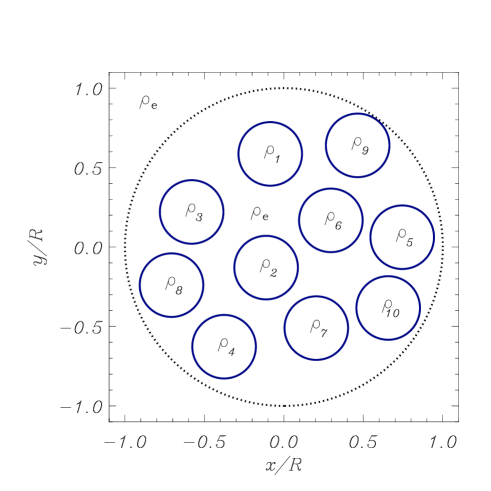
Figure 1: Sketch of the cross section of a multi-stranded loop model, which consists of a loop of radius $R$ (large dotted circle) filled with $N$ homogeneous strands of densities $\rho_{j}$ and radii $a$ (solid smaller circles). The external medium to the loop and the medium between strands consists of coronal material with density $\rho_{\mathrm{e}}$. It is important to note that the large dotted circle is not real and represents the external boundary of a hypothetical unresolved loop.

In order to compare the dynamics of a multi-stranded loop model with that of a monolithic tube, an equivalent flux tube is defined. The flux tube radius, $R$, corresponds to that of the cylinder that wraps the strand bundle (see Figure 1). The equivalent uniform density is

$$\rho_{\mathrm{eq}}=\sum_{j=1}^{N}\rho_{j}\left(\frac{a}{R}\right)^{2}+\rho_{\mathrm{e}}\left[1-N\left(\frac{a}{R}\right)^{2}\right]~{},$$ (1)

where the mass of the strand set and the coronal medium inside the hypothetical monolithic loop are considered. We have fixed the radius of the cylinder envelop to $R=0.03L$, a typical value for coronal loops (see Aschwanden et al., 2003). We have assumed the volume filled by the strands to be $40\%$ that of the monolithic loop. In addition, all the strands have the same radius. In this work, we have considered systems of $10$ and $40$ strands with radii $a=0.2R=0.006L$ and $a=0.1R=0.003L$, respectively.

3 Normal modes of ten identical strands

We first study a system of $N=10$ identical strands, i.e., with identical densities and radii. From the results of Luna et al. (2009), this is the situation for which the coupling between strands is stronger because all the tubes have identical individual kink frequencies, hereafter denoted by $\omega_{\mathrm{strand}}$. The density of each strand is fixed to $\rho_{j}=7.5\rho_{\mathrm{e}}$, which yields the equivalent density $\rho_{\mathrm{eq}}=3.6\rho_{\mathrm{e}}$ (see Equation (1)). The equivalent monolithic loop has an individual kink frequency $\omega_{\mathrm{mono}}=2.067v_{\mathrm{Ae}}/L$ computed with the fast wave dispersion relation in a cylinder (Edwin & Roberts, 1983), with $v_{\mathrm{Ae}}$ the Alfén speed in the coronal environment. Hereafter, all the frequencies are expressed in terms of this frequency. The individual kink frequency of each strand is then $\omega_{\mathrm{strand}}=0.737\omega_{\mathrm{mono}}$.

3.1 Frequency analysis of the collective normal modes

We have investigated the eigenfrequencies of the system and have found that they are distributed at both sides of the individual strand frequency and always below the frequency of the equivalent monolithic loop (see Figure 2(a)). The lowest and highest frequencies are $\omega=0.612\omega_{\mathrm{mono}}$ and $\omega=0.993\omega_{\mathrm{mono}}$, respectively. We see that the eigenfrequencies are in a broad band of width approximately $0.38\omega_{\mathrm{mono}}$. According to their spatial structure, we classify the normal modes in three groups. Modes with frequencies below the central frequency ($\omega\lesssim\omega_{\mathrm{strand}}$) are called low modes (left-hand side of the shaded area in Figure 2(a)). Mid modes are those with frequencies similar to the central frequency ($\omega\approx\omega_{\mathrm{strand}}$; shaded area in Figure 2(a)), and finally the solutions with $\omega\gtrsim\omega_{\mathrm{strand}}$ are referred to as high modes (right-hand side of the shaded area in Figure 2(a)). It is important to note that in a system of non-interacting strands the frequency of oscillation of each strand is $\omega_{\mathrm{strand}}$.

                                                                                                                                                                                                                                                                                            

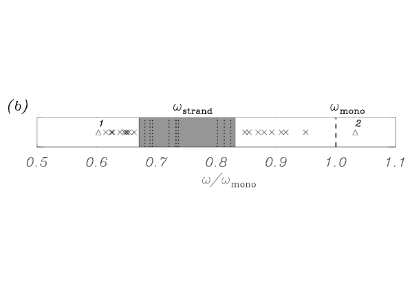
Figure 2: Frequency distribution of the collective normal modes associated to the three systems considered in this work: (a) $10$ identical strands, (b) $10$ nonidentical strands with different densities, and (c) $40$ identical strands. In all cases we clearly see that the frequencies are distributed at both sides of the individual strand frequencies, $\omega_{\mathrm{strand}}$, (dotted line) in a broad band of frequencies and that all modes have frequencies mainly below $\omega_{\mathrm{mono}}$ (dashed line). A shaded area is plotted between the lowest and largest mid mode frequencies. Then, mid modes lie within the shaded area, whereas low and high modes lie to its left and right, respectively. The triangles mark the frequencies of the modes whose spatial structure is displayed in the following plots and are labeled with integers.

3.2 Velocity and total pressure perturbation analysis

The spatial structure of the three groups of modes is clearly different. Low modes are kink-like modes in the sense that at least one strand moves transversely like in a kink mode of an individual loop. For these modes, the fluid between tubes follows the strand motion (see Figure 3), producing chains of loops in which one follows the next. In Figure 3, two examples of low modes are plotted. Figure 3(a) corresponds to the lowest frequency mode, in which only five strands oscillate, producing some kind of global torsional motion of the strands. In Figure 3(b) another example of low eigenfunction is plotted and it shows that almost all the strands are excited. As in the previous example, the fluid between strands moves with them. In both modes the maximum velocity takes place inside the strands. These characteristics are shared by all the low modes. The $S_{x}$ and $A_{y}$ modes of the system of two loops of Luna et al. (2008) and the $m_{1}$ to $m_{4}$ modes of a system of three aligned loops of Luna et al. (2009) can be classified in the low-mode group because the spatial structure of the magnetic pressure perturbation and velocity fields have the features previously described and their frequencies are below the corresponding individual kink frequency.

On the other hand, for the high modes (see Figure 4) the intermediate fluid between tubes is compressed or rarefied (which leads to a higher or lower total pressure perturbation) or moves in the opposite direction to the strands, producing a more forced motion than that of the low modes. High modes are kink-like too, but in contrast to the low modes the maximum velocities take place in the intermediate fluid between strands. This behavior is very clear in Figure 4(a), in which the strand motions force the coronal fluid to pass through the narrow channels between them or to compress the coronal medium. Similarly, in the highest frequency mode (Figure 4(b)), high velocity flows between the five excited strands takes place. The coronal medium within the excited strands is compressed and rarefied, giving rise to some kind of sausage global motion of the strands. All the modes that we have classified as high share these characteristics. The $S_{y}$ and $A_{x}$ modes of two identical tubes of Luna et al. (2008) and the $m_{5}$ to $m_{8}$ modes of a system of three aligned loops of Luna et al. (2008) belong to the high-mode group.

Finally, the mid modes have the most complex spatial structure. They are fluting-like modes and have strand motions similar to those of the fluting modes of an individual tube (see Figure 5). The magnetic pressure perturbation and velocity are concentrated mainly in the strand surface. There is an infinite number of mid modes with frequencies concentrated around $\omega\approx\omega_{\mathrm{strand}}$, and for this reason they are plotted as a shaded area in Figure 2.

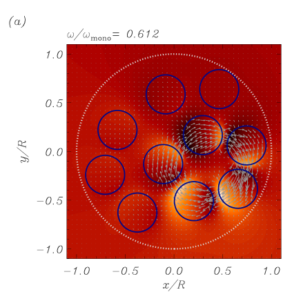
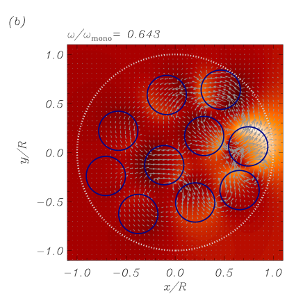
Figure 3: Total pressure perturbation (color field) and velocity field (arrows) of the fast collective normal modes of the two low modes labeled as $1$ and $2$ in Figure 2(a). (a) Lowest frequency mode labeled as $1$. (b) Low mode, labeled as $2$.

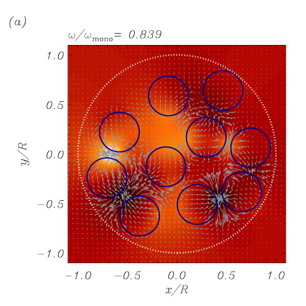
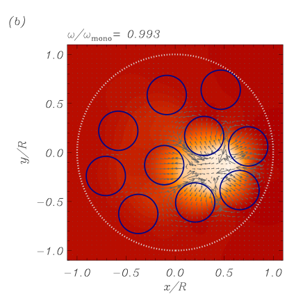
Figure 4: Same as Figure 3 for two high modes. (a) Mode labeled as $3$ in Figure 2(a). (b) Highest frequency mode, labeled as $4$.

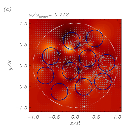
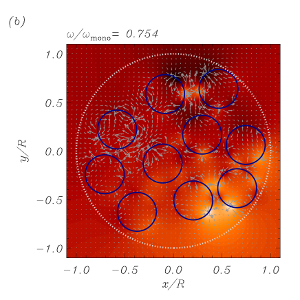
Figure 5: Same as Figure 3 for two mid modes. (a) Mode labeled as $5$ in Figure 2(a). (b) Mode labeled as $6$. In both cases we see the complex structure of the mid normal modes.

4 Normal modes of ten non-identical strands

In this Section we have considered the previous spatial distribution of strands but with different densities. The strand densities have been distributed randomly around and average density $7.5\rho_{\mathrm{e}}$ within a range of $3\rho_{\mathrm{e}}$. The equivalent monolithic density has been kept equal to $\rho_{\mathrm{eq}}=3.6\rho_{\mathrm{e}}$ and the volume filled by the strands to $40\%$ that of the monolithic loop volume, as in §3. The densities we use are $\rho_{j}/\rho_{\mathrm{e}}=\{7.89$, $7.61$, $7.60$, $8.97$, $5.98$, $8.73$, $7.52$, $8.62$, $6.18$, $5.80\}$ following the ordination of Figure 1. The considered range of strand densities implies that the difference between the maximum and minimum values of the individual kink frequencies is $0.13\omega_{\mathrm{mono}}$. This makes the coupling between the strands weaker (see Luna et al., 2009) than in the identical strand case discussed in §3. However, the strands still interact and so it is not possible to consider the multi-stranded system as a collection of individual tubes. The band of collective frequencies now goes from $\omega=0.602\omega_{\mathrm{mono}}$ to $\omega=1.036\omega_{\mathrm{mono}}$, i.e., it has a width of $0.43\omega_{\mathrm{mono}}$, as we see in Figure 2(b). This band is broader than in the identical strand case (for which it is $0.38\omega_{\mathrm{mono}}$), but this does not mean that the interaction between non-identical strands is stronger. The reason is the additional broadening associated to the spreading of the individual kink frequencies, which results in the enlargement of the mid frequency band (see Figure 2(b)). Roughly speaking, the broadening associated to the coupling is then the total broadening minus the spreading of the individual kink frequencies. In case of an uncoupled system of nonidentical strands the width of the band associated to the coupling is zero. The individual kink frequencies of our system are in a band of $0.13\omega_{\mathrm{mono}}$. This implies that the contribution of the strand interaction is roughly $0.30\omega_{\mathrm{mono}}$, indicating less interaction between the strands than for the identical strand system of §3. Similarly to §3, we can divide the collective normal modes in three groups (low, mid, and high). However, the spatial structure differs from those of the previous Section. The differences are clear, for example, in the lowest frequency mode. Comparing Figure 6(a) with Figure 3(a) we see that the global torsional oscillation of the five strands labeled $2$, $5$, $6$, $7$, and $10$ is avoided because their densities are very different, but the oscillation of the strands labeled as $1$, $2$, $3$, $4$, $6$, $7$, and $8$ with similar densities, is favored. The highest frequency mode plotted in Figure 6(b) is very similar to the corresponding mode in the identical tube case (Figure 4(b)), although the amplitude of the oscillations is concentrated in the rarest tubes, labeled $5$ and $10$. These results are general and so low modes have the largest oscillatory amplitudes in the denser tubes. On the contrary, for the high modes, the highest oscillatory amplitudes are associated to the rarest strands. Mid modes have a complex spatial structure but similar to that of the identical strand case and are not plotted for the sake of simplicity.

In Terradas et al. (2008) a system of $10$ non-homogeneous strands was considered. The authors studied the time-dependent evolution of the system after an initial excitation. They found a collective frequency $0.22/\tau_{\mathrm{A}}$, where $\tau_{\mathrm{A}}$ is defined as $\tau_{\mathrm{A}}=R/v_{\mathrm{Ae}}$. We have considered an equivalent system of homogeneous strands preserving the total mass and have found that modes lie in a frequency band going from $0.182/\tau_{\mathrm{A}}$ to $0.23/\tau_{\mathrm{A}}$ that agrees very well with the mentioned results.

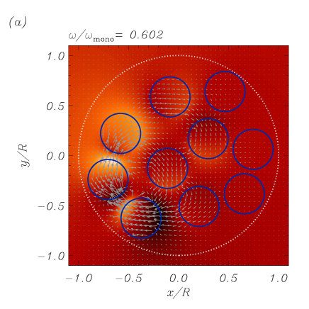
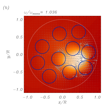
Figure 6: Same as Figure 3 for the collective normal modes of a system of $10$ non-identical strands. (a) Lowest frequency mode, labeled as $1$ in Figure 2(b). (b) Highest frequency mode, labeled as $2$.

5 Normal modes of forty identical strands

We have also investigated the normal modes of a much more complex system of $40$ identical strands. The strands fill $40\%$ of the equivalent loop volume, with a strand density $\rho_{j}=7.5\rho_{\mathrm{e}}$ and an equivalent density $\rho_{\mathrm{eq}}=3.6\rho_{\mathrm{e}}$. The frequencies of the normal modes lie in a band that goes from $\omega=0.614\omega_{\mathrm{mono}}$ to $\omega=0.987\omega_{\mathrm{mono}}$, so that its width is $0.37\omega_{\mathrm{mono}}$. This frequency band is similar to that of the $10$ identical strand case (see Figures 2(a) and 2(c)). However, the system of $40$ strands has more collective normal modes than the system of $10$ strands. The classification in low, mid, and high modes is still valid in this complex system of strands. In this Section we have only considered the kink-like modes (low and high modes) and the mid modes are not plotted for the sake of simplicity. In Figures 7(a) and 7(b), two examples of low collective normal modes are plotted. In the lowest frequency normal mode (Figure 7(a)), a cluster of close strands is excited and the others are at rest. In the second example (Figure 7(b)), a cluster of distant strands participate in the motion. In Figures 8(a) and 8(b), two examples of high modes are also plotted. Similarly to the low modes, in the high modes a cluster of several strands participates in the motion whereas the others are at rest.

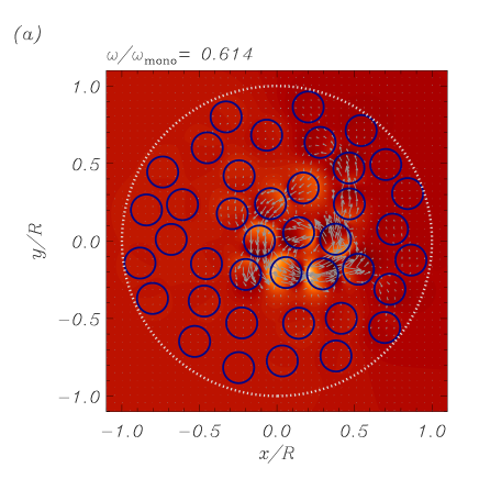
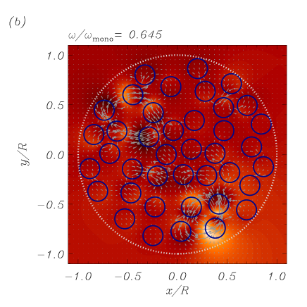
Figure 7: Same as Figure 3 for two low modes in a system of $40$ identical strands. (a) Lowest frequency mode, labeled as $1$ in Figure 2(c). (b) Normal mode labeled as $2$.

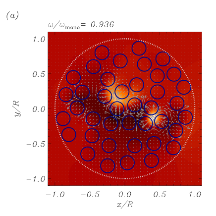
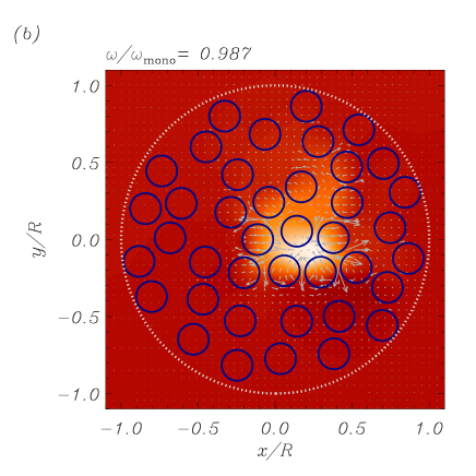
Figure 8: Same as Figure 3 for two high modes in a system of $40$ identical strands. (a) Collective normal mode, labeled as $3$ in Figure 2(c). (b) Highest frequency mode, labeled as $4$.

6 Time-dependent analysis: numerical simulations

In the previous sections we have considered the normal modes of a multi-stranded loop. Normal mode analysis provides information about the stationary state of the system or ideally, at an infinite time. However, loop oscillations are often produced by an impulsive event like a flare and it is more suitable to describe such events in terms of an initial value problem (see, e.g., Terradas, 2009). In addition, the time-dependent analysis gives information on how the different collective normal modes are excited and on how they are related with the temporal evolution after the initial disturbance.

We shall consider here the temporal evolution of the multi-stranded loop composed of $10$ identical strands of §3. The governing equations of the temporal evolution of the velocity field, $\mathbf{v}=\left(v_{x},v_{y},0\right)$, and magnetic field perturbation, $\mathbf{B}=\left(B_{x},B_{y},B_{z}\right)$, are the linearized ideal MHD equations, namely

$$\frac{\partial v_{x}}{\partial t} = \frac{v_{\mathrm{A}}^{2}}{B_{0}}\left(k_{z}~{}\widetilde{B}_{x}-\frac{\partial B_{z}}{\partial x}\right)~{},$$ (2)

$$\frac{\partial v_{y}}{\partial t} = \frac{v_{\mathrm{A}}^{2}}{B_{0}}\left(k_{z}~{}\widetilde{B}_{y}-\frac{\partial B_{z}}{\partial y}\right)~{},$$ (3)

$$\frac{\partial\widetilde{B}_{x}}{\partial t} = -~{}B_{0}~{}k_{z}~{}v_{x}~{},$$ (4)

$$\frac{\partial\widetilde{B}_{y}}{\partial t} = -~{}B_{0}~{}k_{z}~{}v_{y}~{},$$ (5)

$$\frac{\partial B_{z}}{\partial t} = -B_{0}\left(\frac{\partial v_{x}}{\partial x}+\frac{\partial v_{y}}{\partial y}\right)~{},$$ (6)

where $B_{x}=-i\widetilde{B}_{x}$ and $B_{y}=-i\widetilde{B}_{y}$ are purely imaginary variables. This fact indicates that the $x$- and $y$-components of the magnetic field have a phase lag of $\pm\pi/2$ with respect to the temporal evolution of the other variables.

The initial perturbation is a planar pulse in the velocity field of the form

$$\mathbf{v}_{0}=V_{0}~{}e^{-\left(y/w_{0}\right)^{2}}\mathbf{e}_{y},$$ (7)

(see arrows in Figure 9(a)) where $w_{0}$ is the width of the Gaussian profile, and $V_{0}$ is its amplitude. We have set the width of the initial perturbation equal to the loop radius, $w_{0}=R$, to perturb all the strands (see Figure 9(a)). In addition, we have chosen an amplitude of the perturbation, $V_{0}=0.02\,v_{\mathrm{Ae}}$, such that the maximum displacement of each strand is equal to the radius, $a=0.2R$. The initial value of the $x$-component of the velocity and the magnetic field perturbation are zero. Thus, the magnetic pressure is initially zero. We numerically solve the initial value problem with a code developed by J. Terradas based on the Osher-Chakrabarthy family of linear flux modification schemes (see Bona et al., 2009). The size of the simulated domain is $2R\times 2R$ and its boundaries are sufficiently far to neglect the effects of the reflections on the multi-stranded loop dynamics. The numerical mesh has $1000\times 1000$ grid-points and has enough resolution to resolve small scales and to avoid significant numerical diffusion.

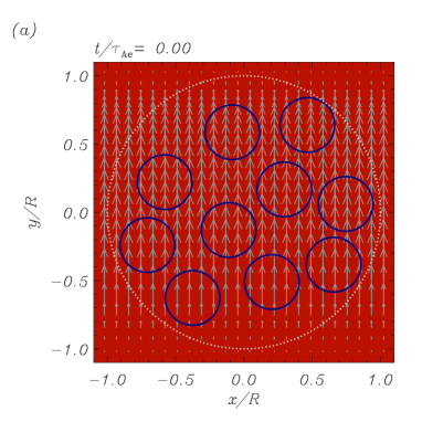
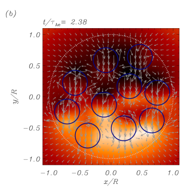
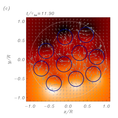
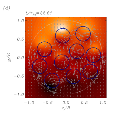
Figure 9: Time-evolution of the velocity field (arrows) and magnetic pressure perturbation (colored contours) for the system of $10$ identical strands of §3. The panels show different evolution times. In (a) the initial condition (Eq. 7) of the velocity field is plotted. In (b) the magnetic pressure and velocity fields are shown shortly after the initial disturbance. The initial pulse has left the domain shown in this panel and the system oscillates coherently. In (c) and (d) the structure of the fields indicate a complex motion of the strands. In (c) the direction of oscillation is completely different from that of the initial disturbance and in (d) the transverse displacement of the strands is mainly in the direction perpendicular to that of the initial pulse.

Figure 9 shows the temporal evolution of the magnetic pressure and velocity fields. The initial disturbance excites the $v_{y}$ component and the pulse front is on the $x$-axis (see Figure 9(a)). All the strands are excited at the same time and this produces the motion of the whole loop in the positive $y$-direction. In Figure 9(b), part of the perturbation energy has leaked from the system during the transient phase. The strands oscillate in the negative $y$-direction and in phase, in some kind of global-kink motion. The velocity field has a relatively simple structure, having a uniform value inside the strands. After some time, the spatial structure of the velocity and magnetic pressure perturbation fields are more complex (see Figure 9(c)). The polarization of the strand motion no longer parallel to the $y$-axis and each strand oscillates in its own direction. Similarly, in Figure 9(d) the velocity and magnetic pressure fields have also a complicated structure and the direction of oscillation of each strand has changed from that of Figure 9(c). Then, the initial value problem shows that the complexity of the magnetic pressure and velocity fields increases in time and that the simple spatial structure of Figure 9(b) is not recovered after the initial stage.

The temporal evolution of the velocity field indicates a complex motion of the strands. To show this more clearly, the trajectories of the strand centers are plotted with colored blue lines in Figure 10. Initially, all the strands oscillate in the $y$-direction, i.e., the direction of the initial disturbance. After a short time, the direction of the transverse oscillation of each strand changes and complicated trajectories arise. The motion of each strand produces a strong modulation of the whole loop transverse displacement. The trajectory of the center of mass (defined as $\mathbf{r}_{\mathrm{CM}}=\sum_{j=1}^{N}\mathbf{r}_{j}/N$) is plotted in Figure 10 as a colored red line. This trajectory represents the whole loop motion and it shows two effects. The first effect is that the initial linear polarization of the loop oscillation changes to a circular polarization in which the loop orbits around a central position. The second effect is an attenuation of the oscillation. The reason of this attenuation is that the non-organized motions contribute less to the whole loop motion than the initial organized motions. This behavior is even clearer in Figure 11 and the movie available in the electronic edition of the Journal. This figure shows the temporal evolution of the displacements of the strands with respect to their initial positions and also the displacement of the hypothetical monolithic loop.

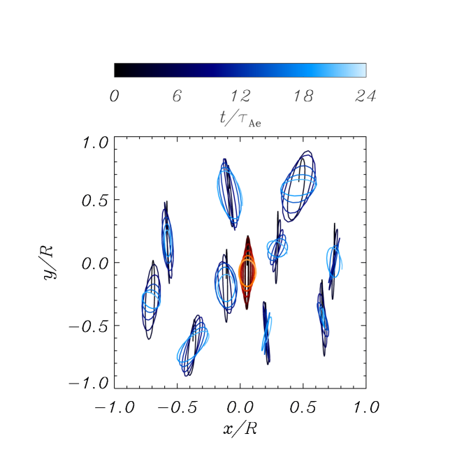
Figure 10: Plot of the trajectories of the strand centers (blue solid line) and the trajectory of the center of mass of the system (red solid lines). Time is represented by the color lightness of the curves start with dark color and end with light color (see color bar). The color bar associated to the motion of the center of mass is not plotted for the sake of simplicity. The strands and the center of mass start moving roughly parallel to the $y$-axis, but after some time the trajectories are ellipsis. To clarify the movements of the strands, the displacements are multiplied by two in this plot.

Figure 11: Time-evolution of the displacement of the strands (solid circles) and monolithic loop (large dotted circle). The initial position of the strands is also plotted as dashed circles. In (a) the maximum displacements of the strands exerted by the initial condition are plotted. All displacements are in the positive $y$-direction and in phase, indicating a coherent motion of the strand set. In (b) there is no privileged direction of oscillation, and complex motions of the strands are shown. The time of the two snapshots is displayed at the top of the figures. This figure is available as an mpeg animation in the electronic edition of The Astrophysical Journal.

In Figure 12, we have plotted the power spectrum of the magnetic pressure perturbation measured in a point located in the fluid between the strands. This figure shows that all the power is concentrated in the frequency band of the collective normal modes (see Figure 2(a)). This indicates that the initial disturbance excites a combination of collective normal modes (see §3). In general, the particular combination of normal modes depends on the shape, position, and incidence angle of the initial pulse (see Luna et al., 2008). With the particular initial disturbance of Equation (7), the power spectrum has the form of two peaks centered in the low and high frequency regions, while the power in the mid frequency region is small. Then, the initial disturbance largely excites the low and high frequency modes.

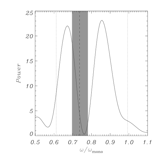
Figure 12: Power spectrum of the temporal evolution of the magnetic pressure perturbation measured at the position $(x/R,y/R)=(0.15,0.31)$. The left and right vertical dotted lines represent the frequencies of the lowest and highest frequency modes of Figure 2(a), respectively. The vertical dashed line is the kink frequency of the individual strands, $\omega_{\mathrm{strand}}$, while the shaded area, that corresponds to the shaded area in Figure 2(a), marks the region where mid modes reside. The power spectrum has two peaks in the low and high mode frequency ranges, which implies that the initial disturbance mainly excites the low and high frequency modes.

Ofman & Wang (2008) reported transverse oscillations of a multi-stranded loop. The system is made up of several close strands, and one may expect that the strands interact and oscillate with a combination of collective normal modes. Assuming that the system of strands is similar to that of §3, we can estimate the range of periods of collective normal modes. We use the mean values of the density and magnetic field obtained by the authors of $3\times 10^{9}~{}\mathrm{cm^{-3}}$ and $20~{}\mathrm{G}$, respectively. Also, imposing a reasonable external density of $4\times 10^{8}~{}\mathrm{cm^{-3}}$ (see Aschwanden et al., 2003), we keep the density contrast of our model ($\rho_{j}/\rho_{\mathrm{e}}=7.5$). With these values, the estimated collective periods range from $94~{}\mathrm{s}$ to $152~{}\mathrm{s}$, in good agreement with the $113~{}\mathrm{s}$ of the averaged oscillating periods of the strands measured by the authors. On the contrary, if the same system is assumed as a monolithic loop oscillating with a period of $113~{}\mathrm{s}$, the estimated magnetic field is $15~{}\mathrm{G}$. This very preliminary result shows that observations with poor spatial resolution tend to underestimate the magnetic field.

7 Discussion and conclusions

In this work we have studied analytically the normal modes of a multi-stranded coronal loop in the $\beta=0$ limit with the help of the $T$-matrix theory. We have also studied the temporal evolution of the system after an initial disturbance and its relation with the normal modes. The results of this work can be summarized as follows

1. We have considered a multi-stranded loop filled with $10$ identical strands located at random positions. We have found that the system supports a large quantity of normal modes whose frequencies are in a broad band of width approximately $0.38\omega_{\mathrm{mono}}$. All these frequencies are smaller than the monolithic kink frequency. The collective normal modes can be classified in three groups according to their frequencies and spatial structures. Low modes have a frequency $\omega\lesssim\omega_{\mathrm{strand}}$ and the spatial structure is kink-like and characterized by strands moving in complex chains. In these modes the intermediate fluid between strands follows their transverse displacement and this produces a non-forced motion of the system. In the low modes the strands move faster than the surrounding medium, i.e., the maximum velocities are within the strands. Mid modes have a frequency $\omega\approx\omega_{\mathrm{strand}}$ and the spatial structure is fluting-like, by which the strands are essentially distorted and their transverse displacements are small. Finally, high modes ($\omega\gtrsim\omega_{\mathrm{strand}}$) are kink-like modes characterized by a forced motion of the strands, that move in the opposite direction to the surrounding plasma or compress and rarefy their intermediate fluid, producing high velocities in the coronal medium. Then, the surrounding medium moves faster than the strands.

2. We have also investigated a system of $10$ non-identical strands. The spatial distribution of the strands is the same as in §3, but with different strand densities. Similarly to the identical strand case, we have found a large quantity of collective normal modes, but now their frequencies lie in a band of width $0.30\omega_{\mathrm{mono}}$. This band width is narrower than that of the identical strand case of §3, indicating a weaker interaction between the strands. The collective normal modes can be also classified in low, mid, and high modes. The largest oscillation amplitudes correspond to the denser strands in the low modes and to the rarest strands in the high modes.

3. The normal modes of a complex system of $40$ identical strands have also been computed. Their frequencies lie in a band of width $0.37\omega_{\mathrm{mono}}$ that coincides well with that of the system of $10$ identical strands. The classification of the normal modes in low, mid, and high is still valid in this complex system, although the number of normal modes is larger than in the two systems with $10$ strands. This indicates that the number of collective normal modes increases with the number of strands. In addition, these results indicate that the width of the frequency band does not depend strongly on the number of strands.

4. The temporal evolution of the system after an initial planar disturbance is also studied in the system of $10$ identical strands. Initially, the system oscillates in phase in the direction of the initial disturbance. After some time, this organized motion disappears and the complexity of the velocity and magnetic pressure perturbation fields increase. This implies a complex motion of the strands and, as a result, of the whole loop. In addition, we have found that the system oscillates with a combination of low and high collective normal modes.

In this investigation, we show that the transverse oscillation of a multi-stranded loop cannot be described by an equivalent monolithic loop. The reasons are that there is a huge quantity of normal modes with very different frequencies and very complex spatial structures. Their frequencies lie in a broad band and cannot be accounted for by an average frequency, because, after an initial disturbance most of the frequencies are excited. Furthermore, there is no collective normal mode that can be considered as a global kink mode, in which all the strands move in phase with the same direction and produce a transverse displacement of the whole loop. Instead, the collective normal modes that we have found displace the loop center but the detailed motion of the strands is very complex.

Additionally, the internal fine structure influences the whole loop dynamics. Complex motions of the strands are produced and also complex movements of the whole loop. These motions can be explained by the existence of a strong interaction between the strands and, consequently, the existence of a huge quantity of collective normal modes with different frequencies. The initial disturbance excites a particular combination of modes that causes a coherent motion of the strands similar to a global kink transverse oscillation. After some time, each collective normal mode oscillates with different phase due to the frequency differences between them. As a consequence the coherent motion of the strands is lost and complex motions appear. This behavior has already been shown by Luna et al. (2008) in a system of two identical flux tubes. The change of the initial linear polarization to a circular polarization of the whole loop transverse oscillation may be a signature of its internal fine structure. Circular transverse motion of a loop has been reported by Aschwanden (2009), who reconstructed the 3D motion by the curvature radius maximization method from TRACE images taken in the loop oscillation event of 1998 July 14. The author found that the horizontal and vertical oscillations have similar period and a phase delay of a quarter of a period. We suggest that the internal (thread) structure can contribute to the circular polarization and to the rapid damping of the transverse oscillations of coronal loops. We also show that the magnetic field strength tends to be underestimated in an observation of a multi-stranded loop oscillation in which the internal fine structure is not resolved. This result supports the findings of De Moortel & Pascoe (2009), who found that the estimated local magnetic field strength strongly depends on the theoretical model used to compare with the observations. Better models of coronal loop oscillations will improve the accuracy and reliability of the estimated magnetic fields obtained with the coronal seismology method. However, this is a preliminary study and more observations of circular transverse motions, a detailed study of the relation between the damping and the internal fine structure, and more high resolution measurements are needed. The recently launched Solar Dynamics Observatory (SDO) will provide new data with high spatial and temporal resolution. With these new observations better models of multi-stranded loops will be done.

In this work, we have made a number of simplifying assumptions, neglecting gas pressure, considering only linear perturbations, and ignoring gravity. In order to have more realistic models these effects need to be incorporated. Soler et al. (2009) have studied a system of two prominence threads with gas pressure and have found that transverse oscillations are coupled. These authors have also shown that slow modes are essentially individual modes. Then, we expect that the results shown here are still valid in a system with finite beta. Nevertheless, the addition of non-linear terms and gravity may introduce new effects that need to be addressed in a future research.

References

- Arregui et al. (2007) Arregui, I., Terradas, J., Oliver, R., & Ballester, J. L. 2007, A&A, 466, 1145
- Aschwanden et al. (1999) Aschwanden, M. J., Fletcher, L., Schrijver, C. J., & Alexander, D. 1999, ApJ, 520, 880
- Aschwanden et al. (2000) Aschwanden, M. J., Nightingale, R. W., & Alexander, D. 2000, ApJ, 541, 1059
- Aschwanden et al. (2003) Aschwanden, M. J., Nightingale, W., Andries, J., Goossens, M., & Van Doorsselaere, T. 2003, ApJ, 598, 1375
- Aschwanden (2009) Aschwanden, M. J. 2009, Space Science Reviews, 23
- Berton & Heyvaerts (1987) Berton, R., & Heyvaerts, J. 1987, Sol. Phys., 109, 201
- Bogdan & Cattaneo (1989) Bogdan, T. J., & Cattaneo, F. 1989, ApJ, 342, 545
- Bona et al. (2009) Bona, C., Bona-Casas, C., & Terradas, J. 2009, Journal of Computational Physics, 228, 2266
- De Moortel & Pascoe (2009) De Moortel, I., & Pascoe, D. J. 2009, ApJ, 699, L72
- Díaz et al. (2005) Díaz, A. J., Oliver, R., & Ballester, J. L. 2005, A&A, 440, 1167
- Edwin & Roberts (1983) Edwin, P. M., & Roberts, B. 1983, Sol. Phys., 88, 179
- Keppens et al. (1994) Keppens, R., Bogdan, T. M., & Goossens, M. 1994, ApJ, 436, 372
- Klimchuk (2006) Klimchuk, J. A. 2006, Sol. Phys., 234,41
- Lenz et al. (1999) Lenz, D. D., Deluca, E. E., Golub, L., Rosner, R., & Bookbinder, J. A. 1999, ApJ, 517, L155
- Litwin & Rosner (1993) Litwin, C., & Rosner, R. 1993, ApJ, 412, 375
- Luna et al. (2006) Luna M., Terradas J., Oliver R., & Ballester J. L. 2006, A&A, 457, 1071
- Luna et al. (2008) Luna M., Terradas J., Oliver R., & Ballester J. L. 2008, ApJ, 676, 717
- Luna et al. (2009) Luna M., Terradas J., Oliver R., & Ballester J. L. 2009, ApJ, 692, 1582
- Murawski (1993) Murawski, K. 1993, Acta Astronomica, 43, 2, 161
- Murawski & Roberts (1994) Murawski, K., & Roberts, B. 1994, Sol. Phys., 151, 305
- Nakariakov et al. (1999) Nakariakov, V. M., Ofman, L., DeLuca, E. E., Roberts, B., & Davila, J. M. 1999, Science, 285, 862
- Nakariakov & Ofman (2001) Nakariakov, V. M., & Ofman, L. 2001, A&A, 372, L53
- Ofman (2005) Ofman, L. 2005, Advances in Space Research, 36, 1572
- Ofman & Wang (2008) Ofman, L., & Wang, T. J. 2008, A&A, 482, L9
- Ofman (2009) Ofman, L. 2009, ApJ, 694, 502
- Reale & Peres (2000) Reale, F., & Peres, G. 2000, ApJ, 528, L45
- Roberts et al. (1984) Roberts, B., Edwin, P. M., & Benz, A. O. 1984, ApJ, 279, 857
- Schmelz et al. (2001) Schmelz, J. T., Scopes, R. T., Cirtain, J. W., Winter, H. D., & Allen, J. D. 2001, ApJ, 556, 896
- Soler et al. (2009) Soler, R., Oliver, R., & Ballester, J. L. 2009, ApJ, 693, 1601
- Terradas et al. (2008) Terradas, J., Arregui, R., Oliver, R., & Ballester, J. L. 2008, ApJ, 679, 1611
- Terradas (2009) Terradas, J. 2009, Space Science Reviews, 75
- Uchida (1970) Uchida, Y. 1970, PASJ, 22, 341
- Van Doorsselaere et al. (2008) Van Doorsselaere, T. 2008, A&A, 485, 849
- Wang et al. (2007) Wang, T., Innes, D. E., & Qiu, J. 2007, ApJ, 656, 598