The Coyote Universe III: Simulation Suite and Precision Emulator for the Nonlinear Matter Power Spectrum

Abstract

Many of the most exciting questions in astrophysics and cosmology, including the majority of observational probes of dark energy, rely on an understanding of the nonlinear regime of structure formation. In order to fully exploit the information available from this regime and to extract cosmological constraints, accurate theoretical predictions are needed. Currently such predictions can only be obtained from costly, precision numerical simulations. This paper is the third in a series aimed at constructing an accurate calibration of the nonlinear mass power spectrum on Mpc scales for a wide range of currently viable cosmological models, including dark energy. The first two papers addressed the numerical challenges, and the scheme by which an interpolator was built from a carefully chosen set of cosmological models. In this paper we introduce the “Coyote Universe” simulation suite which comprises nearly 1,000 $N$-body simulations at different force and mass resolutions, spanning 38 $w\,$CDM cosmologies. This large simulation suite enables us to construct a prediction scheme, or emulator, for the nonlinear matter power spectrum accurate at the percent level out to $k\simeq 1\,h\,{\rm Mpc}^{-1}$. We describe the construction of the emulator, explain the tests performed to ensure its accuracy, and discuss how the central ideas may be extended to a wider range of cosmological models and applications. A power spectrum emulator code is released publicly as part of this paper.

1. Introduction

During the last three decades, cosmology has made tremendous progress: from order of magnitude estimates to measurements of key cosmological parameters approaching percent level accuracy. The standard model of cosmology, based on the growth of structure by gravitational instability, has been impressively validated on large scales where the perturbations to the Friedman model are small. While the model is successful at predicting or reproducing a wide array of observations, it contains several mysterious elements with perhaps the most mysterious being the accelerated expansion of the Universe (Riess et al., 1998; Perlmutter et al., 1999). The accelerated expansion may be caused by a dark energy or hinting at a modification of general relativity on the largest scales.

To date most of the best known cosmological parameters have been constrained primarily from the study of anisotropies in the cosmic microwave background (CMB) radiation. However, large-scale structure probes play an important role in breaking parameter degeneracies and in constraining conditions in the late-time Universe. Such probes are becoming ever more precise, with future surveys aiming at measurements approaching percent level accuracy to better characterize the Universe in which we live. Techniques based on the observation and analysis of cosmic structure include the use of baryon acoustic oscillations, redshift space distortions, weak lensing measurements and the abundance of clusters of galaxies; they stand to play a pivotal role in improving our understanding of the dynamics of the Universe. (For a recent discussion regarding improvements on dark energy constraints from combining different probes, see, e.g. Albrecht et al. 2006, 2009). The large scale structure of the Universe contains information about both the geometry, as well as the dynamics of structure formation. In combination these two pieces of information can help distinguish between dark energy or a modification of general relativity as the prime cause of cosmic acceleration.

On small scales, the cosmological interpretation of structure formation probes is complicated due to the nonlinear physics involved. Commonly-used fitting functions for e.g., the power spectrum (Peacock & Dodds, 1996; Smith et al., 2003) have poorly characterized systematics and are no longer adequate for precision work. Absent a controlled theoretical framework, direct use of simulations (augmented with phenomenological parameters as appropriate) is essential if the physics is to be more correctly captured. The simulation codes need to be adequately tested to ensure they meet the new demands being placed upon them. The simulations which pass these goals are often very expensive and only a restricted number of runs can be performed. This in turn puts a premium on developing very efficient strategies to constrain parameters from limited observations and simulations. High-precision prediction schemes for different statistics are essential to succeed in this task.

Table 1The parameters for the 37+1 models which define the sample space; $k_{\rm nl}$ is measured in Mpc^-1. See text for further details.

#	$\omega_{m}$	$\omega_{b}$	$n_{s}$	$-w$	$\sigma_{8}$	$h$	$k_{\rm nl}^{z=0}$	$k_{\rm nl}^{z=1}$	#	$\omega_{m}$	$\omega_{b}$	$n_{s}$	$-w$	$\sigma_{8}$	$h$	$k_{\rm nl}^{z=0}$	$k_{\rm nl}^{z=1}$
M000	0.1296	0.0224	0.9700	1.000	0.8000	0.7200	0.12	0.19	M019	0.1279	0.0232	0.8629	1.184	0.6159	0.8120	0.15	0.24
M001	0.1539	0.0231	0.9468	0.816	0.8161	0.5977	0.11	0.18	M020	0.1290	0.0220	1.0242	0.797	0.7972	0.6442	0.11	0.18
M002	0.1460	0.0227	0.8952	0.758	0.8548	0.5970	0.10	0.17	M021	0.1335	0.0221	1.0371	1.165	0.6563	0.7601	0.16	0.25
M003	0.1324	0.0235	0.9984	0.874	0.8484	0.6763	0.11	0.17	M022	0.1505	0.0225	1.0500	1.107	0.7678	0.6736	0.13	0.22
M004	0.1381	0.0227	0.9339	1.087	0.7000	0.7204	0.14	0.22	M023	0.1211	0.0220	0.9016	1.261	0.6664	0.8694	0.15	0.23
M005	0.1358	0.0216	0.9726	1.242	0.8226	0.7669	0.12	0.20	M024	0.1302	0.0226	0.9532	1.300	0.6644	0.8380	0.16	0.24
M006	0.1516	0.0229	0.9145	1.223	0.6705	0.7040	0.14	0.24	M025	0.1494	0.0217	1.0113	0.719	0.7398	0.5724	0.12	0.20
M007	0.1268	0.0223	0.9210	0.700	0.7474	0.6189	0.11	0.18	M026	0.1347	0.0232	0.9081	0.952	0.7995	0.6931	0.11	0.18
M008	0.1448	0.0223	0.9855	1.203	0.8090	0.7218	0.12	0.20	M027	0.1369	0.0224	0.8500	0.836	0.7111	0.6387	0.12	0.19
M009	0.1392	0.0234	0.9790	0.739	0.6692	0.6127	0.13	0.21	M028	0.1527	0.0222	0.8694	0.932	0.8068	0.6189	0.11	0.18
M010	0.1403	0.0218	0.8565	0.990	0.7556	0.6695	0.12	0.19	M029	0.1256	0.0228	1.0435	0.913	0.7087	0.7067	0.13	0.21
M011	0.1437	0.0234	0.8823	1.126	0.7276	0.7177	0.13	0.21	M030	0.1234	0.0230	0.8758	0.777	0.6739	0.6626	0.12	0.19
M012	0.1223	0.0225	1.0048	0.971	0.6271	0.7396	0.15	0.24	M031	0.1550	0.0219	0.9919	1.068	0.7041	0.6394	0.13	0.23
M013	0.1482	0.0221	0.9597	0.855	0.6508	0.6107	0.14	0.23	M032	0.1200	0.0229	0.9661	1.048	0.7556	0.7901	0.13	0.19
M014	0.1471	0.0233	1.0306	1.010	0.7075	0.6688	0.14	0.23	M033	0.1399	0.0225	1.0407	1.147	0.8645	0.7286	0.12	0.19
M015	0.1415	0.0230	1.0177	1.281	0.7692	0.7737	0.14	0.22	M034	0.1497	0.0227	0.9239	1.000	0.8734	0.6510	0.11	0.18
M016	0.1245	0.0218	0.9403	1.145	0.7437	0.7929	0.13	0.20	M035	0.1485	0.0221	0.9604	0.853	0.8822	0.6100	0.10	0.17
M017	0.1426	0.0215	0.9274	0.893	0.6865	0.6305	0.13	0.21	M036	0.1216	0.0233	0.9387	0.706	0.8911	0.6421	0.09	0.15
M018	0.1313	0.0216	0.8887	1.029	0.6440	0.7136	0.14	0.23	M037	0.1495	0.0228	1.0233	1.294	0.9000	0.7313	0.12	0.19

This paper is the third in a series aimed at addressing this question in the context of the nonlinear matter power spectrum on Mpc scales. Current observations in weak lensing are quickly becoming theory limited due to the lack of precise theoretical estimates of this quantity for a wide range of cosmological models. This is a pressing problem. It is also relatively simple, allowing us to work through – in a concrete setting – the many steps which will be routinely required in the future. In some ways the problem is one of the simplest currently confronting theorists, but as we shall discuss below even it has demanded collaboration with other communities, the development of a significant infrastructure, new modes of working, and large amounts of manpower and computational capacity.

In Paper I of this series (Heitmann et al. 2009a) we demonstrated that it is possible to obtain nonlinear matter power spectra with percent level accuracy out to $k\simeq 1\,h\,{\rm Mpc}^{-1}$ and derived a set of requirements for such simulations. Paper II (Heitmann et al., 2009b) described the construction of an emulation scheme to predict the nonlinear matter power spectrum and the underlying cosmological models, building on the “Cosmic Calibration Framework” (Heitmann et al., 2006; Habib et al., 2007; Schneider et al., 2008). Here, in Paper III, we present results from the complete simulation suite based on the cosmologies presented in the second paper and publicly release a precision power spectrum emulator . The simulation suite is called the “Coyote Universe” after the cluster it has been carried out on. We will extend our work to include other measurements, such as the mass function or higher order statistics, in future publications.

The outline of this paper is as follows. In §2 we describe the simulations we have run in support of this program, and the codes with which they were run. §3 describes how we put together the different estimations of the power spectra from our multi-scale runs while §4 presents the details of the emulator and tests. We describe some lessons learned in §5 before concluding in §6.

2. The Simulation Suite

2.1. The Simulations

The Coyote Universe simulation suite encompasses nearly 1,000 simulations of varying force and mass resolution. The simulation volume is the same in all cases, a periodic cube of side length $1300\,$Mpc. We consider 37+1 cosmological models, listed in Table 1, which we select with two aspects in mind: our statistical framework and current constraints from a variety of cosmological measurements (see Paper II for further discussions and see below for a short summary).

The 37 models, labeled 1-37, are used to construct the emulator while model M000 is used as an independent check on the power spectrum accuracy in the parameter regime of most interest. (Other tests are described in §4 and in Paper II.)

For each cosmology we run 20 realizations, 16 lower resolution simulations covering the low-$k$ regime (which we refer to as the “L-series”), 4 medium resolution runs to provide good statistics in the quasi-linear to mildly nonlinear regime (the “H-series”), and one high resolution run to extend to $k\simeq 1\,h\,{\rm Mpc}^{-1}$ (the “G-series”). The high-resolution run uses the same realization as one of the medium resolution runs. The low- and medium-resolution runs are performed with a particle-mesh (PM) code. The code evolves $512^{3}$ particles in the low-resolution runs and $1024^{3}$ particles in the medium-resolution runs, in each case with a force mesh twice as large in each dimension as the particle load. Densities and forces are computed using Cloud-in-Cell (CIC) interpolation and a Fast Fourier Transform (FFT)-based Poisson solver. The potential is determined from the density using a $1/k^{2}$ Green’s function and the force is computed by $4^{\rm th}$ order differencing. Particles are advanced with second order (global) symplectic time-stepping with $\Delta\ln a=2\%$. In order to resolve the high-$k$ part of the power spectrum, we evolve one of the $1024^{3}$ particle initial distributions with the Tree-PM code GADGET-2 (Springel, 2005). We use a PM grid twice as large, in each dimension, as the number of particles, and a (Gaussian) smoothing of $1.5$ grid cells. The force matching is set to $6$ times the smoothing scale, the tree opening criterion to $0.5\%$ and the softening length to $50\,$kpc. The starting redshift for each simulation is $z=211$. Further details regarding the simulations and choices of simulation parameters can be found in Paper I.

All the simulations are carried out on Coyote, a large HPC Linux cluster consisting of 2580 AMD Opterons running at $2.6\,$GHz. The low-resolution PM runs are carried out on 64 processors, the medium-resolution PM runs and GADGET-2 runs on 256. For the billion particle runs we store particle and halo information at 11 different redshifts between $z=4$ and $z=0$. This leads to a final simulation database of size roughly $60\,$TB.

2.2. The Cosmological Models

The selection of the cosmological model suite depends on two considerations: the statistical framework we use to construct the emulator and current parameter constraints from the CMB as set by WMAP-5 (Komatsu et al., 2008). We do not insist on a formal methodology to make the model selection, but instead apply some practical and conservative arguments to justify our decisions. For an in-depth discussion we refer the reader to Paper II. In this paper we briefly summarize some of the considerations since these will define the region for which the emulator will be valid.

Our aim is to find a distribution of the parameter settings – the simulation design – which provides optimal coverage of the parameter space, using only a limited number of sampling points. Simulation designs well-suited for this task are Latin-Hypercube (LH)-based designs, a type of stratified sampling scheme. Latin hypercube sampling generalizes the Latin square for two variables, where only one sampling point can exist in each row and each column. A Latin hypercube sample – in arbitrary dimensions – consists of points stratified in each (axis-oriented) projection.

Very often LH designs are combined with other design strategies such as orthogonal array (OA)-based designs or are optimized in other ways, e.g., by symmetrizing them (more details below). By intelligently melding design strategies, different attributes of the individual sampling strategies can be combined to lead to improved designs, and shortcomings of specific designs can be eliminated. As a last step, optimization schemes are often applied to spread out the points evenly in a projected space. One such optimization scheme is based on minimizing the maximal distance between points in the parameter space, which will lead to more even coverage. Two design strategies well suited to cosmological applications in which the number of parameters is much less than the number of simulations that can be performed are optimal OA-LH design strategies and optimal symmetric LH design strategies. For this project, we have generated forty different designs following different strategies and chose the best design from these (where “best” refers to best coverage in parameter space with respect to specific distance criteria explained in Paper II).

In order to restrict the number of necessary simulation runs to an as small number as possible, it is helpful to keep the number of cosmological parameters and their prior ranges small. Current observations of the CMB and the large scale structure are consistent with a $\Lambda$CDM model with constant dark energy equation of state, $w$. We therefore concentrate on the following five cosmological parameters: $\omega_{m}\equiv\Omega_{m}h^{2}$, $\omega_{b}\equiv\Omega_{b}h^{2}$, $n_{s}$, $w$, and $\sigma_{8}$ where $\Omega_{m}$ contains the contributions from the dark matter and the baryons. We restrict ourselves to power-law models (no running of the spectral index) and to spatially flat models without massive neutrinos. For each cosmology, $h$ is determined by the angular scale of the acoustic peaks in the CMB (Paper II) which is known to very high accuracy (0.3%; Komatsu et al., 2008). From WMAP 5-year data, in combination with BAO, we have

$$\begin{array}[]{c}\omega_{m}=0.1347\pm 0.0040\quad(3\%),\\ \omega_{b}=0.0227\pm 0.0006\quad(3\%),\\ n_{s}=0.9610\pm 0.0140\quad(2\%).\end{array}$$ (1)

Current data restrict a constant equation of state for the dark energy to $w=-1$ with roughly 10% accuracy and recent determinations put the normalization in the range $0.7<\sigma_{8}<0.9$ with still rather large uncertainties.

Considering all these constraints and their uncertainties, we choose our sample space boundaries for the 37+1 models to lie within the range(s)

$$\begin{array}[]{c}0.120<\omega_{m}<0.155,\\ 0.0215<\omega_{b}<0.0235,\\ 0.85<n_{s}<1.05,\\ -1.30<w<-0.70,\\ 0.61<\sigma_{8}<0.9,\end{array}$$ (2)

over which the emulator is designed to produce reliable results. We verified in Paper II that 37 models spanning these parameter ranges are indeed enough to generate an emulator at the 1% accuracy. We emphasize that our emulator is valid for the complete parameter space defined by these priors and not restricted to some values in a band around the best-fit cosmology (for current observational data). Obviously, the emulator quality will be slightly worse on the edges of the hypercube but the emulator is always accurate within $\sim$1% anywhere within the priors.

2.3. Power Spectra

In Paper I we describe in detail how we obtain the matter power spectrum from a snapshot of the simulation. We briefly summarize the salient points here. We compute the dimensionless power spectrum,

$$\Delta^{2}(k)\equiv\frac{k^{3}P(k)}{2\pi^{2}},$$ (3)

which is the contribution to the variance of the density perturbations per $\ln k$. We obtain $\Delta^{2}$ by binning the particles onto a 2048³ grid using CIC assignment, applying an FFT, correcting for the charge-assignment window function, and averaging the result in fine bins in $|\mathbf{k}|$ spaced linearly with width $\Delta k\simeq 0.001\,{\rm Mpc}^{-1}$. As discussed in Paper I, we do not correct for particle discreteness as our particle loading is high enough to make such corrections unnecessary and there are some indications that a simple Poisson shot-noise form is not correct.

3. Power Spectrum Determination

When creating a nonlinear power spectrum emulator, we prefer that the underlying training data set be smooth. We describe here how we construct a smooth power spectrum from the 20 realizations of each cosmology and from cosmological perturbation theory.

In each simulation the modes in the initial density field are a single realization of a Gaussian random field and this introduces large run-to-run scatter. This scatter is reduced at higher $k$ by the relatively large number of modes which are averaged. However, at low $k$ the estimates of the power spectrum exhibit significant scatter which is expensive to reduce by brute force, i.e. running a very large number of realizations in large volumes. In addition, the approach to linear theory at low $k$ can be quite slow for many currently popular models around $\Lambda$CDM (if $1\%$ accuracy is the desired goal) so simply replacing the N-body results with the input linear model can be relatively inaccurate. This is however an area where perturbation theory can be of help, since the real-space mass power spectrum is computable in perturbation theory and there is a small but non-negligible range of scales where perturbation theory improves upon linear theory. For a recent overview of the performance of different perturbation theory approaches, see Carlson et al. (2009).

3.1. Perturbation theory

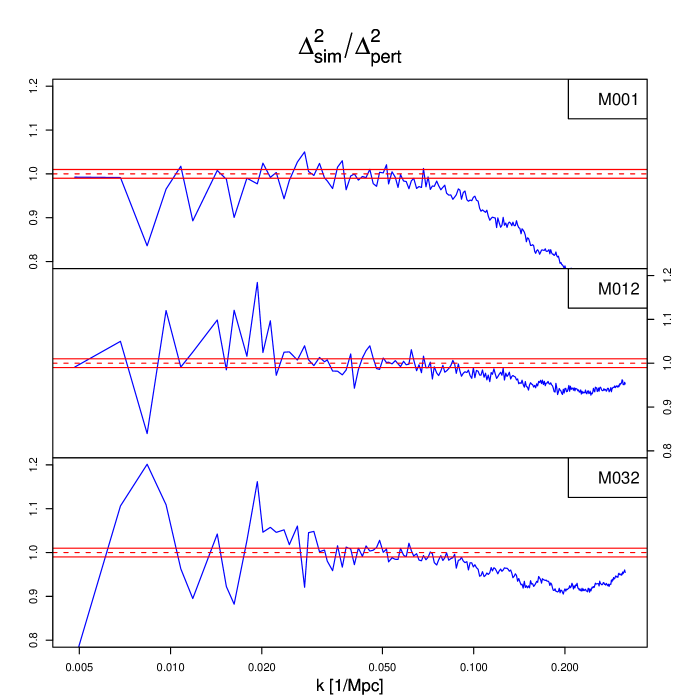
Figure 1.— Comparison of perturbation theory with the nonlinear matter power spectrum from simulations at $z=0$. Out of our 38 models we show three random examples, the results for the remaining models being very similar. For each model we determine a simulated power spectrum by matching the sixteen lower resolution L runs to the four medium resolution H runs at $k=0.25$ Mpc^-1. Therefore we average over 20 (1.3Gpc)³ simulations at low $k$-values and four simulations beyond $k=0.25$ Mpc^-1. We then take the ratio of the simulation results with respect to perturbation theory. The agreement is very good out to at least $k\simeq 0.03~{}$Mpc^-1. We therefore conclude that – up to these wavenumbers – perturbation theory results are robust for the cosmologies considered in this paper.

While there has been a resurgence of interest in perturbative methods in recent years, we stick to the simplest and oldest method: “standard perturbation theory” (Peebles, 1980; Juszkiewicz, 1981; Vishniac, 1983; Goroff et al., 1986; Makino et al., 1992; Jain & Bertschinger, 1994). We consider only the first correction to linear theory, which in standard perturbation theory can be written in terms of a simple integral over the linear theory power spectrum (we use the specific form given in Meiksin, White & Peacock 1999). When compared to our simulations, we find that standard perturbation theory is accurate at the percent level for $k<0.5\,k_{\rm nl}$ where $k_{\rm nl}$ can be defined as (Matsubara, 2008):

$$k_{\rm nl}^{-2}=\frac{1}{3}\int\frac{dk}{k}\ \frac{\Delta^{2}(k)}{k^{2}}.$$ (4)

The values for $k_{\rm nl}$ at $z=0$ and $z=1$ are listed for all models in Table 1. For example, for model M000, $k_{\rm nl}\simeq 0.1\,{\rm Mpc}^{-1}$ at $z=0$. Similar results have been reported in Matsubara (2008) and Carlson et al. (2009).

Almost any scheme that switches smoothly from standard perturbation theory to our N-body results around $0.5\,k_{\rm nl}$ produces results that agree at the percent level. At $z=0$, this would lead to a matching point between $k=0.045$ Mpc^-1 (M036) and $k=0.075$Mpc^-1 (M019). For simplicity we keep the matching point the same for all cosmologies. Since we have good statistics from our simulations at $k\simeq 0.03$ Mpc^-1 already, we choose this $k$ value as a very conservative matching point for all models. To verify this point, we compare our simulation results to perturbation theory for the different cosmologies. The simplest approach for this comparison is “brute force”: simply take the ratio of the simulation result to the perturbation theory prediction. The major obstacle here is the run-to-run scatter in the simulations. In order to overcome this problem, one can follow two routes: either incorporate fluctuations from the realization into the perturbation theory prediction, as done in Takahashi et al. (2008), or average over a large number of large volume simulations. We follow the second approach to avoid any ambiguities and systematic errors resulting from finite box size effects.

An example of our approach is shown in Figure 1 for a random subset of 3 models from the total of 37 used to build the emulator. Although at the lower end of the $k$ range, the large but finite sampling volume becomes clearly evident, the matching to perturbation theory at $k\simeq 0.03~{}$Mpc^-1 works extremely well. A similar result can also be found in Carlson et al. (2009).

3.2. The Estimation Procedure

Next, we show how we can combine perturbation theory and results from $N$-body simulations to generate smooth power spectra which will be the foundation for building our emulator. Two problems have to be solved for this: (1) We have to eliminate the scatter in the $N$-body results for the nonlinear power spectrum without erasing subtle features and match results from different resolution simulations. (2) We have to match very accurately between perturbation theory and simulation results. In the following, we discuss an approach based on process convolution to solve these problems.

3.2.1 Power Spectrum Estimation using Process Convolution

In this section, we discuss the procedure for estimating the smooth power spectrum for each cosmology based on the simulation results which possess inherent scatter. Figure 2 shows the power spectrum from the simulations for model M001 at $z=0$. The data have three notable features that are important for the modeling procedure. (1) The non-standard representation for the power spectrum

$${\cal P}(k)=\Delta^{2}(k)/k^{1.5}$$ (5)

is chosen to accentuate the baryon acoustic oscillations. We will account for this feature when we choose our function class for the smooth power spectra (discussed later). (2) The three series of simulations; G, H, and L with 1, 4, and 16 realizations respectively. Because the H and L series do not have enough force resolution to resolve the nonlinear regime at high $k$, we need to restrict the use of these runs to small and intermediate $k$ ranges. (3) The simulation variance at any given $k$ is known.

We treat each simulated (“noisy”) realization of the (large volume or averaged) spectrum as a draw from a multivariate Gaussian distribution whose mean is given by an unknown smooth spectrum. Thus, for a given cosmology $c$, a given series $s\in\{\mbox{G},\mbox{H},\mbox{L}\}$, and a given replicate $i=1,\cdots,N_{s}$ (where $N_{s}$ is the number of simulations for the series), we have a multivariate Gaussian density for the simulated spectrum $P^{c}_{s,i}$,

$$f(P^{c}_{s,i}) \propto \left|A_{s}\Omega A_{s}^{T}\right|^{1/2}$$

$$\times \exp\left\{-\frac{1}{2}\left(P^{c}_{s,i}-A_{s}\mathcal{P}^{c}\right)^{T}A_{s}\Omega A_{s}^{T}\left(P^{c}_{s,i}-A_{s}\mathcal{P}^{c}\right)\right\}.$$

Here, $\mathcal{P}^{c}$ is the smooth power spectrum; $A_{s}$ is a projection matrix of zeros and ones that is used to remove the high-$k$ values for which the H and L series are not used (thus, $A_{G}$ is an identity matrix); and $\Omega$ is a diagonal matrix of the known precisions (inverse variances).

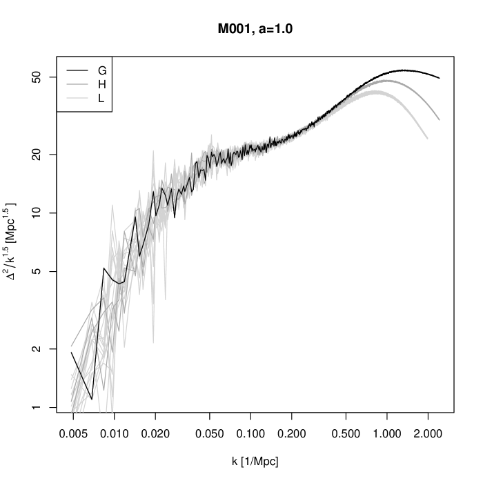
Figure 2.— Power spectra from the $N$-body simulations for cosmology M001 on the scales that are used for smoothing. The insufficient force resolution of the PM runs (H and L) is apparent at large $k$. To generate a smooth power spectrum over the whole $k$ range, we match perturbation theory and the L-runs at $k=0.03$ Mpc^-1, the L- and H-series at $k=0.25$ Mpc^-1, and use the G-series for $k\geq 0.32$ Mpc^-1. Note the non-standard representation of the power spectrum via $\Delta^{2}(k)/k^{1.5}$.

The model is completed by specifying a class of functions for the smooth power spectrum $\mathcal{P}^{c}$. We choose a flexible class of smooth functions called a process convolution (Higdon, 2002). These functions are best described constructively. A process convolution builds a smooth function as a moving average of a simple stochastic process like independent and identically-distributed (i.i.d.) Gaussian variates or Brownian motion. The moving average uses a smoothing kernel whose width is allowed to vary over the domain to account for nonstationarity (smoother in some regions, more wiggly in others). Figure 3 shows a simple example of a process convolution built on white noise smoothed with a Gaussian kernel.

We build the process convolution for $\mathcal{P}^{c}$ on Brownian motion $u^{c}$, with marginal variance $\tau^{2}_{u}$, realized on a sparse grid (relative to the power spectrum) of evenly spaced points, $x$ (the number of points is not important so long as it is large enough; we use 100),

$$f(u^{c})\propto\left|\frac{1}{\tau^{2}_{u}}W\right|^{1/2}\exp\left\{-\frac{u^{c\prime}Wu^{c}}{2\tau^{2}_{u}}\right\},$$ (7)

where $W$ is the Brownian precision matrix with diagonal equal to $[1~{}2~{}\cdots~{}2~{}1]$ and $-1$ on the first off-diagonals (this matrix cannot actually be inverted, but never has to be in the estimation). The Brownian motion is transformed into $\mathcal{P}^{c}$ by the smoothing matrix $K^{\sigma}$,

$$\mathcal{P}^{c}=K^{\sigma}u^{c}.$$ (8)

The smoothing matrix $K^{\sigma}$ is built using Gaussian kernels whose width varies smoothly across the domain. Thus, we have

$$K^{\sigma}_{i,j}=\frac{1}{\sqrt{2\pi\sigma^{2}_{i}}}\exp\left\{-\frac{\left(\log_{10}(k_{i})-x_{j}\right)^{2}}{2\sigma_{i}^{2}}\right\},$$ (9)

where $k_{i}$ is the $i$-th value of $k$ for which the power spectrum is computed.

In the description of $K^{\sigma}$, $\sigma$ is indexed to indicate that it changes over the domain. Intuitively, we want $\sigma$ to be small in the middle of the domain in order to capture the oscillations, but large elsewhere to smooth away the noise. In order to estimate this varying bandwidth parameter, we build a second process convolution model. This model is built on i.i.d. Gaussian variates $v$, with mean zero and variance $\tau^{2}_{v}$, observed on an even sparser grid of evenly spaced points, $t$ (length $M_{v}$; we use 10, but any large enough number will suffice),

$$f(v)\propto\left(\frac{1}{\sqrt{\tau_{v}^{2}}}\right)^{M_{v}}\exp\left\{-\frac{v^{\prime}v}{2\tau^{2}_{v}}\right\}.$$ (10)

The process $v$ is transformed into $\sigma$ by the smoothing matrix $K^{\delta}$,

$$\sigma=K^{\delta}v.$$ (11)

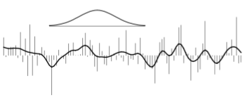
Figure 3.— The process convolution model treats a smooth function as arising from a weighted average of a simple stochastic process. In this figure, each point on the smooth function is a weighted average of the Gaussian impulses shown as the vertical bars. In these case, the weight function is a Gaussian kernel. Typically, the smooth function is observed (possibly with noise) and the challenge is to estimate the impulses and perhaps some aspect of the smoothing kernel.

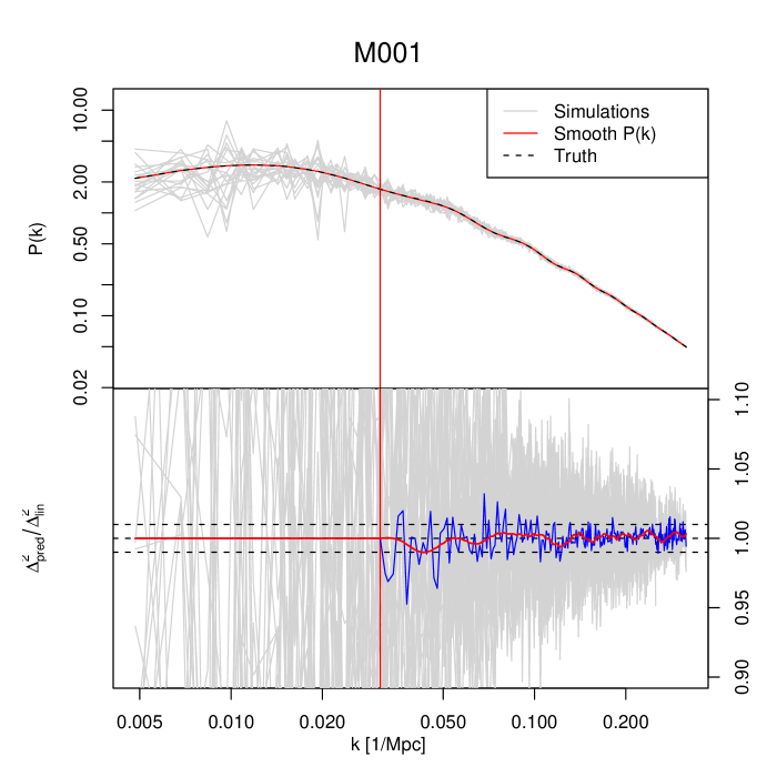
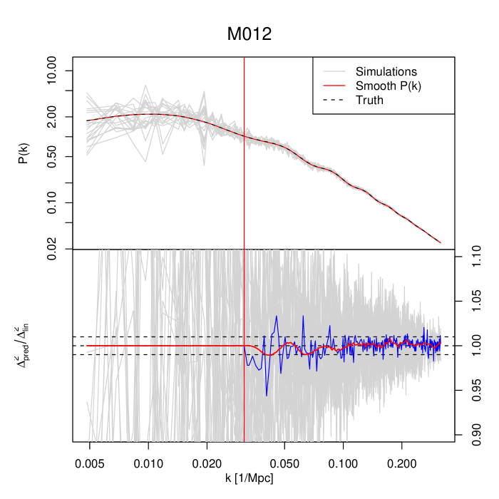
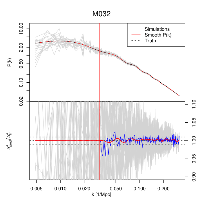
Figure 4.— Predictions for the linear power spectrum from 20 realizations of the initial power spectrum for the same three models shown in Figure 1. The upper panels for each model show in gray the realizations, in red the smooth power spectrum and in black (dashed) the linear theory power spectrum that underlies the simulations. The lower panels show the realizations (again in gray) divided by the linear theory answer and in red the smooth power spectrum divided by linear theory. The blue line shows the empirical mean of the realizations divided by linear theory. The vertical red lines in each panel indicate the matching point of linear theory and simulation result, the horizontal dashed lines in the lower panels show the 1% error. In all models the discrepancy is at the 1% level.

This matrix is also built using Gaussian smoothing kernels, but with a constant bandwidth, $\delta$. Thus, we have

$$K^{\delta}_{i,j}=\frac{1}{\sqrt{2\pi\delta^{2}}}\exp\left\{-\frac{\left(x_{i}-t_{j}\right)^{2}}{2\delta^{2}}\right\}.$$ (12)

Combining all of this, we get a distribution for the simulated power spectra for a given cosmology,

$$f(P^{c}_{s,i}) \propto \left|A_{s}\Omega A_{s}^{\prime}\right|^{1/2}$$

$$\times \exp\left\{-\frac{1}{2}\left(P^{c}_{s,i}-A_{s}K^{\sigma}u^{c}\right)^{\prime}A_{s}\Omega A_{s}^{\prime}\left(P^{c}_{s,i}-A_{s}K^{\sigma}u^{c}\right)\right\},$$

where $s\in\{\mbox{G},\mbox{H},\mbox{L}\}$ and $i=1,\cdots,N_{s}$. Note that $K^{\sigma}$ is a function of the parameters $v$ and $\delta$. We choose noninformative priors for $\tau^{2}_{u}$, $\tau^{2}_{v}$, and $\delta$ so as to impart little or no information about their values,

$$\pi(\tau^{2}_{u}) \propto \left(\frac{1}{\tau^{2}_{u}}\right)^{2}\exp\left(-\frac{.001}{\tau^{2}_{u}}\right),$$

$$\pi(\tau^{2}_{v}) \propto \left(\frac{1}{\tau^{2}_{v}}\right)^{2}\exp\left(-\frac{.001}{\tau^{2}_{v}}\right),$$ (14)

$$\pi(\delta) \propto I\{0\leq\delta\leq 10\},$$

which are inverse gamma, inverse gamma, and uniform, respectively.

Equations (7) (for all $c$), (10), and (3.2.1) are multiplied together with Eqn. (3.2.1) (for all $c$) to produce a posterior distribution for the unknown parameters and stochastic processes. Obtaining an estimate for the smooth power spectra requires an estimate for each of the parameters, the process $v$, and each of the processes $u^{c}$ for all $c$. Markov Chain Monte Carlo (MCMC) via the Metroplis-Hastings algorithm (Chib & Greenberg, 1995) produces a sample from the posterior distribution by drawing each parameter individually. The stochastic processes $u^{c}$ can be integrated out of the distribution, so the MCMC produces samples of the parameters as well as $v$. We use the posterior mean of the parameters to obtain a conditional mean for each of the $u^{c}$ which is then transformed into each of the $\mathcal{P}^{c}$.

The perturbation results are included by setting the low $k$ values for each of the simulated spectra in a given cosmology to the perturbation results and setting the precisions for these values to be very large. This is done prior to the estimation described here. The replication of these values in every simulation, combined with the large precisions, nearly forces the estimated result through these points. Further, the transition from the N-body results to the perturbation results will be relatively smooth as long as the two line up fairly well.

3.2.2 Tests with the Linear Power Spectrum

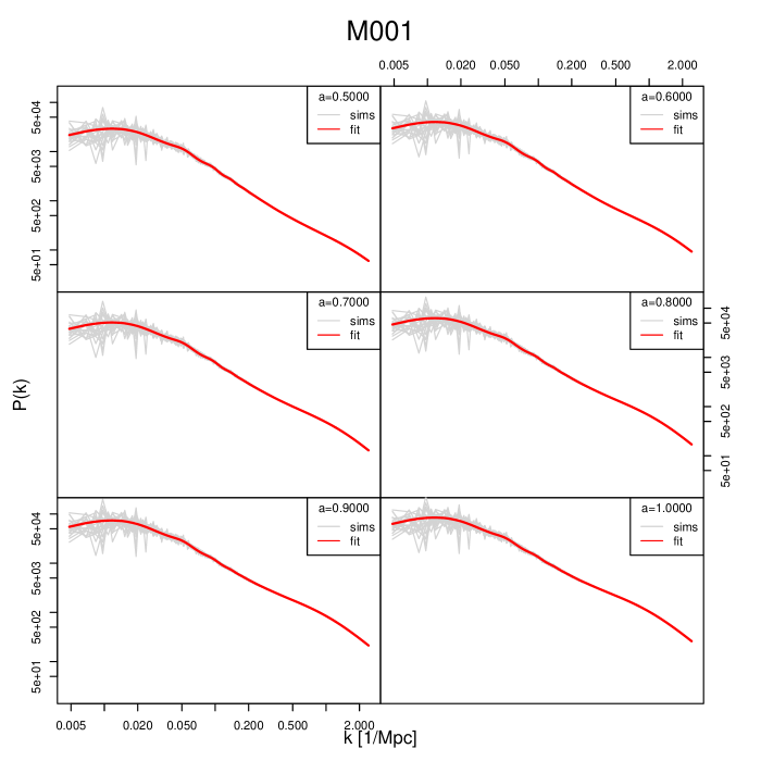
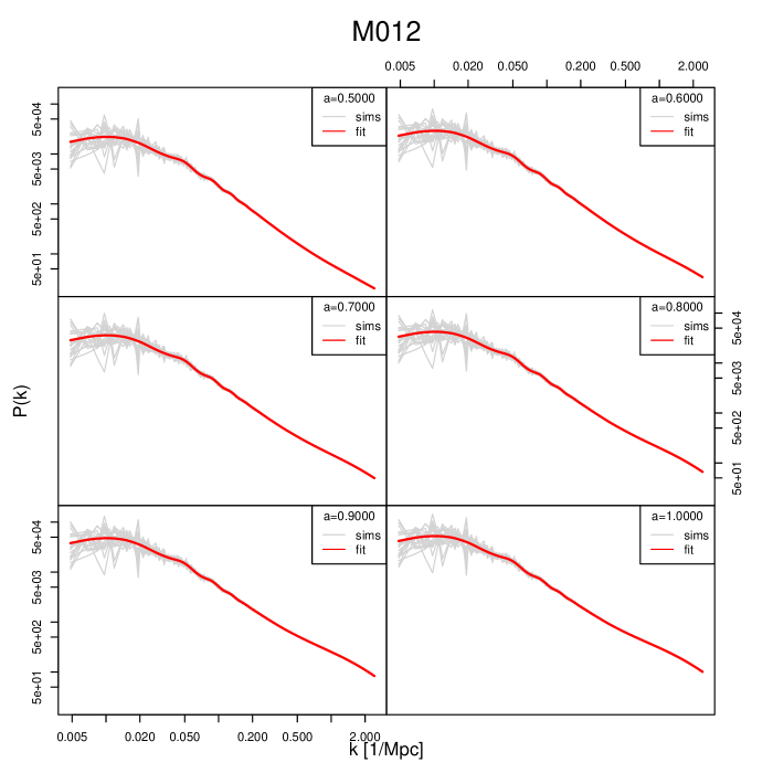
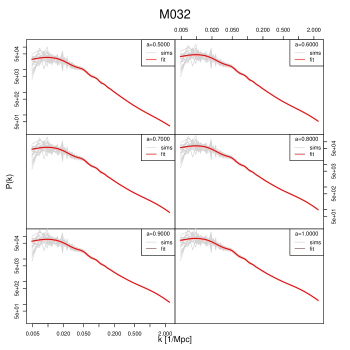
Figure 5.— Simulated power spectra and the smooth estimate for each of the three cosmologies at six values for the expansion factor $a$.

The next step is to test the matching procedure between theoretical and simulation results to ensure high accuracy at the perturbation theory matching point. Since we do not know the exact answer for the nonlinear power spectrum, we first carry out a test using linear theory. In this test we use the power spectra from the initial conditions and show how well we can smooth out the run-to-run scatter. Knowing the exact answer here will allow us to assess how well the matching procedure actually works.

For these spectra, the entire estimation procedure is applied to the initial condition spectra. The only difference is that fewer grid points were used for the latent processes $u$ and $v$ to account for the reduced range of the spectra (we use 70 and 7, respectively). The final results are shown in Figure 4 for the same set of three random models as in Figure 1. We verified that the results hold for all of the remaining models. The upper panels of each sub-panel show the theoretical linear power spectrum in black and the prediction from the simulations in red. The vertical line marks the matching point to linear theory at $k\simeq 0.03$Mpc^-1. The lower panels show the ratio of the predicted power spectra to the theoretical power spectra in red. Below the matching point, the agreement is – by construction – perfect. Beyond the matching point, the smoothed prediction in red is accurate at the 1% level. This test shows that we can obtain a smooth, high-accuracy prediction for the power spectrum by combining a suite of realizations with perturbation theory.

3.3. The Nonlinear Power Spectrum

The process convolution procedure is applied to the power spectrum realizations for each of the 37 cosmologies at six values of the scale factor $a=1/(1+z)\in\{0.5,0.6,0.7,0.8,0.9,1.0\}$, where $z$ is the redshift. The results are shown in Figure 5, again for a subset of three models. Although we have no known truth to use as a comparison in this case, the resulting estimates continue to fit the simulation realizations very well.

In place of comparing with known truth, we can examine some tests of our modeling assumptions. We assume that the simulation spectra on the modified scale are independently and normally distributed about a smooth mean with a variance that changes with $k$. Given this, we can compute standardized residuals in which the estimated smooth mean is subtracted from the simulations and the result is scaled by the known standard deviation. These standardized residuals should look like i.i.d. standard normal variables. Figure 6 shows quantile-quantile plots for the G simulations of three cosmologies at each of the six scale factors. Theoretical quantiles from a standard normal distribution are given on the $x$-axis and the sample quantiles of the standardized residuals are shown on the $y$-axis. The nearly straight line at $45^{\circ}$ indicates an extremely good distributional fit. Figure 7 shows the standardized residuals plotted against $k$ for the same simulations. This plot verifies the independence assumption. Further, there is an almost complete lack of evidence of any structure in these plots, suggesting that we would not greatly improve the fit by relaxing the smoothness assumption.

Figure 6.— Quantile-quantile plots of the standardized residuals for the G simulation at the six scale factors for three cosmologies. Standardized residuals are computed by subtracting the estimated mean from the simulation and multiplying each value by the square root of the known precision at its k value. Our assumptions suggest that the resulting sample should follow a standard normal distribution with no dependence on k. These plots show the sample quantiles of the standardized residuals (essentially the sorted values) plotted against the theoretical quantiles for a sample of this size from the standard normal distribution. The nearly straight lines indicate little deviation from our assumptions and suggest that the model fits well.

Figure 7.— The standardized residuals for the G simulation at the six scale factors for three cosmologies plotted against $k$. There are no obvious correlations or structure confirming our assumptions.

It is also interesting to examine the plot of the kernel width function as estimated by the MCMC process. Figure 8 shows the median draw for $\sigma$ as a function of $k$. As expected, the kernel width is small in the vicinity of the baryon wiggles. This means the values of the latent process $u$ in this region receive large weights, with the contributions for values further away dropping off very quickly. On both ends, the kernel width is large, which results in a smooth function in these regions.

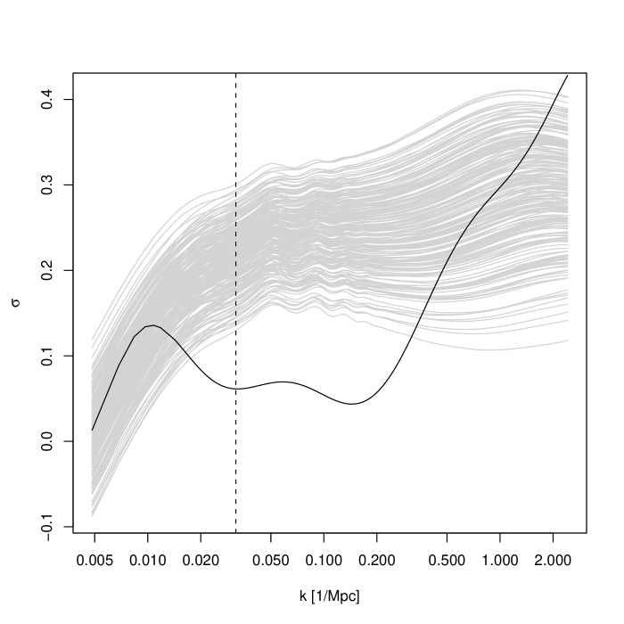
Figure 8.— Median MCMC draw for the bandwidth function $\sigma$ (black line). Small values on this plot correspond to places where the spectra are comparatively less smooth because of the baryon wiggles. In addition, all the power spectra are shown (37 models, 6 redshifts each) in light gray. The power spectra a scaled and shifted to fit the plot. $\sigma$ is low on the baryon acoustic oscillation scale to accommodate local wiggles, as expected. The vertical line shows the matching point between perturbation theory and the simulation outputs. On the left of this, each replicate is identical (compared to the realizations from the different simulation boxes) and smooth, therefore the behavior of $\sigma$ has not much information.

4. The Emulator

Having extracted the smooth power spectra from our simulation suite, we can now build an emulator to predict the nonlinear matter power spectrum within the priors specified in Eqns. (2). We will use only models 1 - 37 for the emulator construction; model M000 will serve as an independent check of the emulator accuracy, along with hold-out tests described below.

In order to construct the emulator, we model the 37 power spectra using an $n_{\mathcal{P}}$ dimensional basis representation:

$$\mathcal{P}(k;z;\theta)=\sum_{i=1}^{n_{\mathcal{P}}}\phi_{i}(k;z)w_{i}(\theta),~{}~{}~{}\theta\in[0,1]^{n_{\mathcal{\theta}}},$$ (15)

where the $\phi_{i}(k;z)$ are the basis functions, the $w_{i}(\theta)$ are the corresponding weights, and the $\theta$ represent the cosmological parameters. The dimensionality $n_{\mathcal{P}}$ refers to the number of orthogonal basis vectors $\{\phi_{i}(k,z),\dots,\phi_{n_{\mathcal{P}}}(k,z)\}$. The parameter $n_{\theta}$ is the dimensionality of our parameter space – with 5 cosmological parameters we have $n_{\theta}=5$. The power spectrum $\mathcal{P}(k;z;\theta)$ depends on the wavenumber $k$, the redshift $z$, and the five cosmological input parameters $\theta$ (note that we rescale the range of each parameter to $[0,1]$). Examination of the results indicates that $n_{\mathcal{P}}=5$ is a good choice for the number of basis vectors $\phi_{i}(k;z)$ (that $n_{\mathcal{P}}=n_{\theta}$ here is a coincidence). The task is now to (1) construct a suitable set of orthogonal basis vectors $\phi_{i}(k;z)$ and (2) model the weights $w_{i}(\theta)$). For the first task we use principal components, and for the second, Gaussian Process (GP) models. Our choice of GP modeling is based on their success in representing functions that change smoothly with parameter variation, e.g., the variation of the power spectrum as a function of cosmological parameters. Both steps are explained in great detail in Paper II; we refer the interested reader to that publication. Paper II also contains various error control tests of the GP-based interpolation method which we do not repeat here.

Since the details of how to build an emulator are already provided in Paper II we can immediately turn to our final product: the emulator itself. To facilitate use of the emulator, we are releasing the fully trained emulator with this paper. It provides nonlinear power spectra at a set of redshifts between $z=0$ and $z=1$ out to $k=1~{}h$Mpc^-1, for any cosmological model specified within the priors given in Eqns. (2).

4.1. Emulator Test

In order to verify the accuracy of the emulator, we perform two important checks (other tests on the methodology were carried out in Paper II). For the first, we compare the simulation results for model M000 with the emulator prediction. Figure 9 shows the results of this true out-of-sample prediction. The plot shows the ratio of the emulated power spectrum to the actual simulation for the M000 cosmology at six values of the scale factor $a$. This cosmology is completely interior in the design and, since M000 was not used to estimate the smoothing or the emulator, this test provides a good indication of the actual performance of the emulator within its parameter bounds. Overall the agreement between the simulations and the emulator is excellent and for most of the $k$-range well below the 1% error bound.

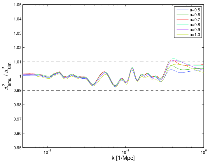
Figure 9.— Ratio of the emulator prediction to the smooth simulated power spectra for the M000 cosmology at six values of the scale factor $a$. The error exceeds 1% very slightly in only one part of the domain for the scale factors $a=0.7,0.8$, and 0.9.

The second check consists of a sequence of holdout tests. In a holdout test, the emulator is built from 36 cosmological models and the emulator prediction can be then compared to the result from the extra model. The drawback of this test is that if we have only a very small number of models, each of them is important for capturing some part of the parameter space and taking it out for building the emulator degrades the emulator precision. In order to keep this problem to a minimum, we only perform holdout tests for models which are interior simulations, meaning that none of the five parameters are near the extreme limits of the chosen prior range. There are six such models: M004, M008, M013, M016, M020, and M026. The ratio of the emulated prediction to the actual simulation for these models is shown in Figure 10. For each cosmology, there are six ratios for each value of the scale factor. The lines are quite well behaved with errors largely within the 1% bounds.

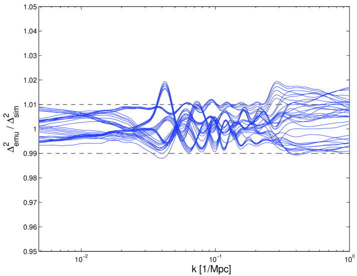
Figure 10.— M004, M008, M013, M016, M020, and M026. For each simulation, we show six residuals corresponding to the different values of the scale factor $a$. The errors are on the order of 1% for the bulk of the domain of interest. Considering that the tested emulators are built on an incomplete design, this result is remarkably good.

5. Lessons Learned and Future Challenges

The advent of precision cosmology and the prospect of very large surveys such as LSST and JDEM poses an enormous challenge to the theory community in the field of large scale structure predictions. Future progress not only requires very accurate predictions but also the ability to produce predictions for different cosmological models very fast. The aim of the Coyote Universe project was to take a first step in attacking this problem, focusing on the matter power spectrum at intermediate scales out to $k\simeq 1$ $h$Mpc^-1. While predicting the matter power spectrum on these scales at high accuracy may appear to be a moderately difficult task, it turned out to be a technical and computational challenge in several respects. It is generally hard to imagine problems and pitfalls in advance, which is why fully working through an example is so helpful. Since the community has to follow a similar path in the future to create predictive capabilities for different cosmological probes, we summarize here some of the lessons learned during this project.

The major differences between a project like this (including all three papers of the series) and previous numerical studies of large scale structure probes are:

(1) Computational and Storage Capacity: The Coyote Universe simulation suite encompasses roughly 60 TB of data. The computational cost is of the order of a million CPU-hours and including waiting times in submission queues, downtimes of the machine, and so on, carrying out these simulations took roughly six months. The simulation size of one billion particles in a Gpc³ volume was barely enough to resolve the scales of interest and for future work will certainly not be sufficient. Such simulations will need larger volumes and better mass resolution. For example, to resolve a 10¹²M_⊙ halo with 100 particles in a (3 Gpc)³ volume, we would need 300 billion particles. While supercomputers will get faster and larger in the future, generating many simulations at the edge of machine capabilities will always be a challenge. In addition, archiving the outputs of such simulations will become very expensive in terms of storage. From the Coyote Universe runs we stored 11 time snapshots plus the initial conditions (particle positions and velocities and halo information) leading to 250 GB of data per run. For the 300 billion particle run this would increase to 75 TB. Only very few places worldwide would be able to manage the resulting large databases.

(2) Simulation Infrastructure: Running a very large number of simulations makes it necessary to integrate the major parts of the analysis steps into the simulation code and to automate as much of the mechanics of running the code (submission, restarts) as possible. For the Coyote Universe project we developed several scripts to generate the input files of the codes, to structure the directories where different runs are performed in, and to submit the simulations to the computing queue system. For future efforts of this kind the adoption and development of dedicated workflow capabilities for these tasks must be considered. The number of tasks to be carried out will become too large to keep track of without such tools. In addition, since large projects will require extensive collaborations, software tools will make it easier to work in a team environment since each collaborator will have information about previous tasks and results. An example of such a tool for cosmological simulation analysis and visualization is given in Anderson et al. (2008).

We carried out the data analysis after the runs were finished. For very large simulations this is not very practical, and on-the-fly analysis tools are required to minimize read and write times and failures. This in turn requires that the code infrastructure be tailored to the problem under consideration.

(3) Serving the Data: Clearly, large simulation efforts cannot be carried out by a few individuals, and require possibly community wide coordination. The simulation data will be valuable for many different projects. It is therefore necessary to make the data from such simulation efforts publicly available and serve them in a way that new science can be extracted from different groups of simulations. Transferring large amounts of data is difficult because of limitations in communication bandwidth and also because of the large storage requirements. It would therefore be desirable to have computational resources dedicated to the database. In such a situation, researchers would be able to run their analysis codes on machines with direct access to the database and perform queries on the data easily. We are planning to make the Coyote Universe database available in the future and use it as a manageable testbed for such services.

(4) Communication with other Communities: The complexity of the analysis task makes it necessary to efficiently collaborate and communicate with other communities, for example statisticians, computer scientists, and applied mathematicians. Many tools that will be essential for precision cosmology in the future have already been invented – the task is to find them and use them in the best way possible.

6. Conclusions

This paper is the last of the Coyote Universe series of publications. Paper I was concerned with demonstrating that percent level accuracy in the (gravity only) nonlinear power spectrum could be attained out to $k\simeq 1$ Mpc^-1. Paper II showed that with only a relatively small number of simulations, interpolation across a high-dimensional space was possible at close to the same level of accuracy as that attained in the individual runs. Paper III takes this work to the final conclusion: Based on almost 1000 simulations spanning 38 $w$CDM cosmologies, we present a fast and very accurate prediction scheme – an emulator – for the nonlinear matter power spectrum. The emulator is accurate at the percent level, improving over commonly used fitting functions by almost an order of magnitude.

The emulator construction – as explained in Paper II – is based on GP modeling. In order to carry this out, a major challenge is to produce a smooth power spectrum from a finite set of simulations for each cosmology. In order to minimize run-to-run scatter on very large scales, we performed several medium resolution simulations and matched these at sufficiently low $k$ to perturbation theory. On quasi-linear scales we used medium resolution simulations and matched those to high resolution runs at small spatial scales. Matching the different resolution runs and perturbation theory accurately was carried out using process convolution. This technique allowed us to construct a smooth power spectrum for each cosmological model. The results were then used to construct the emulator via GP modeling as described in detail in Paper II.

We are releasing the power spectrum emulator as a C code, which allows the user to specify a cosmology within our priors and returns the power spectrum at six different redshifts between $z=0$ and $z=1$ out to $k\simeq 1$ Mpc^-1. These power spectra can now be used for further analysis of cosmological data. We are planning to extend the emulator in the near future to a larger $k$-range and will provide a smooth interpolation between results from different redshifts.

A major challenge will be to ensure that a certain level of accuracy is reached with the simulations when going to small scales. Besides being computationally very expensive (high force and mass resolution being required) the physics at smaller scales is far more complicated. The inclusion of gasdynamics and feedback effects (along with other physics) is far from being straightforward. The impossibility of carrying out a direct simulation effort is more or less certain; a good number of phenomenological/subgrid modeling parameters will be required. As simulation complexity and the number of modeling and cosmological parameters increases, it becomes even more important to develop efficient and controlled sampling schemes as described in Paper II, so that data can be used to determine both cosmological and modeling parameters (self-calibration).

With the series of three Coyote Universe papers we have demonstrated that it is possible to extract cosmological statistics such as the power spectrum at high accuracy and that one can build an accurate prediction scheme based on a limited set of simulations. This line of work will be important for interpreting results of future cosmological surveys. It will also have to be extended in several ways: (1) the cosmological model space has to be opened up; (2) we have to ensure high accuracy at scales smaller than those considered here; (3) we have to include more physics in order to capture those small scales correctly; (4) we have to include different cosmological probes, e.g., the cluster mass function and the shear power spectrum, to be able to build a complete framework for analyzing future survey data. We have shown here that such a program can in principle be established, though it will demand a large concerted effort between different communities.

References

- Albrecht et al. (2006) Albrecht, A. et al. 2006, arXiv:astro-ph/0609591.
- Albrecht et al. (2009) Albrecht, A. et al. 2009, arXiv:0901.0721.
- Anderson et al. (2008) Anderson, E., Silva, C., Ahrens, J., Heitmann, K., & Habib, S. 2008, Computing in Science and Engineering, 10, 30
- Carlson et al. (2009) Carlson, J.W., White, M., & Padmanabhan, N. 2009, Phys. Rev. D, 80, 043531
- Chib & Greenberg (1995) Chib, S. and Greenberg, E. 1995, The American Statistician, 49, 327
- Goroff et al. (1986) Goroff, M.H., Grinstein, B., Rey, S.-J., & Wise, M.B. 1986, ApJ, 311, 6
- Habib et al. (2007) Habib, S., Heitmann, K., Higdon, D., Nakhleh, C., & Williams, B. 2007, Phys. Rev. D, 76, 083503
- Heitmann et al. (2006) Heitmann, K., Higdon, D., Nakhleh, C., & Habib, S. 2006, ApJ 646, L1
- Heitmann et al. (2009a) Heitmann, K., White, M., Wagner, C., Habib, S., & Higdon, D., ApJ (submitted) [arXiv:0812.1052] (Paper I)
- Heitmann et al. (2009b) Heitmann, K., Higdon, D., White, M., Habib, S., Williams, B., & Wagner, C. 2009, ApJ, 705, 156 (Paper II)
- Higdon (2002) Higdon, D. 2002, Space and Space-Time Modeling Using Process Convolutions in Quantitative Methods for Current Environmental Issues (Springer)
- Jain & Bertschinger (1994) Jain, B. and Bertschinger, E. 1994, ApJ, 431, 495
- Juszkiewicz (1981) Juszkiewicz, R. 1981, MNRAS, 197, 931
- Komatsu et al. (2008) Komatsu, E. et al. 2009, ApJS, 180, 330
- Makino et al. (1992) Makino, N., Sasaki, M., & Suto, Y. 1992, PRD 46, 585
- Matsubara (2008) Matsubara, T. 2008, Phys. Rev. D, 77, 063530
- Meiksin, White & Peacock (1999) Meiksin, A., White, M., & Peacock, J.A. 1999, MNRAS, 304, 851
- Peacock & Dodds (1996) Peacock, J.A. and Dodds, S.J. 1996, MNRAS, 280, L19
- Peebles (1980) Peebles, P.J.E. 1980, The Large-Scale structure of the Universe, Princeton University Press (Princeton).
- Perlmutter et al. (1999) Perlmutter, S. et al. 1999, ApJ, 517, 565
- Riess et al. (1998) Riess, A.G, et al. 1998, AJ, 116, 1009
- Schneider et al. (2008) Schneider, M., Knox, L., Habib, S., Heitmann, K., Higdon, D., & Nakhleh, C. 2008, Phys. Rev. D, 78, 063529
- Smith et al. (2003) Smith, R.E., et al. [The Virgo Consortium Collaboration] 2003, MNRAS, 341, 1311
- Springel (2005) Springel, V. 2005, MNRAS, 364, 1105
- Takahashi et al. (2008) Takahashi, R. et al. 2008, MNRAS, 389, 1675
- Vishniac (1983) Vishniac, E. 1983, MNRAS, 203, 345