Magneto-optical Feshbach resonance: Controlling cold collision with quantum interference

Abstract

We propose a method of controlling two-atom interaction using both magnetic and laser fields. We analyse the role of quantum interference between magnetic and optical Feshbach resonances in controlling cold collision. In particular, we demonstrate that this method allows us to suppress inelastic and enhance elastic scattering cross sections. Quantum interference is shown to modify significantly the threshold behaviour and resonant interaction of ultracold atoms. Furthermore, we show that it is possible to manipulate not only the spherically symmetric s-wave interaction but also the anisotropic higher partial-wave interactions which are particularly important for high temperature superfluid or superconducting phases of matter.

1 Introduction

Two-particle interaction is a key to describing interacting many-particle systems at a microscopic level. Means of manipulating this interaction enable us to explore physics of such systems with controllable interaction. In solid state systems, the scope of externally controlling inter-particle interactions is limited due to crystalline structures. By contrast, ultracold atomic gases offer a unique opportunity since their interatomic s-wave interaction is widely tunable by a magnetic Feshbach resonance (MFR) [1]. New insight into the exotic phases of interacting electrons in solids can be gained from the experiments involving ultracold atoms with tunable interactions. Atom-atom interaction can also be manipulated by an optical Feshbach resonance (OFR) [2], albeit with limited efficiency. Over the last decade, MFR [3, 4] has been extensively used to study interacting Bose[5, 6, 7, 8] and Fermi gases[9, 10, 11] of atoms. Electric fields[12, 13] can also be used to alter interatomic interaction.

MFR relies on the interplay of Zeeman effects and hyperfine interactions while OFR is based on photoassociation (PA)[14, 15, 16] of two colliding ground state atoms into an excited molecular state. OFR has been demonstrated in recent experiments[17, 18, 19]. Recently, PA spectroscopy in the presence of an MFR has attracted a lot of attention both experimentally[20, 21, 22, 23] and theoretically[24, 25, 26, 27, 28]. Junker et al.[20] have observed asymmetric profile in PA spectrum under the influence of an MFR. This spectral asymmetry results from Fano-type quantum interference[29] in continuum-bound transitions[26]. The use of quantum interference to control Feshbach resonance had been suggested earlier by Harris[30]. Of late, quantum interference has been observed in two-photon PA[31, 32, 33] and coherent atom-molecule conversion[34]. It has also been shown that Fano’s theory[29] can account for PA spectrum[35, 36] even in the absence of any MFR.

Here we demonstrate theoretically a new method of altering two-atom interaction. Let us consider that a laser field is tuned near a PA transition of two atoms which are simultaneously influenced by a magnetic field-induced Feshbach resonance. There are two competing resonance processes occurring in this system. One is the MFR attempting to associate the two ground state atoms into a quasi-bound state embedded in the ground continuum. The other one is the PA resonance tending to bind the two atoms into an excited molecular state. PA transitions can occur in two competing pathways which originate from the perturbed and unperturbed continuum states. The Fano-type quantum interference between these two pathways can be used to control atom-atom interaction. This quantum control of two-body interaction due to applied magnetic and optical fields is what we call “magneto-optical Feshbach resonance” (MOFR). In strong-coupling regime of PA transitions, s-wave scattering state gets coupled to higher partial-wave states[37, 38] via two-photon continuum-bound dipole coupling. Since s-wave scattering amplitude is largely enhanced due to the applied magnetic field, amplitudes of the higher partial-waves coupled to s-wave will also be largely modified. By resorting to a model calculation, we present explicit analytical expressions for phase shifts, elastic and inelastic scattering rates which manifestly show the significant effects of quantum interference in controlling cold collision. Resonant interaction arises in many physical situations[39, 40, 41]. It is therefore important to devise coherent control of resonant interaction.

2 The model

As a simple model, we consider three-channel time-independent scattering of two homonuclear Alkali atoms in the presence of a magnetic and a PA laser field. Here channel implies asymptotic hyperfine or electronic states of the two atoms. There are two ground hyperfine channels of which one is energetically open (labeled as channel ‘1’) and the other one is closed (channel ‘2’) in the separated atom limit. Channel 3 belongs to an excited molecular state which asymptotically corresponds to two separated atoms with one ground and the other excited atom. We assume that the collision energy is close to the binding energy of a quasi-bound state supported by the ground closed channel. It is further assumed that the rotational energy spacing of the excited molecular levels is much larger than PA laser linewidth so that PA laser can effectively drives transitions to a single ro-vibrational level ($v,J$) of the excited molecule, where $v$ stands for vibrational and $J$ for rotational quantum numbers. The angular state of the two atoms in the molecular frame of reference can be written as $\mid J\Omega M\rangle=i^{J}\sqrt{\frac{2J+1}{8\pi^{2}}}{\cal D}^{(J)}_{M\Omega}(\hat{r})$ where $\Omega$ is the projection of the electronic angular momentum along the internuclear axis and $M$ is the z-component of J in the space-fixed coordinate (laboratory) frame. ${\cal D}^{(J)}_{M\Omega}(\hat{r})$ is the rotational matrix element with $\hat{r}$ representing the Euler angles for transformation from body-fixed to space-fixed frame. In our model, we assume that the PA laser is tuned near resonance of $J=1$ level of the excited molecule.

The energy-normalized dressed state of these three interacting states with energy eigenvalue $E$ can be written as

$$\Psi_{E} = \sum_{M}\frac{\phi_{vJM}(r)}{r}\mid e\rangle\mid J\Omega M\rangle+\frac{\chi(r)}{r}\mid g_{2}\rangle\mid 000\rangle$$ (1)

$$+ \int dE^{\prime}\beta_{E^{\prime}}\sum_{\ell m_{\ell}}\frac{\psi_{E^{\prime}\ell m_{\ell}}(r)}{r}\mid g_{1}\rangle\mid\ell 0m_{\ell}\rangle$$

where $\phi_{vJM}(r)$ is the radial part of the excited molecular state, $\chi(r)$ is the bound state in the closed channel and $\psi_{E^{\prime}\ell m_{\ell}}(r)$ represents energy-normalized scattering state of the partial wave $\ell$ with $m_{\ell}$ being the projection of $\ell$ along the space-fixed z-axis. $\mid g_{i}\rangle$ and $\mid e\rangle$ denote the internal electronic states of $i$-th ground and excited molecular channels, respectively. Here $E^{\prime}=\hbar^{2}k^{2}/(2\mu)$ is the collision energy, where $k$ and $\mu$ are the relative momentum and reduced mass of the two atoms, respectively. $\beta_{E^{\prime}}$ denotes density of states of the unperturbed continuum. Note that $\phi_{vJM}(r)$ and $\chi(r)$ are the perturbed bound states. In the limit $r\rightarrow\infty$, we have $r\Psi_{E}\rightarrow\int dE^{\prime}\beta_{E^{\prime}}\sum_{\ell m_{\ell}}\psi_{E^{\prime}\ell m_{\ell}}\mid g_{1}\rangle\mid\ell 0m_{\ell}\rangle$ and thus the scattering properties in MOFR are determined by the asymptotic behavior of $\psi_{E^{\prime}\ell m_{\ell}}$.

From time-independent Schrödinger equation, under Born-Oppenheimer approximation, we obtain the following coupled differential equations

$$\left[\hat{h}_{J}+V_{e}(r)-\hbar\delta_{1}-E-i\hbar\gamma_{J}/2\right]\phi_{vJM}$$ (2)

$$= -\sum_{\ell,m_{\ell}}\Lambda_{\ell m_{\ell},JM}^{(1)}\tilde{\psi}_{E\ell m_{\ell}}+\Lambda_{00,JM}^{(2)}\chi,$$

$$\left[\hat{h}_{0}+V_{2}(r)-E\right]\chi=-\sum_{M}\Lambda_{JM,00}^{(2)}\phi_{vJM}-V_{12}\tilde{\psi}_{E00}$$ (3)

$$\left[\hat{h}_{\ell}+V_{1}(r)-E\right]\tilde{\psi}_{E\ell m_{\ell}}= - \sum_{M}\Lambda_{\ell m_{\ell},JM}^{(1)}\phi_{vJM}$$ (4)

$$- \delta_{\ell 0}V_{12}\chi,$$

where $\tilde{\psi}_{E\ell m_{\ell}}=\int\beta_{E^{\prime}}dE^{\prime}\psi_{E^{\prime}\ell m_{\ell}}$, $\hat{h}_{J(\ell)}=-\frac{\hbar^{2}}{2\mu}\frac{d^{2}}{dr^{2}}+B_{J(\ell)}(r)$ with $B_{J(\ell)}(r)=\hbar^{2}/(2\mu r^{2})X_{J(\ell)}$ being the rotational term corresponding to $J(\ell)$. If the excited molecular potential $V_{e}$ belongs to Hund’s case (a) and (c), then $X_{J}=[J(J+1)-\Omega^{2}]$, otherwise $X_{J}=J(J+1)$ and $X_{\ell}=\ell(\ell+1)$. The laser couplings between different angular states are denoted by $\Lambda_{\ell m_{\ell},JM}^{(i)}=-\langle JM\Omega\mid\vec{D}_{i}.\vec{{\cal E}}_{PA}\mid\ell m_{\ell}0\rangle$, where $\vec{D}_{i}$ is the transition dipole moment between the excited and the ground $i$-th channel molecular electronic states. For homonuclear atoms, $V_{e}(r)$ goes as $-1/r^{3}$ and the ground potentials $V_{1}$ and $V_{2}$ behave as $-1/r^{6}$ in the limit $r\rightarrow\infty$. Here $\delta_{1}=\omega_{1}-\omega_{A}$ is the detuning between the laser frequency $\omega_{1}$ and the atomic resonance frequency $\omega_{A}$, $V_{1(2)}$ is the interatomic potential in channel 1(2), $\delta_{\ell 0}$ stands for Kronecker-$\delta$ and $V_{12}$ denotes spin-spin coupling between the two ground channels. We have here phenomenologically introduced the term $-i\hbar\gamma_{J}/2$ corresponding to the natural linewidth of the excited state $(v,J)$. The zero of the energy scale is taken to be the threshold of channel 1 and the atomic frequency $\omega_{A}$ corresponds to the threshold of the channel 3 (threshold of excited molecular potential). For simplicity, we assume that the excited state belongs to the $\Sigma$ symmetry. Then the dipole coupling between angular states provides $m_{\ell}=M$ and thus we can solve the above coupled equations for a given value of $M$. For notational convenience, we henceforth suppress the subscripts $M$ and $m_{\ell}$.

3 The solution

The coupled equations (2-4) can be conveniently solved by the method of Green’s function. Let $\phi_{vJ}^{0}$ be the excited bound state solution of the homogeneous part of (2) with binding energy $E_{vJ}$. Using the Green’s function $G_{vJ}(r,r^{\prime})=-\frac{\phi_{J}^{0}(r)\phi_{J}^{0}(r^{\prime})}{\Delta E_{vJ}+i\hbar\gamma_{J}/2}$ where $\Delta E_{vJ}=\hbar\delta_{1}+E-E_{vJ}$, we can write

$$\phi_{vJ}(r)=\frac{\int_{E^{\prime}}dE^{\prime}\beta_{E^{\prime}}\sum_{\ell}\Lambda_{E^{\prime}\ell,J}+\Lambda_{bb}}{\Delta E_{vJ}+i\hbar\gamma_{J}/2}\phi_{vJ}^{0}(r)$$ (5)

where $\Lambda_{E^{\prime}\ell,J}=\int dr^{\prime}\Lambda_{J,\ell}^{(1)}(r^{\prime})\phi_{J}^{0}(r^{\prime})\psi_{E^{\prime}\ell}(r^{\prime})$ is the free-bound dipole coupling between the unperturbed bound state $\phi_{vJ}^{0}$ and the perturbed scattering state $\psi_{E^{\prime}\ell}$ and $\Lambda_{bb}=\int dr^{\prime}\Lambda_{J,0}^{(2)}(r^{\prime})(r^{\prime})\phi_{vJ}^{0}(r^{\prime})\chi(r^{\prime})$ is the bound-bound dipole coupling between $\phi_{vJ}^{0}$ and the perturbed bound state $\chi$. Let $\chi^{0}(r)$ be the solution of the homogeneous part of (3) with binding energy $E_{\chi}$. Writing $\phi_{vJ}$ in the form $\phi_{vJ}=\int dE^{\prime}\beta_{E^{\prime}}A_{E^{\prime}}\phi_{vJ}^{0}$, we can express

$$\chi=\frac{1}{E-E_{\chi}}\int dE^{\prime}\beta_{E^{\prime}}\left(A_{E^{\prime}}|\Lambda_{bb}^{0}|^{2}+V_{E^{\prime}}\right)\chi^{0}(r)$$ (6)

where $\Lambda_{bb}^{0}$ is the Rabi frequency between the two bound states $\phi_{vJ}^{0}$ and $\chi^{0}$ and $V_{E^{\prime}}=\int dr^{\prime}\psi_{E^{\prime}0}(r^{\prime})V_{12}(r^{\prime})\chi^{0}(r^{\prime})$. Using this one can express $\Lambda_{bb}$ in terms of $\Lambda_{bb}^{0}$ and $V_{E^{\prime}}$. After having done some minor algebra, we obtain

$$A_{E^{\prime}}=\frac{(E-E_{\chi})\sum_{\ell}\Lambda_{E^{\prime}\ell,J}^{(1)}+V_{E^{\prime}}\Lambda_{bb}^{0}}{(E-E_{\chi})(\Delta E_{v1}+i\hbar\gamma_{J}/2)-|\Lambda_{bb}^{0}|^{2}}.$$ (7)

Note that the right hand side of (7) involves the laser coupling $\Lambda_{E^{\prime}\ell,J}^{(1)}$ with the perturbed continuum states. Here $A_{E^{\prime}}$ is related to the coefficient of $\phi_{vJ}^{0}$ in the energy-normalised dressed state (1) of three interacting states of which two are bound states and one is ground continuum state. Since $\phi_{vJ}^{0}$ is unit-normalised, $A_{E^{\prime}}$ has the dimension of inverse of square root of energy. Physically, PA excitation probability for collision energies ranging from $E^{\prime}$ to $E^{\prime}+dE^{\prime}$ is given by $|A_{E^{\prime}}|^{2}dE^{\prime}$. Now, substituting (7) into (5) and (6) and then using the resultant form of $\phi_{vJ}$ and $\chi$ into (4), it is easy to see that the equation of motion for particular $\ell$-wave function gets coupled to other $\ell$-wave functions.

The Green’s function for the homogeneous part of (4) can be written as ${\cal K}_{\ell}(r,r^{\prime})=-\pi\psi_{E\ell}^{0,reg}(r_{<})\psi_{E\ell}^{+}(r_{>})$ where $r_{<(>)}$ implies either $r$ or $r^{\prime}$ whichever is smaller (greater) than the other. Here $\psi_{E\ell}^{+}(r)=\psi_{E\ell}^{0,irr}+i\psi_{E\ell}^{0,reg}$ where $\psi_{E\ell}^{0,reg}$ and $\psi_{E\ell}^{0,irr}$ represent regular and irregular scattering wave functions, respectively, in the absence of optical and magnetic fields. Asymptotically, $\psi_{E\ell}^{0,reg}(r)\sim j_{\ell}\cos\eta_{\ell}-n_{\ell}\sin\eta_{\ell}$ and $\psi_{E\ell}^{0,irr}(r)\sim-(n_{\ell}\cos\eta_{\ell}+j_{\ell}\sin\eta_{\ell})$, where $j_{\ell}$ and $n_{\ell}$ are the spherical Bessel and Neumann functions for partial wave $\ell$ and $\eta_{\ell}$ is the phase shift in the absence of laser and magnetic field couplings. According to Wigner threshold laws, as $k\rightarrow 0$, $\eta_{\ell}\sim k^{2\ell+1}$ for $\ell\leq(n-3)/2$, otherwise $\eta_{\ell}\sim k^{n-2}$ with $n$ being the exponent of the inverse power-law potential at large separation. Using ${\cal K}_{\ell}(r,r^{\prime})$, the perturbed wave function $\psi_{E^{\prime}\ell\ell^{\prime}}$ can be formally expressed in terms of $V_{E^{\prime}}$, $A_{E^{\prime}}$ and $\Lambda_{bb}^{0}$ and the partial-wave free-bound dipole transition matrix elements $\Lambda_{E^{\prime}\ell,vJ}^{0}=\int dr\phi_{J}^{0}(r)\Lambda_{\ell,J}^{(1)}(r)\psi_{E^{\prime}}^{0}(r)$. Next, substituting this into (7) and the expression for $V_{E^{\prime}}$, we can express $A_{E^{\prime}}$ exclusively in terms of couplings between unperturbed states. Explicitly, we have

$$A_{E^{\prime}}=\frac{e^{i\eta_{0}}(q_{f}+\epsilon)/(\epsilon+i)\Lambda_{0}+\sum_{\ell\geq 1}e^{i\eta_{\ell}}\Lambda_{E^{\prime}\ell,vJ}^{0}}{{\cal D}-E_{q}^{shift}+i\hbar(\gamma_{J}+\Gamma_{q}+\sum_{\ell\geq 1}\Gamma_{J\ell})/2}$$ (8)

where $\Lambda_{0}=\Lambda_{E^{\prime}0,vJ}^{(1)}$, $\epsilon=[E-E_{\chi}-E_{\chi}^{shift}]/(\Gamma_{mf}/2)$ with $E_{\chi}^{shift}=\rm{Re}\int drV_{12}(r)\chi^{0}(r^{\prime})\int dr^{\prime}{\cal K}_{0}(r,r^{\prime})V_{12}^{*}(r^{\prime})\chi^{0}(r^{\prime})$ and $\Gamma_{mf}=2\pi\mid\int dr\psi_{E^{\prime},0}^{reg,0}(r)V_{12}(r)\chi^{0}(r)\mid^{2}=2\pi\mid V_{E^{\prime}}^{0}\mid^{2}$ being the MFR shift and line width, respectively. Here

$$q_{f}=\frac{V_{eff}+\Lambda_{bb}^{0}}{\pi\Lambda_{0}V_{E^{\prime}}^{0}}$$ (9)

is Fano’s $q$-parameter which is, in the present context, called ‘Feshbach asymmetry parameter’[26] with

$$V_{eff}=\rm{Re}\int dr\phi_{vJ}^{0}(r)\Lambda_{J\ell=0}^{(1)}(r)\int dr^{\prime}{\cal K}_{0}(r,r^{\prime})V_{12}(r^{\prime})\chi^{0}(r^{\prime})$$

being an effective potential acting between the two bound states as a result of their interactions with the s-wave part of the continuum states. In (8), ${\cal D}=\Delta E_{vJ}-\sum_{\ell}E_{J\ell}^{shift}$, $\Gamma_{J\ell}=2\pi|\Lambda_{E^{\prime}\ell,vJ}^{0}|^{2}$, $E_{J\ell}^{shift}=\rm{Re}\int dr\Lambda_{\ell,J}^{(1)}(r)\phi_{E^{\prime}\ell}^{0}(r^{\prime})\int dr^{\prime}{\cal K}_{\ell}(r,r^{\prime})\Lambda_{J,\ell}^{(1)}(r^{\prime})\phi_{E^{\prime}\ell}^{0}(r^{\prime})$,

$$\Gamma_{q}=\left[\frac{(q_{f}+\epsilon)^{2}}{\epsilon^{2}+1}\right]\Gamma_{J0}$$ (10)

and

$$E_{q}^{shift}=\left[\frac{\epsilon(q_{f}^{2}-1)-2q_{f}}{\epsilon^{2}+1}\right]\frac{\hbar\Gamma_{J0}}{2}.$$ (11)

Finally, we have

$$\psi_{E^{\prime}\ell} = e^{i\eta_{\ell}}\psi_{E^{\prime}\ell}^{0}+\frac{e^{i\eta_{0}}V_{E^{\prime}}^{0}+A_{E^{\prime}}(q_{f}-i)\pi\Lambda_{0}V_{E^{\prime}}^{0}}{(\epsilon+i)\Gamma_{f}/2}\delta_{\ell 0}$$ (12)

$$\times \int dr^{\prime}{\cal K}_{0}(r,r^{\prime})V_{12}(r^{\prime})\chi^{0}(r^{\prime})+A_{E^{\prime}}\int dr^{\prime}{\cal K_{\ell}}(r,r^{\prime})\Lambda_{\ell,J}^{(1)}(r^{\prime})\phi_{vJ}^{0}(r^{\prime})$$

where $\psi_{E\ell}^{0}=\psi_{E\ell}^{0,reg}$. The equations (8) and (12) constitute the solutions of our model.

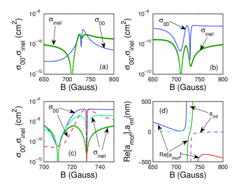
Figure 1: Subplots (a) and (b) show elastic and inelastic scattering cross sections $\sigma_{00}$ (solid line) and $\sigma_{inel}$ (solid-dotted line), respectively, in unit of cm² as a function of magnetic field $B$ in Gauss (G) for $\Gamma_{J0}/\gamma=0.1$ (a) and $\Gamma_{J0}/\gamma=10.0$ (b) at collision energy $E=10\mu$K and $q_{f}=-6.89$. Subplot (c) displays $\sigma_{00}$ Vs. $B$ (solid and dashed lines) and $\sigma_{inel}$ Vs. $B$ (dotted and solid-dotted lines) plots for $\Gamma_{J0}/\gamma=10.0$ (solid and solid-dotted lines) and $\Gamma_{J0}/\gamma=0.1$ (dashed and dotted lines) at $E=100$ nK and $q_{f}=-68.88$. Subplot (d) exhibits the variation of Re[$a_{mof}$] (solid line) and $a_{mf}$ (dashed lines) as a function of $B$ for $\Gamma_{J0}/\gamma=10.0$, $E=10\mu$K and $q_{f}=-6.89$. The other fixed parameters for all the subplots are $\Gamma_{mf}=16.67$ MHz and $\gamma=11.7$ MHz.

The elastic scattering amplitude is given by $f_{\ell\ell^{\prime}}=(1/2ik)(\delta_{\ell\ell^{\prime}}-S_{\ell\ell^{\prime}})=T_{\ell\ell^{\prime}}/k$ where the ${\mathbf{S}}$-matrix element $S_{\ell\ell^{\prime}}$ is related to the ${\mathbf{T}}-$matrix element $T_{\ell\ell^{\prime}}$ by $S_{\ell\ell^{\prime}}=\delta_{\ell\ell^{\prime}}-2iT_{\ell\ell^{\prime}}$. We can now derive $T_{\ell\ell^{\prime}}$ from the asymptotic behaviour the wave function of (12) which is given by $\psi_{E^{\prime}\ell}(r\rightarrow\infty)\sim\sin(kr-\ell^{\prime}\pi/2)\delta_{\ell\ell^{\prime}}-T_{\ell\ell^{\prime}}\exp(ikr-\ell\pi/2)$. The total elastic scattering cross section as $\sigma_{el}=\sum_{\ell^{\prime},m_{\ell^{\prime}}}\sum_{\ell,m_{\ell}}\sigma_{\ell\ell^{\prime}}$ where $\sigma_{\ell\ell^{\prime}}=4\pi g_{s}\mid T_{\ell\ell^{\prime}}\mid^{2}/k^{2}$, with $g_{s}=1$ for two distinguishable atoms and $g_{s}=2$ if the atoms are indistinguishable.

4 Results and discussions

4.1 Analytical results

We first consider the s-wave ($\ell=0$) scattered wave function. From the asymptotic form $\psi_{E^{\prime},0}\sim e^{i\eta_{0}}\psi_{E^{\prime},0}^{0,reg}-e^{i(kr+\eta_{0})}[e^{i\eta_{0}}+A_{E^{\prime}}(q_{f}+\epsilon)\pi\Lambda_{0}]/(\epsilon+i)$, we find $T_{00}=T_{0}^{0}+\exp(2i\eta_{0})T_{mf}+\exp[2i(\eta_{0}+\eta_{mf})]T_{q}=(1-S_{00})/2i$ where $T_{0}^{0}=-\exp(i\eta_{0})\sin\eta_{0}$, $T_{mf}=1/(\epsilon+i)=-\exp(i\eta_{mf})\sin\eta_{mf}$ where the MFR phase shift $\eta_{mf}$ is given by $\cot\eta_{mf}=-\epsilon$, $T_{q}=\Gamma_{q}/[{\cal D}-E_{q}^{shift}+i\hbar(\gamma_{J}+\Gamma_{J})]$. Here $\Gamma_{J}=\sum_{\ell}\Gamma_{J\ell}$. In the limit $k\rightarrow 0$, $\Gamma_{J\ell}\sim k^{2\ell+1}$ and hence $\Gamma_{J0}>\!>\Gamma_{J\ell\neq 0}$ for all $\ell\geq 1$. The ${\mathbf{S}}$-matrix element is $S_{00}=\exp(2i\eta_{tot})$, where $\eta_{tot}=\eta_{0}+\eta_{mf}+\eta_{q}$ with $\eta_{q}$ being a complex phase shift. Since in the limit $k\rightarrow 0$, $q_{f}\sim 1/k$, near MFR ($\epsilon\simeq 0$) the stimulated linewidth $\Gamma_{J}\simeq\Gamma_{q}\simeq q^{2}\Gamma_{J0}\sim 1/k$, $E_{q}^{shift}\simeq q_{f}\hbar\Gamma_{J0}$ and $\cot\eta_{q}=-[{\cal D}-E_{q}^{shift}+i\gamma_{J}]/\Gamma_{q}$. Thus in the limit $\gamma\rightarrow 0$ and $k\rightarrow 0$, $T_{00}$ fulfills unitarity.

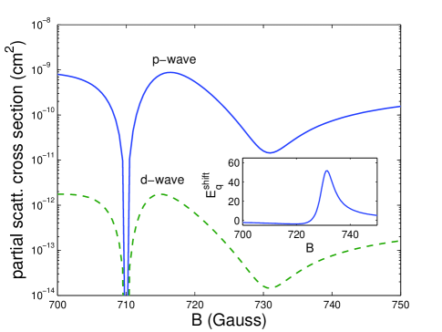
Figure 2: Partial-wave scattering cross section $\sigma_{\ell 0}$ is plotted as a function of $B$ for $\ell=1$ (solid line) and $\ell=2$ (dashed lines) for $\Gamma_{J0}/\gamma=10.0$, $\Gamma_{J1}=0.1\Gamma_{J0}$, $\Gamma_{J2}=10^{-4}\Gamma_{J0}$, $E=10\mu$K and $q_{f}=-6.89$. The inset shows $E_{q}^{shift}$ (in unit of $\hbar\Gamma_{mf}$) as a function of $B$ for the same parameters as in the main figure. The other parameters are same as in figure1

The s-wave elastic scattering cross section is $\sigma_{00}=g_{s}\pi\mid 1-S_{00}\mid^{2}/k^{2}$ and the inelastic cross section is $\sigma_{inel}=g_{s}\pi(1-\mid S_{00}\mid^{2})/k^{2}$. The corresponding rate coefficients are given by $K_{el}=\langle v_{rel}\sigma_{el}\rangle$ and $K_{inel}=\langle v_{rel}\sigma_{inel}\rangle$ where $\langle\cdots\rangle$ stands for thermal averaging over the relative velocity $v_{rel}=\hbar k/\mu$. Far from MFR ($\epsilon\rightarrow\pm\infty$) we have $T_{mf}\rightarrow 0$, $E_{q}^{shift}\rightarrow 0$ and $\Gamma_{q}\rightarrow\Gamma_{J0}$. In this limit $T_{q}$ reduces to the form $T_{of}=-\Gamma_{J0}/[{\cal D}+i\hbar(\gamma_{J}+\sum_{\ell}\Gamma_{J\ell}]$ which is the ${\mathbf{T}}$-matrix element of standard OFR for which both elastic and inelastic scattering rates increase as laser intensity increases [42].

We can define an energy-dependent complex MOFR scattering length by $a_{mof}=-\tan\eta_{tot}/k$. In the limit $k\rightarrow 0$ we have

$$a_{mof}\simeq\frac{a_{mf}+q_{f}^{2}\hbar\Gamma_{J0}/[k({\cal D}-E_{q}^{shift}+i\hbar\gamma_{J})]}{1+ka_{mf}q_{f}^{2}\hbar\Gamma_{J0}/({\cal D}-E_{q}^{shift}+i\hbar\gamma_{J})}$$ (13)

where $a_{mf}=-\lim_{k\rightarrow 0}\tan\eta_{mf}/k$ is the MFR scattering length. Since $(kq_{f}^{2}\Gamma_{J0})$ tends to be independent of $k$ at ultralow energy, it is possible to have the condition Re$[ka_{mf}q_{f}^{2}\hbar\Gamma_{J0}/({\cal D}-E_{q}^{shift}+i\hbar\gamma_{J})]>\!>1$ satisfied near MFR ($a_{mf}\rightarrow\pm\infty$) and PA resonance (${\cal D}\simeq 0$) in the strong-coupling regime ($\Gamma_{J0}>\!>\gamma_{J})$. Note that ${\cal D}=\Delta E_{vJ}-\sum_{\ell}E_{J\ell}^{shift}=0$ is the PA resonance condition in the absence of MFR. Furthermore, it is to be noted that $E_{q}^{shift}$ as given by (11) is independent of $k$ in the limit $k\rightarrow 0$ and $\epsilon\rightarrow 0$ and can greatly exceed the spontaneous linewidth $\gamma_{J}$ in the strong-coupling regime[27]. Under such conditions, we can write

$$a_{mof}\simeq\left(\frac{{\cal D}-E_{q}^{shift}}{kq_{f}^{2}\hbar\Gamma_{J0}}+\frac{1}{k^{2}a_{mf}}\right)+i\left(\frac{\gamma_{J}}{kq_{f}^{2}\Gamma_{J0}}\right).$$ (14)

Let us recall that $a_{mf}=-1/(k\epsilon)=-\hbar\Gamma_{mf}/[2k(E^{\prime}-\tilde{E}_{\chi})]$, where $\tilde{E}_{\chi}=E_{\chi}+E_{\chi}^{shift}$ and $E^{\prime}=\hbar^{2}k^{2}/(2\mu)$. Therefore, in the case of finite $\tilde{E}_{\chi}>E^{\prime}$, the real part of $a_{mof}$ (Re[$a_{mof}$]) becomes inversely proportional to energy and hence $\sigma_{el}\sim 1/k^{4}$ as $k\rightarrow 0$. In the case of $\tilde{E}_{\chi}=0$, Re[$a_{mof}$] goes to a constant in the limit $k\rightarrow 0$. In both the cases, the imaginary part of $a_{mof}$ (Im$[a_{mof}]$) becomes independent of $k$ but inversely proportional to laser intensity suggesting that $K_{inel}$ can be made very small by increasing the laser intensity. On the other hand, for ${\cal D}=0$, the (14) indicates that Re$[a_{mof}]$ becomes independent of laser intensity. Thus we can infer that the inelastic scattering rate can be suppressed while elastic rate can be enhanced by using quantum interference in the strong-coupling regime at ultralow temperatures. Very recently, Bauer et al. [23, 43] have experimentally demonstrated the effect of suppression of inelastic rate in PA due to the influence of a magnetic Feshbach resonance.

The amplitudes of higher partial-wave scattered wavefunctions can also be enhanced by MOFR. The higher partial waves that can be manipulated are given by the condition $\vec{J}=\vec{L}+\vec{S}+\vec{\ell}$. In the case of singlet to singlet PA transition for $J=1$, the maximum partial-wave that can be significantly affected is $\ell=2$ (d-wave), while in the case of triplet to triplet transition it is $\ell=3$. For $\ell\neq 0$, we have $T_{\ell 0}=\pi A_{E^{\prime}}\exp(i\eta_{\ell})\Lambda_{E\ell,vJ}^{0}$. Using (8), in the leading order in dipole coupling at ultralow energy we have

$$T_{\ell 0}\simeq\frac{e^{i(\eta_{0}+\eta_{\ell})}(q_{f}+\epsilon)/(\epsilon+i)\pi\Lambda_{0}\Lambda_{E\ell,vJ}^{0}}{{\cal D}-E_{q}^{shift}+i\hbar(\gamma_{J}+\Gamma_{q})/2}$$ (15)

In the limit $\epsilon\rightarrow\infty$, $T_{\ell,0}$ reduces to that of OFR[37] for $\ell\geq 1$

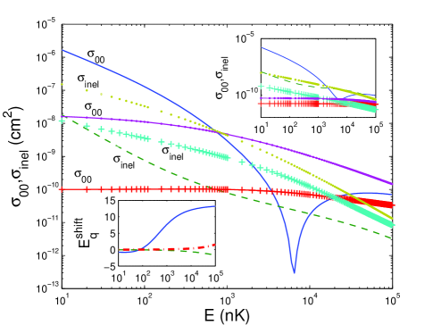
Figure 3: $\sigma_{00}$ and $\sigma_{inel}$ are plotted as a function of collision energy $E$ (in nK) for $B=730$ G (solid and dashed curves), $B=700$ G (plus-solid and plus curves) and $B=800$ G (solid-dotted and dotted curves) with $\Gamma_{J0}/\Gamma_{mf}=1.4$. The upper inset shows the same but for $\Gamma_{J0}/\Gamma_{mf}=0.07$. In the lower inset, $E_{q}^{shift}$ (in unit of $\hbar\gamma$) is plotted against $E$ for $B=730$ G (solid line), $B=700$ G (dotted line) and $B=800$ G (dashed lines) with $\Gamma_{J0}/\Gamma_{mf}=1.4$. The other parameters remain same as in figure1

4.2 Numerical results

To illustrate further the analytical results discussed above, we present selective numerical results. As a model system, we consider ⁷Li atoms with PA transition ${{}^{3}}\Sigma^{+}_{u}\rightarrow{{}^{3}}\Sigma_{g}^{+}$ . The parameter $\epsilon$ is related[44] to the magnetic field $B$, the resonance width $\Delta$ and the background scattering length $a_{bg}$ by $\epsilon\simeq-(B-B_{0})/(ka_{bg}\Delta)$, where $B_{0}$ is the resonance magnetic field. We use the realistic parameters taken or estimated from earlier experimental results[45, 46]. These parameters are the spontaneous line width $\gamma_{J}=11.7$ MHz [45], $\Delta=-192.3$ Gauss (G) and $a_{bg}=-24.5a_{0}$ ($a_{0}$ is Bohr radius). We take $B_{0}=730.5$ G. From the reported Fano profile of PA spectrum[20], we extract $q_{f}=-6.89$ at $E=10\mu$K. Using low energy behaviour $q_{f}\sim 1/k$, we extrapolate $q_{f}$ at other collision energies. The Feshbach resonance line width $\Gamma_{mf}$ is taken to be 16.66 MHz for $E=10\mu$K. In all our numerical plots we set ${\cal D}=0$.

In figure 1 (a-c), $\sigma_{00}$ as a function of $B$ is compared with $\sigma_{inel}$. We notice that, compared to weak-coupling results of figure 1(a), the strong-coupling result $\sigma_{00}$ in figure 1(b) largely exceeds $\sigma_{inel}$ in almost entire range of $B$. Because of interference between the two resonances, two closely spaced maxima appears near $B_{0}$ in figure 1(b). Even in figure 1(a), there is a prominent maximum at and near which $\sigma_{00}$ exceeds $\sigma_{inel}$. The reason for such feature is that, as can be inferred from (14), for a given collision energy and ${\cal D}=0$, Re$[a_{mof}]$ becomes independent of laser intensity as $\epsilon\rightarrow 0$ while Im$[a_{mof}]$ goes to zero in the strong-coupling regime. Figure 1(c) shows that at much lower energy ($E=100$ nK) inelastic scattering rates are further suppressed while elastic ones are enhanced both in weak- and strong-coupling regimes. figure 1(d) illustrates how MFR is split into a double-resonance owing to Fano interference. This explains the appearance of two peaks near $B_{0}$. The minimum at $B=710$ G arises due to Fano minimum at which PA transition amplitude vanishes.

We show the partial p- and d-wave scattering amplitudes in figure 2 in the strong coupling regime. Typically, the higher partial-wave stimulated line width $\Gamma_{J\ell=1}$ and $\Gamma_{J\ell=2}$ are smaller than $\Gamma_{J\ell=0}$ by one and four order of magnitudes, respectively[37]. Comparing figure 2 with figure 1(b), we notice that p- and d-wave scattering cross sections show a maximum near $B_{0}$ at which $\sigma_{\ell=1,0}$ is of the same order of $\sigma_{00}$ while $\Gamma_{J\ell=2}$ is 3 order of magnitude smaller than that $\sigma_{00}$. The minimum near $B\simeq 730$ G can be attributed to the quantum interference induced anomalously large positive shift as shown in the inset of figure 2.

Figure 3 shows energy dependence of elastic and inelastic scattering cross sections at three different values of $B$ in both the strong- (main figure) and weak-coupling (upper inset) regimes. The main figure and the upper inset clearly show that when $B=730$ G which is close to $B_{0}$, the elastic part of scattering cross section largely exceeds the inelastic part in the low energy regime. We notice that elastic scattering cross section $\sigma_{00}$ (solid curve) at $E=10$ nK and $B=730$ G exceeds the inelastic scattering cross section $\sigma_{inel}$ (dashed curve) by two orders of magnitudes. In contrast, this does not happen if $B$ is tuned far away from $B_{0}$. For instance, when $B=700$ G and $E=10$ nK, $\sigma_{00}$ (plus solid curve) is smaller than $\sigma_{inel}$ (plus curve) by two orders of magnitude. The effect of laser intensity on the scattering cross sections at low energy can be understood by comparing the main figure with the upper inset of figure 3. The stimulated line width ($\Gamma_{J0}$) in the strong-coupling regime (main figure) is taken to be twenty times larger than that in the weak-coupling regime (upper inset). In other words, PA laser intensity for strong-coupling case is taken to be twenty times larger compared to the weak-coupling case. Let us now compare the plots of the main figure with the corresponding plots of the upper inset: When $B$ is tuned close to $B_{0}$ or MFR, the elastic scattering cross section $\sigma_{00}$ (solid curve) for strong- (main figure) as well as weak-coupling (upper inset) regime tends to be equal as the energy $E$ decreases. At $E=10$ nK, we find $\sigma_{00}\simeq 1.7\times 10^{-6}$ cm² in both the regimes. In contrast, when $B=700$ G which is away from MFR, $\sigma_{00}$ (plus solid curves) at $E=10$ nK for weak- and strong-coupling regimes are $1.7\times 10^{-11}$ cm² and $9.9\times 10^{-11}$ cm², respectively. Thus in conformity with our previous analysis, by comparing the plots in the main and in the upper inset of figure 3, we can infer that when $B$ is tuned near $B_{0}$, the elastic cross section at low energy becomes independent of laser intensity. The minimum at $B\simeq B_{0}$ in $\sigma_{00}$ Vs. $E$ plots of figure 3 can be attributed to the large positive shift $E_{q}^{shift}$ as depicted in the lower inset of this figure.

5 Conclusions and outlook

Quantum interference is shown to change threshold and resonance behviour significantly. This may in turn change the character of near-zero energy dimer states. Therefore, the crossover physics between Bardeen-Cooper-Schrieffer (BCS) state of atoms and Bose-Einstein condensate (BEC) of such dimers are likely to be affected by MOFR. Although MFR can most efficiently tune s-wave scattering length, there exists no standard method of tuning higher partial-wave interatomic interaction. MOFR will be particularly useful for tuning higher partial-wave interaction. MFR is not applicable for atoms having no spin magnetic moment and so is MOFR. However, the underlying principle of MOFR can also be applicable to such atoms provided a quasi-bound state embedded in the ground continuum is tunable by a nonmagnetic means.

Appendix-A

We discuss how to derive (8). Using ${\cal K}_{\ell}$ we first convert (4) (with the index $M=m_{\ell}$ being suppressed) into an integral equation of the form

$$\tilde{\psi}_{E\ell}(r) = \exp({i\eta_{\ell}})\tilde{\psi}_{E\ell}^{0}+\int dr^{\prime}{\cal K}_{\ell}(r,r^{\prime})$$ (16)

$$\times \left[\Lambda_{\ell,J}^{(1)}(r^{\prime})\phi_{vJ}(r^{\prime})+V_{12}(r^{\prime})\chi(r^{\prime})\delta_{\ell 0}\right]$$

Substituting $\phi_{vJ}=\int dE^{\prime}\beta_{E^{\prime}}A_{E^{\prime}}\phi_{vJ}^{0}$ and (6) into (16), we get

$$\psi_{E^{\prime}\ell} = e^{i\eta_{\ell}}\psi_{E^{\prime}\ell}^{0}+\frac{\Lambda_{bb}^{0}A_{E^{\prime}}+V_{E^{\prime}}}{E-E_{\chi}}\delta_{\ell 0}$$ (17)

$$\times \int dr^{\prime}{\cal K}_{0}(r,r^{\prime})V_{12}(r^{\prime})\chi^{0}(r^{\prime})$$

$$+ A_{E^{\prime}}\int dr^{\prime}{\cal K_{\ell}}(r,r^{\prime})\Lambda_{J\ell}^{(1)}(r^{\prime})\phi_{vJ}^{0}(r^{\prime})$$

Putting the above equation for $\ell=0$ ($\psi_{E^{\prime}0}$) into the equation $V_{E^{\prime}}=\int dr\psi_{E^{\prime}0}(r)V_{12}(r)\chi^{0}(r)$ and after a minor algebra we obtain

$$V_{E^{\prime}} = \frac{\left(E-E_{\chi}\right)\left[e^{i\eta_{0}}V_{E^{\prime}}^{0}+A_{E^{\prime}}\left(V_{eff}-i\pi\Lambda_{0}V_{E^{\prime}}^{0}\right)\right]}{E-(E_{\chi}+E_{\chi}^{shift})+i\Gamma_{f}/2}$$ (18)

$$+ \frac{A_{E^{\prime}}\Lambda_{bb}^{0}\left(E_{\chi}^{shift}-i\Gamma_{f}/2\right)}{E-(E_{\chi}+E_{\chi}^{shift})+i\Gamma_{mf}/2}$$

After having substituted (18) into (17), we are left with the only unknown parameter $A_{E^{\prime}}$. Now, substituting (17) and (18) into (7) and using $\epsilon=[E-(E_{\chi}+E_{\chi}^{shift})]/(\Gamma_{mf}/2)$ and the parameter $q_{f}$ defined by (9), we obtain (8). Thus (12) is finally expressed in terms of all the known or unperturbed parameters.

References

References

- [1] Tiesinga E., Verhaar B. J. and Stoof H. T. C. 1993 Phys. Rev. A 47 4114
- [2] Fedichev P. O., Kagan Y., Shlyapnikov G. V. and Walraven J. T. M. 1996 Phys. Rev. Lett. 77 2913
- [3] Kohler T., Goral K. and Julienne P. S. 2006 Rev. Mod. Phys. 78 1311
- [4] Chin C., Grimm R., Julienne P. S. and Tiesinga E. 2008 e-print arXiv 0812.1496
- [5] Inouye S. et al. 1998 Nature 392 151
- [6] Courteille Ph. et al. 1998 Phys. Rev. Lett. 81 69
- [7] Roberts J. L. et al. 1998 Phys. Rev. Lett. 81 5109
- [8] Timmermans E., Tommasini P., Hussein M. and Kerman A. 1999 Phys. Reports 315 199-230
- [9] O’Hara et al. 2002 Science 298 2179
- [10] Greiner M., Regal C. A., and Jin D. S. 2003 Nature 426 537
- [11] Zwierlein M. W. et al. 2005 Nature 435 1047
- [12] Marinescu M. and You L. 1998 Phys. Rev. Lett. 81 4596
- [13] Krems R. V. 2006 Phys. Rev. Lett. 96 123202
- [14] Thorsheim H. R., Weiner J. and Julienne P. S. 1987 Phys. Rev. Lett. 58 2420
- [15] Jones K. M., Tiesinga E., Lett P. D. and Julienne P. S. 2006 Rev. Mod. Phys. 78 483
- [16] Weiner J., Bagnato V. S. and Zilio S. 1999 Rev. Mod. Phys. 71 1
- [17] Fatemi F. K., Jones K. M. and Lett P. D. 2002 Phys. Rev. Lett. 85 4462
- [18] Theis M. et al. 2004 Phys. Rev. Lett. 93 123001
- [19] Enomoto K., Kasa K., Kitagawa M. and Takahashi Y. 2008 Phys. Rev. Lett. 101 203201
- [20] Junker M. et al. 2008 Phys. Rev. Lett. 101 060406
- [21] Winkler K. et al. 2007 Phys. Rev. Lett. 98 043201
- [22] Ni K. K. et al. 2008 Science 322 231
- [23] Bauer D. M. et al. 2009 Nat. Phys. 5 339
- [24] Mackie M. et al. 2008 Phys. Rev. Lett. 101 040401
- [25] Pellegrini P., Gacesa M. and Cote R. 2008 Phys. Rev. Lett. 101 053201
- [26] Deb, B. and Agarwal, G. S. 2009 J. Phys. B: At. Mol. Opt. Phys. 42 215203
- [27] Deb B. and Rakshit A. 2009 J. Phys. B: At. Mol. Opt. Phys. 42 195202
- [28] Kuznetsova E. et al. 2009 New J. Phys. 11 055028
- [29] Fano U. 1961 Phys. Rev. 124 1866
- [30] Harris S. E. 2002 Phys. Rev. A 66 010701(R)
- [31] Moal S. et al. 2006 Phys. Rev. Lett. 96 023203
- [32] Wynar R. et al. 2000 Science 287 1016
- [33] Winkler K. et al. 2005 Phys. Rev. Lett. 95 063202
- [34] Dumke R. et al. 2005 Phys. Rev. A 72 041801(R)
- [35] Bohn J. L. and Julienne P. S. 1996 Phys. Rev. A 54 R4637
- [36] Bohn J. L. and Julienne P. S. 1999 Phys. Rev. A 60 414
- [37] Deb B. and Hazra J. 2009 Phys. Rev. Lett. 103 023201
- [38] Hazra J. and Deb B. 2010 Phys. Rev. A 81 022711
- [39] Holland M., Kokkelmans S. J. J. M. F., M. L. Chiofalo M. L. and Walser R. 2001 Phys. Rev. Lett. 87 120406
- [40] Chen Q., Stajic J., Tan S. and Levin K. 2005 Phys. Reports 412 1-88
- [41] Yu G., Li Y., Motoyama1 E. M. and Greven M. 2009 Nature Phys. 5 873
- [42] Bohn J. L. and Julienne P. S. 1997 Phys. Rev. A 56 1486
- [43] Bauer D. M. et al. 2009 Phys. Rev. A 79 062713
- [44] Moerdijk A. J., Verhaar B. J. and Axelsson A. 1995 Phys. Rev. A 51 4852
- [45] Prodan I D, Pichler M, Junker M, Hulet R G and Bohn J L 2003 Phys. Rev. Lett. 91 080402
- [46] Abraham E. R. I., McAlexander W. I., Sackett C. A. and Hulet R. G. 1995 Phys. Rev. Lett. 74 1315