Stochastic simulations of cargo transport
by processive molecular motors

Abstract

We use stochastic computer simulations to study the transport of a spherical cargo particle along a microtubule-like track on a planar substrate by several kinesin-like processive motors. Our newly developed adhesive motor dynamics algorithm combines the numerical integration of a Langevin equation for the motion of a sphere with kinetic rules for the molecular motors. The Langevin part includes diffusive motion, the action of the pulling motors, and hydrodynamic interactions between sphere and wall. The kinetic rules for the motors include binding to and unbinding from the filament as well as active motor steps. We find that the simulated mean transport length increases exponentially with the number of bound motors, in good agreement with earlier results. The number of motors in binding range to the motor track fluctuates in time with a Poissonian distribution, both for springs and cables being used as models for the linker mechanics. Cooperativity in the sense of equal load sharing only occurs for high values for viscosity and attachment time.

I Introduction

Molecular motors play a key role for the generation of movement and force in cellular systems [1]. In general there are two fundamentally different classes of molecular motors. Non-processive motors like myosin II motors in skeletal muscle bind to their tracks only for relatively short times. In order to generate movement and force, they therefore have to operate in sufficiently large numbers. Processive motors like kinesin remain attached to their tracks for a relatively long time and therefore are able to transport cargo over reasonable distances. Indeed processive cytoskeletal motors predominantly act as transport engines for cargo particles, including vesicles, small organelles, nuclei or viruses. For example, kinesin-1 motors make an average of 100 steps of size 8 nm along a microtubule before detaching from the microtubule [2, 3], and therefore reach typical run lengths of micrometers.

However, for intracellular transport even processive motors tend to function in ensembles of several motors, with typical motor numbers in the range of 1-10 [4]. The cooperation of several motors is required, for example, when processes like extrusion of lipid tethers require a certain level of force that exceeds the force generated by a single motor [5, 6]. The cooperative action of several processive motors is also required to achieve sufficiently long run length for cargo transport [7], as transport distances within cells are typically of the order of the cell size, larger than the micron single motor run length. In this context the most prominent example is axonal transport, as axons can extend over many centimeters [8, 9]. Another level of complexity of transport within cells is obtained by the simultaneous presence of different motor species on the same cargo, which can lead to bidirectional movements and switching between different types of tracks [10, 11], and by exchange of components of the motor complex with the cytoplasm.

Cargo transport by molecular motors can be reconstituted in vitro using so-called bead assays in which motor molecules are firmly attached to spherical beads that flow in aqueous solution in a chamber. On the bottom wall of the chamber microtubules are mounted along which the beads can be transported [1, 12, 13, 14]. This assay has been used extensively to study transport by a single motor over the last decade [12], but recently several groups have adapted it for the quantitative characterization of transport by several motors [15, 14]. If several motors on the cargo can bind to the microtubule, then the transport process continues until all motors simultaneously unbind from the microtubule. Based on a theoretical model for cooperative transport by several processive motors, it was recently predicted that the mean transport distance increases essentially exponentially with the number of available motors [7]. Indeed these predictions are in good agreement with experimental data [14, 16]. However, both the theoretical approach and the experiments do not allow us to investigate the details of this transport process. A major limitation of the bead assays for transport by several motors is that the number of motors per bead varies from bead to bead and that only the average number of motors per bead is known [15, 14]. In addition, even if the number of motors on the bead was known, the number of motors in binding range would still be a fluctuating quantity. Recently two kinesin motors have been elastically coupled by a DNA scaffold and the resulting transport has been analyzed in quantitative detail [16]. However, it is experimentally very challenging to extend this approach to higher numbers of motors.

One key property of transport by molecular motors is the load force dependence of the transport velocity. For transport by single kinesins, the velocity decreases approximately linearly with increasing load and stalls at a load of about 6 pN [3]. Thus, when the cargo has to be transported against a large force, the speed of a single motor is slowed down. However, if several motors simultaneously pull the cargo, they could share the total load. This cooperativity lets them pull the cargo faster. Assuming equal load sharing, one can show that in the limit of large viscous load force the cargo velocity is expected to be proportional to the number of pulling motors [7]. Indeed, this is one explanation that was proposed by Hill et al. to give plausibility to their results from in vivo experiments, which showed that motor-pulled vesicles move at speeds of integer multiples of a certain velocity [9]. In general, however, one expects that the total load is not equally shared by the set of pulling motors. The force experienced by each motor will depend on its relative position along the track and can be expected to fluctuate due to the stochasticity of the motor steps [17]. In addition, for a spherical cargo particle curvature effects are expected to play a role of the way force is transmitted to the different motors. Because of its small size, the cargo particle is perpetually subject to thermal fluctuations. This diffusive particle motion is also expected to affect the load distribution and depends on the exact height of the sphere above the wall due to the hydrodynamic interactions.

In order to investigate these effects, here we introduce an algorithm that allows us to simulate the transport of a spherical particle by kinesin-like motors along a straight filament that is mounted to a plain wall. Binding and unbinding of the motor to the filament can be described in the same theoretical framework as the reaction dynamics of receptor-ligand bonds [18, 19, 20]. Similarly as receptors bind very specifically to certain ligands, conventional kinesin binds only to certain sites on the microtubule. Thus from the theoretical point of view a spherical particle covered with motors binding to tracks on the substrate is equivalent to a receptor-covered cell binding to a ligand-covered substrate. This situation is reminescent of rolling adhesion, the phenomenon that in the vasculature different cell types (mainly white blood cells, but also cancer cells, stem cells or malaria-infected red blood cells) bind to the vessel walls under transport conditions [21]. Different approaches have been developed to understand the combination of transport and receptor-ligand kinetics in rolling adhesion. Among these Hammer and coworkers developed an algorithm that combines hydrodynamic interactions with reaction kinetics for receptor-ligand bonds [22]. Recently, we introduced a new version of this algorithm that also includes diffusive motion of the spherical particle [23]. Here, we further extend our algorithm to include the active stepping of motors (adhesive motor dynamics). Simulation experiments with this algorithm provide access to experimentally hidden observables like the number of actually pulling motors, the relative position of the motors to each other, and load distributions. The influence of thermal fluctuations on the motion of the cargo particle is also influenced by the properties of the molecules that link the cargo to the microtubule. In our simulations various polymer models can be implemented and their influence can be tested directly. In general our method makes it possible to probe the effects of various microscopic models for motor mechanics on macroscopic observables that are directly accessible to experiments.

The organization of the article is as follows. In the first part, Sec. II, we explain our model in detail. This is based on a Langevin equation that allows us to calculate the position and orientation of a spherical cargo particle as a function of time. In addition, we include rules that model the reaction kinetics of the molecular motors being attached to the cargo and comment on the different kinds of friction involved. We then explain how theoretical results for the dependence of the mean run length of a cargo particle on the number of available motors previously obtained in the framework of a master equations can be compared to the situation where only the total number of motors attached to the cargo sphere is known. We also briefly comment on the implementation of our simulations. In the results part, Sec. III, we first measure the mean run length and the mean number of pulling motors at low viscous drag and find good agreement with earlier results. We then present measurements of quantities that are not accessible in earlier approaches, including the dynamics of the number of motors on the cargo that are in binding range to the microtubule. Finally, we consider cargo transport in the high viscosity regime and investigate how the load is distributed among the pulling motors. We find that cooperativity by load sharing strongly depends on appropriate life times of bound motors. In the closing part, Sec. IV, we discuss to what extend our simulations connect theoretical modeling with experimental findings. Furthermore, we give an outlook on further possible applications of the adhesive motor dynamics algorithm introduced here.

II Model and computational methods

II.1 Bead dynamics

In experiments using bead assays for studying the collective transport behavior of kinesin motors one notes the presence of three very different length scales, namely the chamber dimension, the bead size and the molecular dimensions of kinesin and microtubule, respectively. The chamber dimension is macroscopic. The typical radius $R$ of beads in assay chambers is in the micrometer range [13]. The kinesin molecules with which they are covered have a resting length $l_{0}$ of about 80 nm [24]. Kinesins walk along microtubules which are long hollow cylindrical filaments made from 13 parallel protofilaments and with a diameter of about $h_{MT}=24$ nm [25]. Thus the chamber dimensions are large compared to the bead radius, which in turn is large compared to the motors and their tracks. This separation of length scales allows us to model the microtubule as a line of binding sites covering the wall and means that the dominant hydrodynamic interaction is the one between the spherical cargo and the wall. For sufficiently small motor density, this separation of length scales also implies that we have to consider only one lane of binding sites. In the following we therefore consider a rigid sphere of radius $R$ moving above a planar wall with an embedded line of binding sites as a simple model system for the cargo transport by molecular motors along a filament.

For small objects like microspheres typical values of the Reynolds number are much smaller than one and inertia can be neglected (overdamped regime). Therefore, the hydrodynamic interaction between the sphere and the wall is described by the Stokes equation. Throughout this paper we consider vanishing external flow around the bead. Directional motion of the sphere arises from the pulling forces exerted by the motors. In addition the bead is subject to thermal fluctuations that are ubiquitous for microscopic objects. Trajectories of the bead are therefore described by an appropriate Langevin equation. For the sake of a concise notation we introduce the six-dimensional state vector $\mathbf{X}$ which includes both the three translational and the three rotational degrees of freedom of the sphere. The translational degrees of freedom of $\mathbf{X}$ refer to the center of mass of the sphere with respect to some reference frame (cf. Fig. 1). The rotational part of $\mathbf{X}$ denotes the angles by which the coordinate system fixed to the sphere is rotated relative to the reference frame [26]. Similarly, $\mathbf{F}$ denotes a combined six-dimensional force/torque vector.

With this notation at hand the appropriate Langevin equation reads [27, 28]

$$\dot{{\mathbf{X}}}=\mathsf{M}{\mathbf{F}}+k_{B}T{\mathbf{\nabla}}\mathsf{M}+{\mathbf{g}}_{t}^{I}.$$ (1)

Here, $\mathsf{M}$ is the position-dependent $6\times 6$ mobility matrix. As we consider no-slip boundary conditions at the wall, $\mathsf{M}$ depends on the height of the sphere above the wall in such a way that the mobility is zero when the sphere touches the wall [29]. Thus, the hydrodynamic interaction between the sphere and the wall is completely included in the configuration dependence of the mobility matrix. The last term in Eq. (1) is a Gaussian white noise term with

$$\langle{\mathbf{g}}_{t}^{I}\rangle=0,\;\;\;\;\langle{\mathbf{g}}_{t}^{I}{\mathbf{g}}_{t^{\prime}}^{I}\rangle=2k_{B}T\mathsf{M}\delta(t-t^{\prime}),$$ (2)

with Boltzmann’s constant $k_{B}$. The second equation represents the fluctuation-dissipation theorem illustrating that the noise is multiplicative due to the position-dependance of $\mathsf{M}$. Thus we also have to define in which sense the noise in Eq. (1) shall be interpreted. As usual for physical processes modeled in the limit of vanishing correlation time we choose the Stratonovich interpretation [30]. However, Eq. (1) is written in the Itô version marked by the super-index $I$ for the noise term. The Itô version provides a suitable base for the numerical integration of the Langevin equation using a simple Euler scheme. The gradient term in Eq. (1) is the combined result of using the Itô version of the noise and a term that compensates a spurious drift term arising from the no-slip boundary conditions [27, 26].

For our numerical simulations we discretize Eq. (1) in time and use an Euler algorithm which is of first order in the time step $\Delta t$

$$\Delta{\mathbf{X}}_{t}={\mathbf{F}}\Delta t+k_{B}T{\mathbf{\nabla}}\mathsf{M}\Delta t+{\mathbf{g}}(\Delta t)+\mathcal{O}(\Delta t^{2})$$ (3)

where ${\mathbf{g}}(\Delta t)$ has the same statistical properties as ${\mathbf{g}}_{t}^{I}$ from above. In order to compute the position-dependent mobility matrix $\mathsf{M}$ we use a scheme presented by Jones et al. [31, 29] that provides accurate results for all values of the height $z$. A detailed description of the complete algorithm including the translational and rotational update of the sphere can be found in Ref. [26].

II.2 Motor dynamics

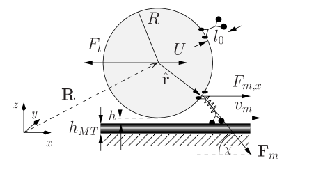
Figure 1: A single sphere of radius $R$ and surface separation $h$ from a planar wall. The translational coordinates $\mathbf{R}$ of the sphere are given relative to a reference frame that is fixed to the wall. The sphere is pulled by one molecular motor that is attached to the surface at position $\hat{{\mathbf{r}}}$ measured with respect to the center of the sphere. The bead is subject to the motor force ${\mathbf{F}}_{m}$ with $x$-component $F_{m,x}$. In addition, an external force $F_{t}$ acts parallel to the filament, typically arising from an optical trap. The force unbalance between $F_{m,x}$ and $F_{t}$ leads to the bead velocity $U$. The motor with resting length $l_{0}$ is firmly attached to the bead and can bind to and unbind from a MT and moves with velocity $v_{m}$. $\chi$ denotes the angle between motor and MT.

In our model the spherical cargo particle is uniformly covered with $N_{tot}$ motor proteins. These molecules are firmly attached to the sphere at their foot domains. Consequently, $N_{tot}$ is a constant in time. The opposite ends of these molecules (their head domains) can reversibly attach to the microtubule (MT), which is modeled as a line of equally spaced binding sites for the motors covering the wall. A motor that is bound to the MT exerts a force and a torque to the cargo particle. If ${\mathbf{r}}_{h}$ and ${\mathbf{r}}_{f}$ are the positions of the head and foot domains of the motor, respectively, then the force by the motor ${\mathbf{F}}_{m}$ is given by:

$${\mathbf{F}}_{m}=\hat{{\mathbf{r}}}_{m}F_{m},\hskip 28.45274ptF_{m}=F(r_{m}),\hskip 28.45274pt\hat{{\mathbf{r}}}_{m}=\frac{{\mathbf{r}}_{h}-{\mathbf{r}}_{f}}{\|{\mathbf{r}}_{h}-{\mathbf{r}}_{f}\|},\hskip 28.45274ptr_{m}=\|{\mathbf{r}}_{h}-{\mathbf{r}}_{f}\|,$$ (4)

where the absolute value $F_{m}$ of the motor force is given by the force extension relation $F(x)$ for the motor protein. Throughout this article we consider two variants of the force extension curve for the polymeric tail of the motor. The harmonic spring model reads

$$F(x)=\kappa(x-l_{0}).$$ (5)

This means, a force is needed for both compression and extension of the motor protein. Actually, it was found that kinesin exhibits a non-linear force extension relation [32], with the spring constant varying between $\kappa=0.2\cdot 10^{-4}$ N/m for small extensions and $\kappa=0.6\cdot 10^{-4}$ N/m for larger extensions [32, 33]. For extensions close to the contour length the molecule becomes infinitely stiff [34]. For small extensions, however, the harmonic approximation works well. Alternatively, we consider the cable model

$$F(x)=\kappa(x-l_{0})\Theta(x-l_{0}),\hskip 28.45274pt\Theta(x)=\left\{\begin{array}[]{l}1,\hskip 28.45274ptx>0\\ 0,\hskip 28.45274pt\mbox{else}\end{array}\right..$$ (8)

In the cable model force is only built up when the motor is extended above its resting length $l_{0}$. In the compression mode, i. e. when the actual motor length is less then the resting length, no force exists. The cable model can be seen as the simplest model for a flexible polymer.

Besides the force each motor attached to the MT also exerts a torque on the cargo particle. With $\hat{{\mathbf{r}}}$ being the position of the motor foot relative to the center of the sphere (cf. Fig. 1), this torque reads

$${\mathbf{T}}_{m}=\hat{{\mathbf{r}}}\times{\mathbf{F}}_{m}.$$ (9)

The combined force/torque vector ${\mathbf{F}}=({\mathbf{F}}_{m},{\mathbf{T}}_{m})^{T}$ enters the Langevin algorithm Eq. (3).

In addition to the firm attachment of the motors to the sphere, each motor can in principle reversibly bind and unbind to the MT. We model these processes as simple Poissonian rate processes in similar a fashion as it is done for modeling of formation and rupture of receptor ligand bonds in cell adhesion (e. g., [22]). The motor head is allowed to rotate freely about its point of fixation on the cargo. The head is therefore located on a spherical shell with radius given by the motor resting length $l_{0}$. However, in contrast to the anchorage point on the cargo particle the head position of the motor is not explicitely resolved by the algorithm. In order to model the binding process we introduce a capture length $r_{0}$. A motor head can then bind to the MT with binding rate $\pi_{ad}$ whenever the spherical shell of radius $l_{0}$ and thickness $r_{0}$ around the motor’s anchorage point has some overlap with a non-occupied binding site on the MT. The MT’s binding sites are identified by the tubulin building block of length $\delta=8$ nm, so we choose $r_{0}=\delta/2$. Note that binding rate and binding range are complementary quantities and that a more detailed modeling of the binding process would have to yield appropriate values for both quantities. If the overlap criterion is fulfilled within a time interval $\Delta t$, the probability for binding $p_{on}$ within this time step is $p_{on}=1-\exp(-\pi_{ad}\Delta t)$. With a standard Monte-Carlo technique it is then decided whether binding occurs or not: a random number $rand$ is drawn from the uniform distribution on the interval $(0,1)$ and in the case $p_{on}>rand$ binding occurs. If the overlap criterion is fulfilled for several binding sites, then using the Monte-Carlo technique it is first decided whether binding occurs and then one of the possible binding sites is randomly chosen.

Parameter	typical value	meaning	reference
$R$	$1~{}\mu$m	bead radius
$\epsilon_{0}$	$1$ s-1	unstressed escape rate	[7]
$\pi_{ad}$	$\mathbf{5}$ s-1	binding rate	[6, 7]
$F_{d}$	3 pN	detachment force	[7, 35]
$\kappa$	$10^{-5}\ldots\mathbf{10^{-4}}\ldots 10^{-3}$ N/m	motor spring constant	[36, 34, 33]
$\delta$	8 nm	kinesin step length	[2]
$v_{0}$	$1~{}\mu$m/s	maximum motor velocity	[7]
$\lambda_{s}^{0}:=v_{0}/\delta$	125 s-1	forward step rate
$r_{0}$	$\delta/2$	capture radius
$F_{s}$	$5\ldots\mathbf{6}\ldots 8$ pN	stall force	[3]
$l_{0}$	50,65,80 nm	(resting) length	[37, 24]
$h_{MT}$	24 nm	microtubule diameter	[25]

Table 1: Parameters used for adhesive motor dynamics. For ambient temperature we use $T=293$ K, for viscosity $\eta=1$ mPa s (if not otherwise stated). If a range is given, then figure in bold face denotes the value used in the numerical simulations.

Each motor bound to the MT can unbind with escape rate $\epsilon$. In single motor experiments it was found that the escape rate increases with increasing motor force [35]. This force dependence can be described by the Bell equation [38, 7]

$$\epsilon=\epsilon_{0}\exp(F_{m}/F_{d}),$$ (10)

with the unstressed escape rate $\epsilon_{0}$ and the detachment force $F_{d}$. Because the details of forced motor unbinding from a filament are not known, here we make the simple assumption that the unbinding pathway is oriented in the direction of the tether. We set $\epsilon=\epsilon_{0}$ whenever the motor is compressed.

The major conceptual difference between a motor connecting a sphere with a MT and a receptor-ligand bond is that a motor can actively step forward from one binding site to the next with step length $\delta$ (the length of the tubulin unit). The mean velocity $v_{0}$ of an unloaded kinesin motor is about $v_{0}=1~{}\mu$m/s depending on ATP concentration [3]. If the motor protein is mechanically loaded with force opposing the walking direction, the motor velocity $v_{m}$ is decreased. For a single kinesin molecule that is attached to a bead on which a trap force $F_{t}$ pulls, the velocity was found experimentally to decrease approximately linearly [39, 3]:

$$v_{m}=v_{0}\left(1-\frac{F_{t}}{F_{s}}\right),\hskip 28.45274pt0<F_{t}<F_{s},$$ (11)

with the stall force $F_{s}$ and the trap force $F_{t}$ acting antiparallel to the walking direction. Different experiments have reported stall forces between 5 and 8 pN. Changes in this range are not essential for our results and therefore we use the intermediate value $F_{b}=6\ pN$. If the force is higher than the stall force, kinesin motors walk backwards with a very low velocity [40], which we will neglect in the following. Finally, for assisting forces, i.e. if the motor is pulled forward, the effect of force is relatively small [41, 40]. In order to derive an expression similar to Eq. (11) for our model, we have to identify the proper term that replaces $F_{t}$ in Eq. (11). First, we rewrite Eq. (11) as $v_{m}=\mu_{m}(F_{s}-F_{t})$, with some internal motor mobility coefficient $\mu_{m}:=v_{0}/F_{s}$. This version of Eq. (11) allows us to interpret the motor head as an over-damped (Stokesian) particle that constantly pulls with the force $F_{s}$ against some external load $F_{t}$ resulting in the effective velocity $v_{m}$. According to Eq. (4) a motor pulls with force ${\mathbf{F}}_{m}$ on the bead, so we can identify the “load” to be $-F_{m,x}$, where $F_{m,x}$ is the $x$-component of ${\mathbf{F}}_{m}$ and the minus sign accounts for Newton’s third law (actio = reactio). Thus, we obtain the following piecewise linear force velocity relation for the single motor (see also Fig. 2):

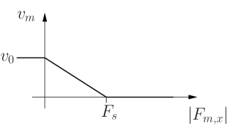
Figure 2: Force velocity relation for a single motor: velocity $v_{m}$ as a function of load $|F_{m,x}|$ according to Eq. (15) with maximum velocity $v_{0}$ and stall force $F_{s}$.

$$v_{m}=v_{0}\left\{\begin{array}[]{ccc}1&\;\;\;\mbox{if}&{\mathbf{F}}_{m}\cdot{\mathbf{e}}_{x}\leq 0\\ 1-\frac{|F_{m,x}|}{F_{s}}&\;\;\;\mbox{if}&0<{\mathbf{F}}_{m}\cdot{\mathbf{e}}_{x}<F_{s},\\ 0&\;\;\;\mbox{if}&{\mathbf{F}}_{m}\cdot{\mathbf{e}}_{x}\geq F_{s}\end{array}\right.$$ (15)

where ${\mathbf{e}}_{x}$ is the walking direction of the motor, see Fig. 1. Thus, if the motor pulls antiparallel to its walking direction on the bead, it walks with its maximum speed $v_{0}$. If it is loaded with force exceeding the stall force $F_{s}$, it stops. For intermediate loadings the velocity decreases linearly with load force. Eq. (15) defines the mean velocity of a motor in the presence of loading force. We note that our algorithm also allows us to implement more complicated force-velocity relations and is not restricted to the piecewise linear force-velocity relation. It is used here because we do not focus on a specific kinesin motor and because it is easy to implement in the computer simulations. In practice the motor walks with discrete steps of length $\delta$. In the algorithm we account for this by defining a step rate $\lambda_{s}:=v_{m}/\delta$. The decision for a step during a time interval $\Delta t$ is then made with the same Monte-Carlo technique used to model the binding and unbinding process of the motor head. A step is rejected if the next binding site is already occupied by another motor (mutual exclusion) [42].

II.3 Bead versus motor friction

In principle, the velocity of a single motor $v_{m}$ pulling the sphere and the component in walking direction of the sphere’s velocity $U$ (see Fig. 1) are not the same. For an external force $F_{t}$ (against walking direction) in the pN range acting on the sphere and $F_{m,x}$ being the motor force in walking direction, the bead velocity $U$ is given by $U=\mu_{xx}^{tt}(F_{m,x}-F_{t})$,. Here, $\mu_{xx}^{tt}$ denotes the corresponding component of the mobility matrix $\mathsf{M}$ of the sphere (cf. Eq. (1)) evaluated at the height of the sphere’s center with super indices $tt$ referring to the translational sector of the matrix and sub indices $xx$ referring to the responses in $x$-direction. On the other hand from Eq. (15) it follows that the motor head moves with velocity $v_{m}=\mu_{m}(F_{s}-F_{m,x})$. Only in the stationary state of motion the two speeds are equal, $U=v_{m}$, and we obtain the force with which the motor pulls (in walking direction) on the bead:

$$F_{m,x}=\frac{\mu^{tt}_{xx}}{\mu_{m}+\mu^{tt}_{xx}}F_{t}+\frac{\mu_{m}}{\mu_{m}+\mu^{tt}_{xx}}F_{s}.$$ (16)

Thus, if the internal friction of the motor is large compared to the viscous friction of the sphere, i. e., $1/\mu_{m}\gg 1/\mu^{tt}_{xx}$, the second term in Eq. (16) can be neglected and one has $F_{m,x}\approx F_{t}$. That means, only the trap force pulls on the motor. If $\mu_{m}\approx\mu^{tt}_{xx}$ both terms in Eq. (16) are of the same order of magnitude. Then, both external load $F_{t}$ and the friction force on the bead will influence the motor velocity. Experimentally, these prediction can be checked in bead assays by varying the viscosities of the medium (e. g., by adding sugar like dextran or Ficoll [43]). Numerically, we can vary $\eta$ in the adhesive motor dynamics algorithm.

When several motors are simultaneously pulling, they can cooperate by sharing the load. Assuming the case that $n$ motors are attached to the MT which equally share the total load, then the force in $x$-direction exerted on the bead is $nF_{m,x}(n)$ with $F_{m,x}$ being again the individual motor force. In the stationary state with $U=v_{m}$ we have (with external load $F_{t}=0$):

$$F_{m,x}(n)=\frac{\mu_{m}}{n\mu_{xx}^{tt}+\mu_{m}}F_{s}.$$ (17)

The mean bead velocity $U(n)$ with $n$ equally pulling motors is $U(n)=n\mu_{xx}^{tt}F_{m,x}(n)$. Thus, in general, the velocity of the beads will increase with increasing number $n$ of pulling motors. However under typical experimental conditions in vitro, where bead movements are probed in aqueous solutions, the internal motor friction $1/\mu_{m}$ dominates over the viscous friction of the bead, $1/\mu_{xx}^{tt}$, and the velocity becomes independent of the number of motors. Only if the bead friction becomes comparable to the internal motor friction, the velocity exhibits an appreciable dependence on the motor number. This dependence can be illustrated by considering the ratio of $U(n)$ and $U(1)$:

$$\frac{U(n)}{U(1)}=\frac{n\mu_{xx}^{tt}+n\mu_{m}}{n\mu_{xx}^{tt}+\mu_{m}}=\frac{n/\mu_{m}+n/\mu_{xx}^{tt}}{n/\mu_{m}+1/\mu_{xx}^{tt}}.$$ (18)

In the opposite limit, $n/\mu_{m}\ll 1/\mu_{xx}^{tt}$, i. e., when the viscous bead friction is very large and dominates over the internal motor friction, Eq. (18), leads to $U(n)\approx nU(1)$, and the bead velocity increases linearly with $n$ [7].

II.4 Vertical forces

We note that, although we are mainly interested in the $x$-component of the motor force ${\mathbf{F}}_{m}$, i.e. the component parallel to the microtubule, which enters the force–velocity relation, the motor force also has a component perpendicular to the microtubule, see Fig. 1. This force component tends to pull the bead towards the microtubule and thus to the surface, whenever the bead is connected to the microtubules by a motor. This force is balanced by the microtubule repelling the bead. Additionally, if the bead touches the filament or the wall, diffusion can only move the bead away from the wall. In case of the full spring model, compressed motors can also contribute a repulsion of the bead from the wall. If viscous friction is strong, the normal component of the force arises mainly from the microtubule. In that case, the distance $h$ between the bead and the microtubule is very small, $\langle h\rangle\approx 0$. For small viscous friction, thermal fluctuations play a major role and lead to non-zero distances between the bead and the microtubule, as discussed further in Sec. III.2.

All parameters used for the adhesive motor dynamics simulations together with typical values are summarized in Tab. 1. For the numerical simulations we non-dimensionalize all quantities using $R$ for the length scale, $1/\epsilon_{0}$ for the time scale and the detachment force $F_{d}$ as force scale.

II.5 Master equation approach

When no external load is applied a motor walks on average a time $1/\epsilon_{0}$ before it detaches and the cargo particle might diffuse away from the MT. When several motors on the cargo can bind to the MT the mean run length dramatically increases as was previously shown with a master equation approach [7]. For the sake of later comparison to our simulations we briefly summarize some of these results in the following.

Let $P_{i}$ be the probability that $i$ motors are simultaneously bound to the MT with $i=0,\ldots,N_{m}$ and $N_{m}$ being the maximum number of motors that can bind to the MT simultaneously. Assuming the system of $N_{m}$ motors is in a stationary state and the total probability of having $i=0,\ldots,N_{m}$ motors bound is conserved then the probability flux from one state to a neighboring state is zero. This means that the probability $P_{i}$ of having $i$ bound motors can be calculated by equating forward and reverse fluxes

$$(N_{m}-i)\pi_{ad}P_{i}=(i+1)\epsilon P_{i+1},\hskip 28.45274pti=0,\ldots,N_{m}-1,$$ (19)

where it is assumed that the escape rate $\epsilon$ is a constant with respect to time. The solution to Eq. (19) is given by

$$P_{i}=\left(\begin{array}[]{c}N_{m}\\ i\end{array}\right)\frac{\epsilon^{N_{m}-i}\pi^{i}}{(\epsilon+\pi)^{N_{m}}},\hskip 28.45274pti=0,\ldots,N_{m}.$$ (22)

The probability that $i$ motors are simultaneously pulling under the condition that at least one motor is pulling is $P_{i}/(1-P_{0})$ for $i=1,\ldots,N_{m}$. Then, the mean number of bound motors ${N}_{b}$ (given that at least one motor is bound) is [7, Eq. [13]]

$${N}_{b}=\sum_{i=1}^{N_{m}}\frac{iP_{i}}{1-P_{0}}=\frac{(\pi_{ad}/\epsilon)\left[1+\pi_{ad}/\epsilon\right]^{N_{m}-1}}{\left[1+\pi_{ad}/\epsilon\right]^{N_{m}}-1}N_{m}.$$ (23)

The effective unbinding rate $\epsilon_{eff}$, i. e., the rate with which the system reaches the unbound state, is determined from $\epsilon_{eff}(1-P_{0})=\pi_{ad}P_{0}$. This quantity can also be identified with the inverse of the mean first passage time for reaching the unbound state, when starting with one motor bound [7]. If the medium viscosity is small, i. e., similar to that of water, and no external force is pulling on the bead, we assume that the velocity of the bead $U$ does not depend on the number of pulling motors. The mean run length, that is the mean distance the cargo is transported by the motors in the case that initially one motor was bound, is then the product of mean velocity $U$ and mean lifetime ($1/\epsilon_{eff}$) [7, Eq. [14]]:

$$\langle\Delta x_{b}\rangle=\frac{U}{\epsilon_{eff}}=\frac{U}{N_{m}\pi_{ad}}\left[\left(1+\frac{\pi_{ad}}{\epsilon}\right)^{N_{m}}-1\right].$$ (24)

For kinesin-like motors at small external load with $\pi_{ad}\gg\epsilon$ this expression can be approximated by $\langle\Delta x_{b}\rangle\approx(U/N_{m}\epsilon)(\pi_{ad}/\epsilon)^{N_{m}-1}$, i. e., the mean run length grows essentially exponentially with $N_{m}$. In the stationary state the bead velocity $U$ and the motor velocity $v_{m}$ are equal. For no external load and small viscous friction on the bead one can approximate $\epsilon\approx\epsilon_{0}$ in Eq. (23) and Eq. (24).

II.6 Mean run length for a spherical cargo particle

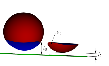
Figure 3: Illustration of the area fraction $a_{b}$ of the sphere (cut and placed besides the sphere) on which motor proteins can reach the MT (thin cylinder). $a_{b}$ depends in a geometrical fashion on the minimum distance $h$ between the sphere and the MT and on the resting length $l_{0}$.

In contrast to the master equation model in which one fixes the maximal number of bound motors $N_{m}$, in the computer simulations only the total number $N_{tot}$ of motors on the spherical cargo particle is fixed. A similar situation arises in experiments where only the total amount of molecular motors on the sphere is measured [14] (but not in experiments with defined multi-motor complexes [16]). If $A_{b}$ is the area on the sphere’s surface that includes all points being less than $l_{0}$ apart from the MT (cf. Fig. 3), we expect on average $n_{b}=N_{tot}a_{b}$ motors to be close enough to the MT for binding, with the reduced area $a_{b}:=A_{b}/(4\pi R^{2})$. While the master equation model assumes a fixed $N_{m}$, in the simulations the maximum number of motors that can simultaneously bind to the MT is a fluctuating quantity about the mean value $n_{b}$. In the simulations the motors are uniformly distributed on the cargo, thus the probability distribution function $P(k)$ for placing $k$ motors inside the above defined area fraction $a_{b}$ is a binomial distribution. As we have $l_{0}\ll R$, $a_{b}$ is small and $P(k)$ is well approximated by the Poissonian probability distribution function

$$P(k,n_{b})=\frac{n_{b}^{k}}{k!}\exp(-n_{b}),\hskip 56.9055ptn_{b}=N_{tot}a_{b}.$$ (25)

Thus, given a fixed number $N_{tot}$ of motors on the sphere the number of motors that are initially in binding range to the MT might be different from run to run. In addition, because of thermal fluctuations and torques that the motors may exert on the cargo particle the relative orientation of the sphere changes during a simulation run. With the change of orientation also the number of motors in binding range to the MT is not a constant quantity during one run.

In order to make simulation results for the mean run length and the mean number of bound motors comparable with the theoretical predictions Eq. (24) and Eq. (23), respectively, we have to average over different $N_{m}$. Neglecting fluctuations in the number of motors that are in binding range to the MT during one simulation run we perform the average with respect to the Poisson distribution, Eq. (25). Averaging the mean walking distance $\langle\Delta x_{b}\rangle(N_{m})$ from Eq. (24) over all $N_{m}$ with weighting factors given by Eq. (25) we obtain the following expression ($n_{b}=a_{b}N_{tot}$):

$$\left.\langle\langle\Delta x_{b}\rangle\rangle_{Poisson}=\sum\limits_{N_{m}=1}^{N_{m,max}}\frac{n_{b}^{N_{m}-1}}{(N_{m}-1)!}\frac{U}{N_{m}\pi_{ad}}\left[\left(1+\frac{\pi_{ad}}{\epsilon_{0}}\right)^{N_{m}}-1\right]\right/\sum\limits_{N_{m}=1}^{N_{m,max}}\frac{n_{b}^{N_{m}-1}}{(N_{m}-1)!}.$$ (26)

We note that during the initialization of each simulation run we place one motor on the lower apex of the sphere and then distribute the other $N_{tot}-1$ motors uniformly over the whole sphere (see appendix B for a detailed description of the procedure). For this reason $P(N_{m}-1,n_{b})$ denotes the probability of having in total $N_{m}$ motors inside the area fraction $a_{b}$. Furthermore, we introduced a cutoff $N_{m,max}$ of maximal possible motors ($N_{tot}$ is obviously an upper limit for $N_{m,max}$). In the limit $N_{m,max}\rightarrow\infty$ we have $\langle\langle\Delta x_{b}\rangle\rangle_{Poisson}=U(e^{\pi_{ad}n_{b}/\epsilon_{0}}-1)/(\pi_{ad}n_{b})$.

In a similar way we can calculate the Poisson-averaged mean number of bound motors $\langle{N}_{b}\rangle_{Poisson}$. For this it is important to include the correct weighting factor [44]. From an ensemble of many simulation runs those with larger run length contribute more than those with smaller run length. For $N$ simulation runs the mean number of bound motors is obtained as $\langle{N}_{b}\rangle_{sim}=\sum_{i}t_{i}n(i)/\sum_{i}t_{i}$, where $t_{i}$ is a period of time during which $n(i)$ motors are bound and the sum is over all such periods of time. Assuming the bead velocity $U$ to be a constant, the time periods $t_{i}$ can also be replaced by the run lengths $\Delta x_{b,i}$ during $t_{i}$. Picking out all simulation runs with a fixed $N_{m}$, their contribution to the sum is the mean number of bound motors ${N}_{b}$ times the total run length of beads with given $N_{m}$. The latter is the mean run length $\langle\Delta x_{b}\rangle_{N_{m}}$ times the number of simulation runs with the given $N_{m}$ (for sufficiently large $N$). Clearly, the fraction of runs with given $N_{m}$ is the probability $P(N_{m}-1,n_{b})$ introduced in Eq. (25). Consequently, we obtain again with a truncation of the sum at some $N_{m,max}\leq N_{tot}$

$$\langle{N}_{b}\rangle_{Poisson}=\sum_{N_{m}=1}^{N_{m,max}}\bar{P}(N_{m}){N}_{b}(N_{m})=\frac{\sum_{N_{m}=1}^{N_{m,max}}P(N_{m}-1,n_{b})\langle\Delta x_{b}\rangle_{N_{m}}{N}_{b}(N_{m})}{\sum_{N_{m}=1}^{N_{m,max}}P(N_{m}-1,n_{b})\langle\Delta x_{b}\rangle_{N_{m}}}.$$ (27)

Here we introduced the probability $\bar{P}(n)$ for having $n$ motors in binding range to the MT when picking out some cargo particle from a large ensemble of spheres. Explicitely, this probability is given by

$$\bar{P}(n)=\frac{\frac{U}{\pi_{ad}}((1+\pi_{ad}/\epsilon)^{n}-1)\frac{n_{b}^{n-1}}{n!}e^{-n_{b}}}{\sum_{i=1}^{N_{m,max}}\frac{U}{\pi_{ad}}((1+\pi_{ad}/\epsilon)^{i}-1)\frac{n_{b}^{i-1}}{i!}e^{-n_{b}}}=\frac{((1+\pi_{ad}/\epsilon_{0})^{n}-1)n_{b}^{n-1}/n!}{\sum_{i=1}^{N_{m,max}}((1+\pi_{ad}/\epsilon_{0})^{i}-1)n_{b}^{i-1}/i!}.$$ (28)

II.7 Computer simulations

We use the following procedure for the computer simulations. In each simulation run the sphere is covered with $N_{tot}$ motors. Initially, one motor, located at the lowest point of the sphere, is attached to the microtubule such that the distance of closest approach $h$ between the sphere and the microtubule is given by the resting length of the motor, i. e., $h=l_{0}$. The other $(N_{tot}-1)$ motors are uniformly distributed on the sphere’s surface (cf. Sec. B). When the motor starts walking, it pulls the sphere closer to the MT because there is a $z$-component in the force exerted on the sphere by the motor stalk (which is strained after the first step). Then, other motors can bind to the MT. The system needs some time to reach a stationary state of motion, so initially the motor velocity $v_{m}$ and the bead velocity $U$ are not the same (for reasons of comparison a fixed initial position is necessary; other initial positions have been tested but initialization effects were always visible). In principle a simulation run lasts until no motor is bound. For computational reasons, each run is stopped after $2\cdot 10^{4}$ s (which is rarely reached for the parameters under consideration). For each run quantities like the mean number of bound motors ${N}_{b}$, the walking distance $\Delta x_{b}$ and the mean distance of closest approach $\langle h\rangle$ between sphere and MT are recorded.

III Results

III.1 Single motor simulations

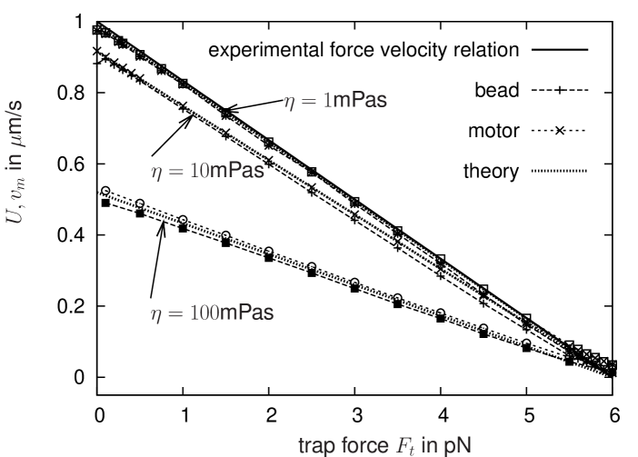
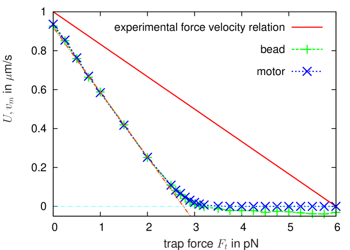
(a)	(b)

Figure 4: (a) Measured force velocity relation of a single motor (with $l_{0}=80$ nm) pulling a sphere of radius $R=1~{}\mu$m for three different viscosities $\eta=1,10,100$ mPa s. Shown is the relation according to Eq. (11), the actual measured force velocity relation of the motor head and the bead center, respectively, and the theoretical prediction according to Eq. (15) and Eq. (16). (b) The measured force velocity relation for $\eta=1$ mPa s is shown where in Eq. (15) not $|F_{m,x}|$ but $\|{\mathbf{F}}_{m}\|$ is used. The dotted line emphasizes the linear decrease of the velocity. The negative velocity of the bead at large $F_{t}$ results from thermal fluctuations. Fluctuations against walking direction increase the escape probability. In case of escape they cannot be compensated by fluctuations in walking direction. (Numerical parameters: $\Delta t=10^{-5}$, number of runs $N=2\cdot 10^{3}-9\cdot 10^{4}$.)

In Sec. II.2 we defined a force-velocity relation for the single motor. In this section we perform simulation runs with a single motor, i. e., $N_{tot}=1$, and measure the effective force velocity relation by tracking the position of the sphere. Inserting Eq. (16) into Eq. (15) provides a prediction for the velocity of a bead subject to one pulling motor and an external trap force $F_{t}$. In Fig. 4a this prediction is shown for three different values of viscosity together with the actual measured velocities during the simulations. More precisely, we measured the mean velocity of the bead and the motor obtained from a large number of simulation runs (to avoid effects resulting from the initial conditions we first allowed the relative position/orientation of bead and motor to “equilibrate” before starting the actual measurement). The mean velocity is then given as the total (summed up over all simulation runs) run length divided by the total walking time. The good agreement between the numerical results and the theoretical predictions provides a favorable test to the algorithm. At $\eta=1$ mPa s (the viscosity of water), friction of the bead has almost no influence on the walking speed. At hundred times larger viscosities, however, bead friction reduces the motor speed to almost half of its maximum value already at zero external load. Although the velocities of the motor and the bead are expected to be equal, Fig. 4a shows that the motor is slightly faster than the bead. This is a result of the discrete steps of the motor and can be considered as a numerical artefact: at the moment the motor steps forward the motor stalk is slightly more stretched (loaded) than before the step, therefore, the escape probability is increased. The result of unbinding at the next time step would then be that the bead moved a distance $\delta$ less than the motor. For loads close to the stall force the observed velocity is slightly larger than the prediction, which is a result of thermal fluctuations of the bead in combination with the stepwise linearity of the force velocity relation: a fluctuation in walking direction slightly reduces the load on the motor, thus increasing the step rate, whereas fluctuations against walking direction lead to zero step rate.

It was observed by Block et al. that vertical forces on the bead (i. e., in $z$-direction) also reduce the velocity of the motor [41]. But the same force that leads to stall when applied antiparallel to the walking direction has a rather weak effect on the motor velocity when applied in $z$-direction. Using the absolute value of the total force of the motor $\|{\mathbf{F}_{m}}\|$ in Eq. (15) instead of its $x$-component $|F_{m,x}|$, we measure a force velocity relation as shown in Fig. 4b. Again, the velocity decreases essentially linearly with applied external force, but stalls already at around $F_{t}\approx F_{s}/2$ because of vertical contributions of the force $\|{\mathbf{F}}_{m}\|$. As the effect of vertical loading reported in Ref. [41] seems to be much weaker than that shown in Fig. 4b, we reject this choice of force velocity relation.

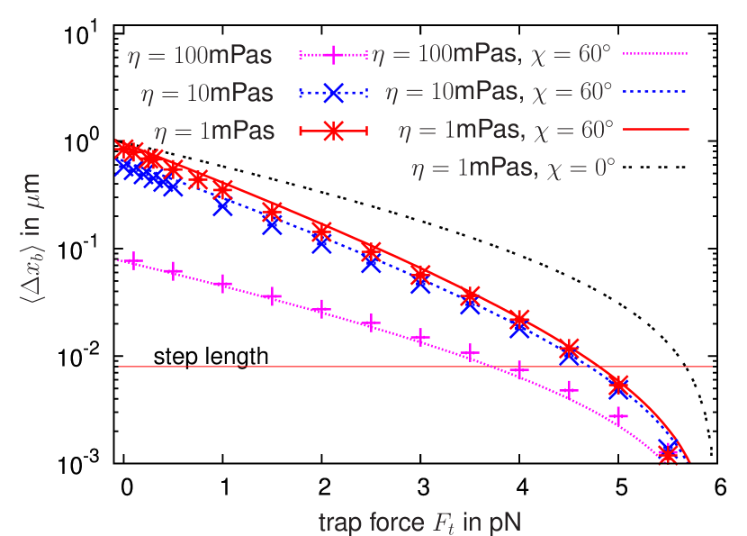
Figure 5: Mean run length $\langle\Delta x_{b}\rangle$ of a bead pulled by a single motor as a function of an external force on the bead $F_{t}$ and for three different viscosities $\eta=1,10,100$ mPa s. The lines give the theoretical predictions according to Eq. (29) assuming an angle of $60^{\circ}$ between the motor and the MT. For comparison also the theoretically predicted $\langle\Delta x_{b}\rangle$-curve for $\chi=0$ is shown (double dotted line).

From the simulations carried out for Fig. 4a we can also obtain the mean run length $\langle\Delta x_{b}\rangle$ for a single motor as a function of external load. The results are shown in Fig. 5. Using Eq. (15) and the Bell equation, Eq. (10), we obtain

$$\langle\Delta x_{b}\rangle=\frac{v_{m}}{\epsilon}=\frac{v_{0}}{\epsilon_{0}}\frac{1-|F_{m,x}|/F_{s}}{\exp(\|{\mathbf{F}}_{m}\|/F_{d})}.$$ (29)

The numerical results shown in Fig. 5 fit very well to the theoretical prediction of Eq. (29) when assuming the angle $\chi$ between the motor and the MT to be $\chi=60^{\circ}$. The angle $\chi$ depends on the bead radius $R$, the resting length $l_{0}$ [45] and the polymer characteristics of the motor protein, e. g., its stiffness $\kappa$.

III.2 Run length for several motors pulling

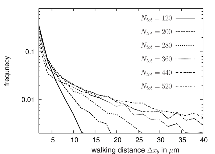
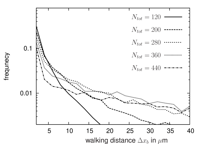
(a)	(b)

Figure 6: Distribution of run lengths $\Delta x_{b}$ in semi-logarithmic scale for different values of motor coverage $N_{tot}$. The motor protein is modeled as a harmonic spring according to Eq. (5). (a) Resting length of the motor protein $l_{0}=50$ nm. (b) Resting length of the motor protein $l_{0}=65$ nm. (Numerical parameters: time step $\Delta t=10^{-5}/\epsilon_{0}$, number of simulation runs $N\approx 10^{4}$.)

We now measure the run length distributions and the mean run length as a function of motor coverage $N_{tot}$. For motors modeled as springs according to Eq. (5) with two different resting lengths $l_{0}=50,65$ nm the run length distributions are shown in Fig. 6a,b. For each value of $N_{tot}$ the run length was measured about $N=10^{4}$ times. The simulations turn out to be very costly, especially for large $N_{tot}$ as the mean run length increases essentially exponentially with the number of pulling motors (cf. Eq. (24)). From Fig. 6 we see that the larger $N_{tot}$, the more probable large run lengths are, resulting in distribution functions that exhibit a flatter and flatter tail upon increasing $N_{tot}$. Fig. 6 nicely shows that the shape of the distributions depends not only on the total number of motors $N_{tot}$ attached to the sphere but also on the resting lengths. Given the same $N_{tot}$ we can see that longer run lengths are more probable for the longer resting length $l_{0}=65$ nm shown in Fig. 6b. This can simply be explained by the fact that the larger the motor proteins, the larger is the area fraction $a_{b}$ introduced in Fig. 3 and therefore the more motors are on average close enough to the microtubule to bind.

Fig. 7a shows the mean run length as a function of $N_{tot}$ as obtained by numerical simulations of the transport process (points with error bars). For the motor stalk three different values of the resting length $l_{0}=50,65,80$ nm are chosen and both the full-spring and the cable model are applied for the force extension relation.

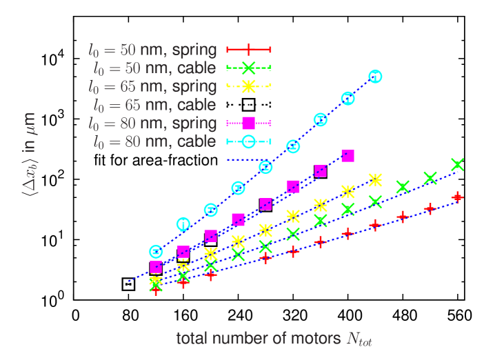
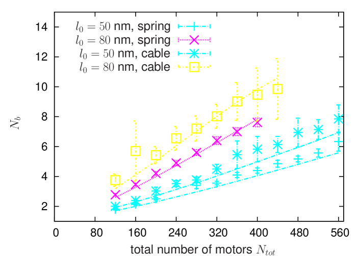
(a)	(b)

Figure 7: (a) Mean run length $\langle\Delta x_{b}\rangle$ (data points with error bars) as a function of motors on the bead $N_{tot}$ obtained from adhesive motor dynamics. The lines are fits of Eq. (26) with respect to the area fraction $a_{b}$. (b) Mean number of bound motors ${N}_{b}$ (data points with error bars). The lines are the values obtained from the Poisson-averaged mean number of bound motors $\langle{N}_{b}\rangle_{Poisson}$ in Eq. (27) using for $a_{b}$ the fit value from (a). (Parameters: $\pi_{ad}=5,\epsilon_{0}=1$, $\lambda_{s}^{0}=125$, $\Delta t=10^{-5}$, $N\sim 10^{4}$.)

Similarly to what we have already seen for the run length distributions in Fig. 6, the larger the resting length $l_{0}$ the more motors can simultaneously bind for given $N_{tot}$, and therefore the larger is the mean run length. Furthermore, Fig. 7a also demonstrates that it makes a clear difference whether the motor stalk behaves like a full harmonic spring or a cable. If the motor protein behaves like a cable (semi-harmonic spring, Eq. (8)) it exhibits force only if it is stretched. The vertical component of this force always pulls the cargo towards the MT. Thus, the mean height between the cargo and the MT (which determines how many motors can bind at maximum) results from the interplay between this force and thermal fluctuations of the bead. In contrast, if the motor also behaves like a harmonic spring when compressed, it once in a while may also push the cargo away from the MT. This results in less motors being close enough to the MT for binding than in the case of the cable-like behavior of the motor stalk. Consequently, given the same $l_{0}$ and $N_{tot}$, the cargo is on average transported longer distances when pulled by “cable-like motors”.

In order to apply the theoretical prediction for the mean run length of a spherical cargo particle, Eq. (26), we need to determine proper values for the three parameters $a_{b}=n_{b}/N_{tot},U,N_{m,max}$. From the simulations we measure the mean velocity of the sphere $U$. It turns out that $U$ is up to 15 % less than the maximum motor velocity $v_{0}$ due to geometrical effects. Depending on the point where the motor is attached on the sphere, some motor steps may result mainly in a slight rotation of the sphere instead of translational motion of the sphere’s center of mass equal to the motor step length $\delta$. For $N_{m,max}$ we choose the overall measured maximum value from all simulation runs for given $N_{tot}$ and polymer model of the motor. Then, we use the remaining parameter, the area fraction $a_{b}$, as a fit parameter to the numerical results. The fits are done using an implementation of the Marquardt-Levenberg algorithm from the Numerical Recipes [46]. The resulting $a_{b}$ values are summarized in Tab. 2. The theoretical curves for those parameter values are shown (dashed lines) in Fig. 7a.

$l_{0}$, motor-model	fit value for $a_{b}$	measured $\langle h\rangle$	$\rightarrow$	$a_{b}(\langle h\rangle)$
$50$nm, spring Eq. (5)	0.00211	7-14 nm	$\rightarrow$	0.0039-0.0034
$50$nm, cable Eq. (8)	0.0026	4-11 nm	$\rightarrow$	0.006-0.0055
$80$nm, spring Eq. (5)	0.00403	8-14 nm	$\rightarrow$	0.0082-0.0076
$80$nm, cable Eq. (8)	0.00518	4-11 nm	$\rightarrow$	0.0085-0.0079

Table 2: Obtained fit values for the area fraction $a_{b}$ for different $l_{0}$ and the two applied polymer models. For comparison the area fraction which is obtained from the measured mean distance $\langle h\rangle$ is also displayed. $\langle h\rangle$ is measured for fixed $N_{tot}$, the left boundary of the provided interval corresponds to the largest $N_{tot}$.

The increase in $a_{b}$ for larger resting length and the cable model is in excellent accordance with the above discussed expectation. An independent estimate of the area fraction can be obtained by measuring the mean distance $\langle h\rangle$ between cargo and MT and calculating the area fraction $a_{b}$ as $a_{b}=a_{b}(\langle h\rangle)$. For comparison those values are also given in Tab. 2. They turn out to be about 60 % larger than the values for $a_{b}$ obtained from the fit. This indicates that the height of the sphere above the MT (and therefore also the area fraction) is a fluctuating quantity that is not strongly peaked around some mean value. Then, because of the non-linear dependence of $a_{b}$ on $h$ we have in general $\langle a_{b}(h)\rangle\neq a_{b}(\langle h\rangle)$.

Fig. 7b shows the mean number of bound motors (the average is obtained over all $N$ simulation runs) as a function of $N_{tot}$ (symbols with error bars). The lines in Fig. 7b are plots of Eq. (27) using the same parameters as for the correspondig lines in Fig. 7a. One recognizes that again the theoretical prediction and the measured values match quite well. This means that on the level of the mean run length and mean number of bound motors the Poission average that was introduced in Sec. II.6 works quite well, even though the number of motors that are in range to the MT is not a constant during one simulation run (cf. Sec. III.3). The large error bars for the cable model data in comparison to the spring model results partly from a poorer statistics (for the $l_{0}=80$ nm cable simulations the number of runs is in the range of some hundreds only). In addition, for cable-like motors the fluctuations in the area fraction $a_{b}$ are much larger than for spring-like motors as repulsive spring forces stabilize the distance between the sphere and the MT. Therefore, the width of the distribution density of the number of bound motors is larger for the cable model than for the spring model. Fig. 7b also shows that for a bead radius of 1 $\mu$m, around 80 motors have to be attached to the bead, otherwise binding and motor stepping become unstable because there are less than two motors left in the binding range.

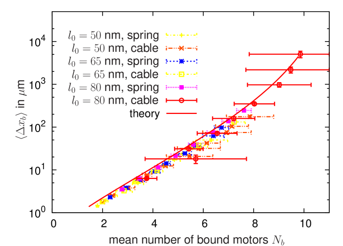
Figure 8: Combination of data from Fig. 7a,b for the resting lengths $l_{0}=50,65,80$ nm. $\langle\Delta x_{b}\rangle$ is shown as a function of ${N}_{b}$. For the dashed line (theory) Eq. (26) and Eq. (27) were combined with a truncation of the sums at $N_{m,max}=18$. (Parameters: $\pi_{ad}=5$ s, $\epsilon_{0}=1$ s, $\lambda_{s}^{0}=125$ s, $\Delta t=10^{-5}/\epsilon_{0}$, $N\sim 10^{4}$.)

In Fig. 8 the simulation results of Fig. 7a,b are combined into one plot. Here we show the measured mean run length $\langle\Delta x_{b}\rangle$ as a function of the mean number of bound motors ${N}_{b}$. All curves collapse on one master curve that can be parametrized by $n_{b}=a_{b}N_{tot}$, i. e., the product of the fit parameter $a_{b}$ and the total number of motors on the sphere. The fact that all data points turn out to lie on one master curve again demonstrates the good applicability of the theoretical predictions to the simulation results. The curve shown in Fig. 8 has a positive curvature in the semi-logarithmic plot. This turns out to be an effect of the finite truncation of the sums in Eq. (26) and Eq. (27).

III.3 Distribution of motors in binding range

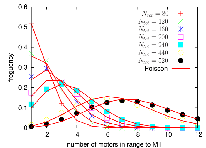
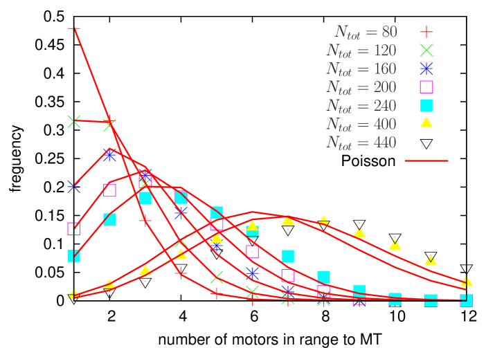
(a)	(b)

Figure 9: Histograms for the number of motors that are in binding range to the MT. Symbols refer to simulation results for different values of the total number of motors on the sphere $N_{tot}$. Lines are Poisson distributions with mean value that is propotional to $N_{tot}$. (a) Resting length $l_{0}=50$ nm, spring model, Eq. (5). (b) Resting length $l_{0}=50$ nm, cable model, Eq. (8). (Parameters: $\pi_{ad}=5,\epsilon_{0}=1$, $\lambda_{s}^{0}=125$, $\Delta t=10^{-5}/\epsilon_{0}$, $N=2\cdot 10^{4}$.)

For the evaluation of the numerical data in Sec. III.2 we assumed that the number of motors that are in binding range to the MT are constant in time and that this number is drawn from a Poisson distribution for every individual run. We now further examine this aspect in order to see to what extend this assumption is fulfilled. First, we measure directly the distribution of the number of motors $n_{MT}$ in binding range to the MT. For this we count $n_{MT}$ at every numerical time step during one simulation run and repeat this for a large ensemble of runs ($N\sim 10^{4}$). Thus, the histograms (i. e., approximately the probability distributions we are looking for) that are obtained in this way for the relative frequency of $n_{MT}$ are not based on the assumption of constant $n_{MT}$ for every single run.

Fig. 9 shows examples of such histograms (symbols) for a series of different values of the total number of motor coverage $N_{tot}$. For Fig. 9a we used the spring model for the motor polymer, Eq. (5), and for Fig. 9b the cable model, Eq. (8). In both cases the resting length of the motor protein is $l_{0}=50$ nm. In addition, Fig. 9 also displays probability distributions (solid lines) that are obtained from the Poission distribution given that at least one motor is in binding range, i. e., $p(n)=\mu^{n}e^{-\mu}/n!(1-e^{-n})$, with mean value $\mu$ given by $\mu=\mu_{0}N_{tot}$ that can be parametrized by some variable $\mu_{0}$. The parameter $\mu_{0}$ was chosen to be 0.015 and 0.0165 for the spring and cable model, respectively, by matching the Poisson distribution to the simulation data. For the spring model (Fig. 9a), the fit is excellent for all values of $N_{tot}$. One must note however that these distributions are not given by Eq. (25) as indicated by the fact that the parameter $\mu_{0}$ is much larger than the area fraction $a_{b}$ determined in the previous section. Instead one needs to account for the correct weighting factors from the different run lengths. If for the moment we consider the number $n_{MT}$ to be a constant during one run, then the distribution Eq. (28) can be considered to be a useful estimate for the data in Fig. 9. Taking the limit $N_{m,max}\rightarrow\infty$ in Eq. (28) we obtain

$$\frac{(a_{b}(1+\pi_{ad}/\epsilon_{0}))^{n_{MT}}-a_{b}^{n_{MT}}}{e^{a_{b}\pi_{ad}/\epsilon_{0}}-1}\frac{e^{-a_{b}}}{{n_{MT}}!}\approx\frac{b^{n_{MT}}}{{n_{MT}}!}e^{-b},$$ (30)

with $b=a_{b}(1+\pi_{ad}/\epsilon_{0})$. Thus, the result is approximately—except for very small $n_{MT}=1,2$—again a Poisson distribution with parameter $b$. With $\pi_{ad}/\epsilon_{0}=5$ and $a_{b}=0.0021$ from Tab. 2 we get $b=0.013$ which is very close to the value $\mu_{0}=0.015$ used in Fig. 9a.

For the cable model (Fig. 9b), the Poisson fit using a single value for $\mu_{0}$ works well only for the smaller values of $N_{tot}$. For large $N_{tot}$ the data points cannot be fitted by a Poisson distribution. It rather turns out that the ratio of mean value and standard deviation becomes less than one in these cases.

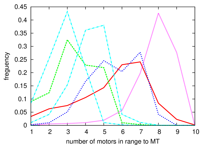
Figure 10: The relative frequencies of the number of motors that are in binding range to the MT during a single run are shown for six different sample runs. For the motor protein the cable model with resting length $l_{0}=50$ nm is used. (Parameters: $N_{tot}=400$, $\pi_{ad}=5$ s, $\epsilon_{0}=1$ s, $\lambda_{s}^{0}=125$ s, $\Delta t=10^{-5}/\epsilon_{0}$).

Finally, we shall note that despite the good agreement between the simulation data and the the estimate from Eq. (30), which was based on the assumption that $n_{MT}$ is constant during one run, $n_{MT}$ is in fact not constant, but a fluctuating quantity. The fluctuations result partly from thermal fluctuations of the height and orientation of the sphere and partly from orientation changes of the sphere that are induced by motor forces. Fig. 10 shows a few sample histograms for the frequency that $n_{MT}$ motors are in binding range to the MT, i.e. either bound to the MT or unbound within the binding range, during a single run. These examples clearly show that $n_{MT}$ takes different values during one run.

III.4 Escape rate distributions

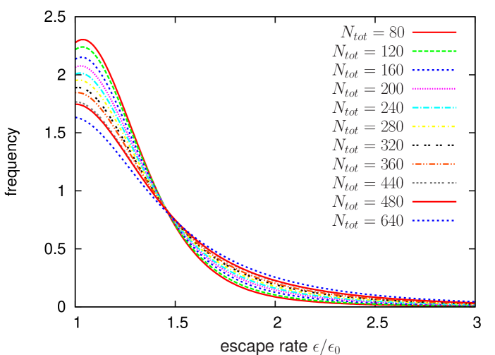
Figure 11: Measured probability distribution density for the escape rate $\epsilon$ given $\epsilon>\epsilon_{0}$. The data was obtained for different values of $N_{tot}$. For the motor proteins the full spring model, Eq. (5), with resing length $l_{0}=50$ nm was used. (Parameters: $\pi_{ad}=5,\epsilon_{0}=1$, $\lambda_{s}^{0}=125$, $\Delta t=10^{-5}/\epsilon_{0}$, $N=2\cdot 10^{4}$.)

Diffusive motion of the cargo sphere directly influences the length of the pulling motor proteins and therefore also the escape rate $\epsilon$. The dependence of the escape rate on the motor length $x$ for $x>l_{0}$ is obtained by inserting the polymer model Eq. (8) and Eq. (5), respectively, into the Bell equation, Eq. (10). For $x\leq l_{0}$ the escape rate is given by $\epsilon=\epsilon_{0}$. For low viscous friction we assume $x$ to be distributed according to a Gaussian distribution. Then, we expect the probability distribution density $\tilde{p}(\epsilon)$ for the escape rate $\epsilon$ to be given by a log-normal distribution density

$$\tilde{p}(\epsilon)=\frac{1}{b\epsilon}\exp{\left(\frac{F_{d}^{2}(\ln(\epsilon)-\ln(\bar{\epsilon}))^{2}}{2k_{B}T\kappa^{*}}\right)}.$$ (31)

Here, $\bar{\epsilon}$ denotes the escape rate associated with the mean motor length in the extended state, $\kappa^{*}$ is an effective spring constant that depends, e. g. on the number of pulling motors, and $b$ is a normalization constant that is obtained from the condition

$$\int_{\epsilon_{0}}^{\infty}\tilde{p}(\epsilon)d\epsilon\stackrel{{\scriptstyle!}}{{=}}1.$$

Fig. 11 shows the measured probability density for $\epsilon>\epsilon_{0}$ and different values of $N_{tot}$. It turns out that the log-normal distribution in Eq. (31) matches well to the measured data (not shown). Fitting Eq. (31) to the data for the effective spring constant $\kappa^{*}$ it turns out that $\kappa^{*}$ increases with increasing $N_{tot}$. This makes sense and illustrates that for several motors pulling the motors behave as a parallel cluster of springs.

The agreement of Eq. (31) with the simulation data for the escape rate distributions suggests that the main source of force acting on the motors and increasing the unbinding rate is due to thermal fluctuations of the micron-sized bead. This is different from what has been reported in experiments with nano-scaled two-motor complexes [16]. There it has been argued that the forces between the two motors arising from their stochastic stepping lead to an increased unbinding rate of these motors.

III.5 Cargo transport against high viscous friction

Except for the single motor simulations of Sec. III.1, all simulation data discussed so far were obtained for a viscosity of $1$ mPa s, corresponding to a water-like solution. We mentioned in Sec. II.2 that load sharing between several motors may lead to cooperative effects at high viscous friction. We now analyze this further by performing simulations at viscosities much larger than that of water (i. e., when the viscous friction on the bead is comparable to the internal friction of the motor protein). To do this we need to measure the velocity of the bead depending on the number of pulling motors. Because of the nature of the stochastic process describing the position of the cargo the instantaneous cargo velocity is however not well defined [47]. Therefore, in order to measure the cargo velocity $U$ we have to average over some time interval $\Delta\bar{t}$. If no motors were pulling the velocity distribution density is given by a Gaussian,

$$p(U,\Delta\bar{t})=\sqrt{\frac{\Delta\bar{t}}{4\pi D}}e^{-U^{2}\Delta\bar{t}/4D},$$ (32)

with diffusion constant $D=k_{B}T_{a}\mu_{xx}^{tt}$ (cf. Sec. II.1). Furthermore we assume a constant height of the sphere so that the mobility coefficient $\mu_{xx}^{tt}$ is a constant in time. The width of the distribution density, Eq. (32), is the smaller the larger $\Delta\bar{t}$ is. So in order to suppress fluctuation effects it seems appropriate to average over a large time interval $\Delta\bar{t}$. On the other hand the number of pulling motors changes with time because of binding and unbinding. Thus, in order to measure the velocity given a certain number of motors $\Delta\bar{t}$ should not be too large in order to get enough such events. Here we choose $\Delta\bar{t}=0.02$ s which corresponds to a typical camera resolution of 50 Hz.

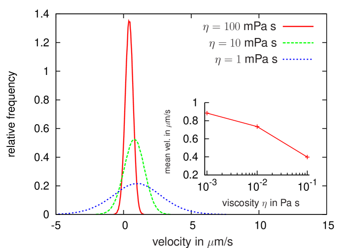
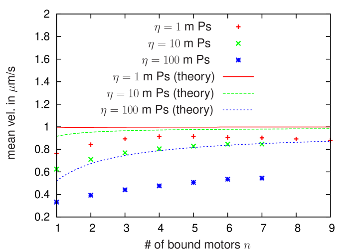
(a)	(b)
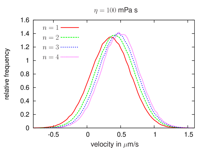
(c)

Figure 12: (a) Propability density of the cargo particle’s velocity $U$ that is obtained by averaging over a time interval of $\Delta\bar{t}=0.02$ s for different values of the viscosity $\eta$. The inset shows the mean velocity as a function of the $\eta$. (b) The mean velocity of the bead given that $n$ motors are simultaneously pulling is plotted as a function of $n$ (symbols). For comparison the theoretical expectation according to Eq. (18) is plotted, too (lines). (c) For high viscosity $\eta=100$ mPas the conditional velocity distribution density given that a certain number of motors is pulling is plotted. (The full harmonic spring model was used; parameters: $l_{0}=80$ nm, $N_{tot}=200$, numerical time step $\Delta t=10^{-5}$, other parameters as in Tab. 1.)

Fig. 12a shows the measured velocity distributions for three different values of the viscosity, $\eta=1,10,100$ mPa s. In the inset of Fig. 12a the mean velocity is plotted as a function of the viscosity. It turns out that shifting the distribution Eq. (32) by the corresponding mean velocity, the single peaked function $p(U,\Delta\bar{t})$ fits qualitatively well to the distribution shown in Fig. 12a, especially the dependence of the width of the distributions on $\eta$ is correctly predicted by Eq. (32). Also a decrease of the mean velocity of the cargo particle is observed with increasing viscosity resulting from the increased frictional load. It must be emphasized that only a single peak is observed in Fig. 12a, even though the bead velocity is expected to depend on the number of pulling motors, which should lead to multiple distinct peaks [7]. One reason that we do not observe multiple peaks is the small value of the time interval $\Delta\bar{t}$, which leads to broad peaks with a peak width governed by diffusion of the bead (cf. Eq. (32)) and thus makes it impossible to separate different peaks. Using larger values of $\Delta\bar{t}$ leads to smaller peak widths, but also to poorer statistics as less measurement points are obtained, so that again distinct peaks cannot be resolved. Even if we do not use a constant time interval, but average over the variable time intervals between two subsequent changes in the number of bound motors [9], distinct peaks are very hard to separate (not shown). This does however not mean that the bead velocity is independent of the number of pulling motors. Indeed if we plot the conditional velocity distribution calculated over all intervals in which the bead is pulled by a certain fixed number of motors, we see a clear shift in the average velocity (Fig. 12c). This shift is however masked by the width of the distributions in Fig. 12a.

In Fig. 12b the average of all measured velocities given that exactly $n$ motors are pulling is plotted as a function of $n$, again for the three different viscosities $\eta=1,10,100$ mPa s. For $\eta=1$ mPa s the viscous friction for the bead is about $1/\mu_{xx}^{tt}\approx 5\cdot 10^{-8}$ Ns/m. The internal friction of the motor is $1/\mu_{m}=F_{s}/v_{0}\approx 6\cdot 10^{-6}$ Ns/m, i. e., about two orders of magnitude larger than $1/\mu_{xx}^{tt}$. According to the analysis at the end of Sec. II.2 we therefore expect that the mean velocity is independent of $n$ if all motors equally share the load. The numerical data in Fig. 12b shows that the mean velocity exhibits a weak dependence on $n$ with a maximum at about $n=4,5$. At the higher viscosities the numerical results show that the mean bead velocity increases with increasing $n$, which indicates that the motors share the load. The simulation data however deviate clearly from the estimate given by Eq. (18), which is indicated by the lines in Fig. 12b. This discrepancy indicates that the load is not shared equally among the motors or that only a subset of the bound motors are actually pulling the bead. Besides geometrical effects one reason why this is the case is that the escape rate $\epsilon_{0}$ is rather high and at high frictional load is even further increased making the lifetimes of motors in the pull state rather short. Then, if a new motor binds to the MT often another motor detaches already before a stationary state is reached in which all the motors equally share the load.

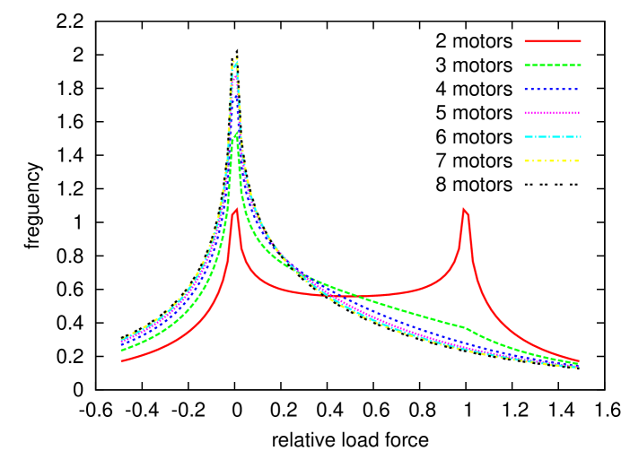
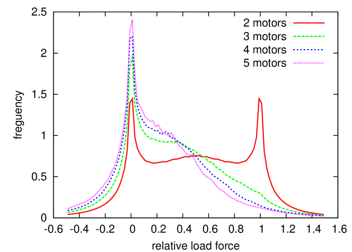
(a)	(b)
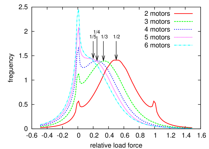
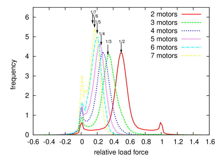
(c)	(d)

Figure 13: Frequencies of the motor forces in walking direction relative to the total load force on the cargo particle for different numbers of pulling motors. (a) Viscosity $\eta=1$ mPa s, escape rate $\epsilon_{0}=1$ s^-1. (b) $\eta=100$ mPa s, $\epsilon_{0}=1$ s^-1. (c) $\eta=100$ mPa s, $\epsilon_{0}=0.1$ s^-1. (d) $\eta=1000$ mPa s, $\epsilon_{0}=0.1$ s^-1. For the other parameters the same values as in Fig. 12 were used.

In order to investigate the last point in more detail we consider explicitely how the force is typically distributed among the pulling motors. For this we count the number $n$ of motors attached at each numerical time step and measure the force experienced by each motor in the direction along the microtubule. For a given number $n$, $n$ such motor forces can be measured, $F_{m,x}^{(i)},i=1,\ldots,n$. To suppress effects from fluctuations in the overall load we then calculate the reduced forces $f_{n}:=F_{m,x}^{(i)}/\sum_{i=1}^{n}F_{m,x}^{(i)}$. Given the histograms for these quantities measured over many time steps and simulation runs we obtain an approximation for the probability distribution density of the relative load of the motors. Fig. 13 shows results for such histograms obtained at different viscosities and two different values of the unstressed escape rate $\epsilon_{0}$. Fig. 13a shows the results for $\eta=1$ mPa s and $\epsilon_{0}=1$ s^-1. One can see some symmetries that result from the definition of the reduced forces. This is especially emphasized for the case of $n=2$ pulling motors. The distribution density of the reduced forces has a mirror symmetry about the value $f_{2}=0.5$. Besides this artefact it turns out that for $n>2$ the distribution densities are strongly peaked at zero force. Thus, for low viscous friction the overall load results mainly from fluctuations. Such loads are typically experienced by a single motor only, whereas the remaining motors are more or less un-stretched. In Fig. 13b the viscosity is 100 times larger than that of water which causes an appreciable load on the pulling motors. However, load sharing effects are hardly visible except for the maxima around $f_{2}=1/2$ and $f_{3}=1/3$, which are rather broad and thus hard to resolve. On the other hand there is still a strongly peaked maximum at $f_{n}=0$. This somewhat surprising observation is due to the rather high escape rate, which is even increased by the load force (cf. Eq. (10)). Therefore, the binding time of the motors is shortend. On the other hand motors that bind to the MT are initially unstressed (i. e., carry zero load) in our model. Thus they always contribute to the $f_{n}=0$ peak and may already escape from the MT before the load is shared equally by all pulling motors. When the escape rate is reduced to $\epsilon_{0}=0.1$ s^-1 as done for Fig. 13c,d clearly visible maxima around $f_{n}=1/n$ appear in the histograms that indicate that the load is equally shared by the active motors. In Fig. 13d where we used the extremely high value of $10^{3}$ mPa s for the viscosity, these peaks are very pronounced. The arrows in Fig. 13c,d indicate the relative force values $1/i,i=2,3,\ldots$. It turns out that the peaks are not exactly located at these values which is again due to the binding and unbinding process of the motors.

In summary, we found that at high loads the pulling motors tend to arrange in such a way that the total load is equally shared amongst them. However, for typical escape rate values of kinesin-like motors this process often takes more time than the lifetime of a state of a certain number of motors bound to the MT lasts, thus preventing cooperativity in the sense of equal load sharing.

IV Discussion and Outlook

The main purpose of this paper is to introduce a novel algorithm called adhesive motor dynamics as a means to study the details of motor-mediated cargo transport. Our algorithm is an extension of existing adhesive dynamics algorithms developed to understand the physics of rolling adhesion [22, 26]. Basically our method allows to simulate the motion of a sphere above a wall including hydrodynamic interactions and diffusive motion by numerically integrating the Langevin equation, Eq. (3). In addition, motor-specific reactions such as binding to the microtubule and stepping are modeled as Poisson processes and then translated into algorithmic rules. The parameters and properties by which the motors are modeled are based on results of single-molecule experiments with conventional kinesin. A first favorable test for the algorithm was provided by measuring the force velocity–relation at different viscosities and external load forces and by comparing the results to the input data as done in Sec. III.1.

Next we measured the run length and the mean number of bound motors as a function of the total number $N_{tot}$ of motors attached to the sphere. The same quantities have been previously calculated based on a one-step master equation model [7]. However, this has been done as a function of a fixed number of motors that are in binding range to the microtubule. In practise and also in our simulations, this quantity varies in time. In Sec. II.6 we Poisson-averaged the theoretical predictions thus rendering it possible to compare theory and simulation results. Using the area fraction on the cargo from which the microtubule is in binding range for the motors as a fit parameter, we found good agreement between theory and simulations for both the mean run length and the mean number of bound motors. Note that the latter one cannot be measured in typical bead assay experiments.

We also determined the mean separation height between cargo and microtubule and found $\langle h\rangle=4-14$ nm. Modeling the motor stalk as a cable resulted in smaller distances than using a full spring model for the motor stalk. A recent experimental study using fluorescence interference contrast microscopy found that kinesin holds its cargo about 17 nm away from the MT [37]. Our smaller distance probably results from neglecting any kind of volume extension (except binding site occupation) of the motor protein, the simplified force extension relation applied to model the stalk behavior, and neglecting electrostatic repulsions. These effects, however, could easily be included into our algorithm, e. g., by using hard core interactions that account for the finite volume of the motor protein segments.

In Sec. III.3 we explicitely demonstrated that the theoretical assumption of having a fixed number of motors in binding range during one walk is not justified (cf. Fig. 10). Nevertheless the theoretical results agree well with the simulations. This might be explainable by the observation that averaged over many runs the distribution of motors in binding range appears to be Poissonian (cf. Fig. 9). Thus, on the one hand fast fluctuations in the number of motors in binding range around some mean value are not visible. On the other hand periods in which this number fluctuates around the same mean value can be treated as a complete run. Thus, averaging over these smaller runs (i. e., which end after the sphere was e. g. rotated visibly and not after the last motor unbinds) has the same effect as averaging over complete runs (i. e., which end after the last motor unbinds).

An interesting question is to what extend several motors can cooperate by sharing load. We have addressed this question for the case of several motors pulling a cargo particle against high viscous friction. One of the advantages of our algorithm is that we can measure the velocity of the bead and at the same time also the number of simultaneously pulling motors. Thus, in Sec. III.5 we tried to check whether the explanation of Ref. [9] is correct also under the assumptions of our model, especially for the parameter values given in Tab. 1. Our simulations show that the speed of the cargo increases with the number of pulling motors for high viscous friction, in agreement with experimental results [48]. Our simulations however show pronounced deviations from the quantitative predictions based on the assumption that the load is shared equally among the bound motors. Furthermore, as the average life time of a state with a certain number of pulling motors is rather short the different velocities expected for different numbers of instantaneously pulling motors were smeared out by diffusion. Similarly when directly measuring how the total load force is distributed to the different motors pulling, no equal load sharing could be observed for the escape rate of about 1 s^-1. We observed equal load sharing only when we used a ten-fold smaller escape rate, in order to increase the life time of the motors in the bound state.

Another interesting question in this context is whether the velocity distribution exhibits several maxima if the cargo is pulled against a viscous load, as observed in several experiments in vivo [9, 49]. For example, Hill et al. [9] found that vesicle in neurites move with constant velocity for some period of time and then switch to another constant velocity in a step-like fashion. The distribution of velocities (measured over time intervals of the order of 1 s) was found to have peaked at integer multiples of the minimal observed velocity. These peaks were interpreted as corresponding to different numbers of simultaneously pulling motors, which equally share the visoelastic load excerted by the cytoplasm [9] (cf. also Eq. (18)). Indeed, both an earlier model for motor cooperation [7] and our present description predict that equal sharing of a large viscous load leads to such a velocity distribution. In our simulations, we could however not resolve multiple peaks, presumably because the peaks are too broad to be resolved. The latter results from a combination of the way how we measure the velocity and from the fast dynamics of motor unbinding as discussed in Sec. III.5.

As already mentioned above, the framework of our method is rather general. Therefore various model variations can be easily implemented and probed in simulations. Here, for example we modeled the motor stalk by two versions of a simple harmonic spring: the cable model, which represents a molecule with an intrinsic hinge, and the spring model. More advanced force–extension relations could easily be incorporate in Eq. (4) in order to probe the influence of more realistic polymer models on the transport process. Similarly, the force dependence in unbinding from the microtubule and stepping can be altered to explore the impact onto macroscopic observables like the mean run length or the speed of the cargo. Furthermore, the algorithm could easily be adapted to study beads to which clusters of motors or defined motor complexes (such as those in ref. [16]) are attached. Thus, the algorithm described in this paper can be regarded as a link between purely theoretical models and data from in vitro experiments.

Another interesting question for future applications of our method is how cargo transport works against some external shear flow. Since our model is based on a hydrodynamic description, flow can easily be included in the dynamics of our model. For these studies the Langevin-equation, Eq. (1), has to be extended by additional terms accounting for the effect of an incident shear flow [28, 23]. Then, two opposing effects exist characterized by the step rate and the strength of the shear flow, respectively. Their interplay together with the rates for binding and unbinding $\pi_{ad}$ and $\epsilon$, respectively, determine whether the cargo moves in walking direction or in flow direction. Experimentally, such a setup might provide interesting perspectives for biomimetic transport in microfluidic devices.

Appendix A Adhesive motor dynamics

The Langevin equation, Eq. (3), and the motor dynamics rules explained in Sec. II.2 are connected by the following algorithmic rules that apply in each time step $\Delta t$:

• The sphere’s position and orientation is updated according to Eq. (3) (for an explicit description see Ref. [26]).

• The positions where the motors are attached to the sphere in the flow chamber coordinate system are calculated.

• For each motor that is bound to the MT its load force is calculated. Then stepping is checked according to the stepping rate derived from Eq. (15). If the motor steps forward the load force is again calculated as motor length/direction has changed.

• For each motor that is not bound to the MT binding is checked according to the procedure explained in the main text (Sec. II.2).

• For each active motor (i. e., bound to the MT), the contribution to ${\mathbf{F}}^{D}$ is calculated.

• Each motor that is bound to the MT can unbind with escape rate $\epsilon$ given by the Bell equation, Eq. (10).

A motor that escaped from the MT in one time step can rebind to the MT in the next time step according to rule (iv). The same Monte-Carlo technique that is explained in the main text (Sec. II.2) to decide whether binding occurs or not is also used for the decission on stepping and unbinding. For the pseudo random number generator we used an implementation of the Mersenne Twister [50].

Appendix B Motor distribution algorithm

Initially the center of the sphere is located at position $(0,0,R+l_{0}+h_{MT})$ directly above a microtubule binding site (cf. Fig. 1). The first motor that is distributed is initially fixed at position $(0,0,l_{0}+h_{MT})$ (relative to the chamber coordinate system) with its tail. The head is bound to the microtubule at $(0,0,h_{MT})$. Thus the initial distance between the motor and the microtubule is given by the motor resting length $l_{0}$. For the distribution of the other $N_{tot}-1$ motors on the sphere we use an hard disk overlap algorithm similarly to the one that was described in Ref. [22]. For each of these motors two random variables are chosen $r_{1}$ from the uniform distribution on $(0,2\pi)$ and $r_{2}$ from the uniform distribution on $(0,1)$, respectively. Then, the motor is located on the sphere’s surface at the spherical coordinates $(r_{1},\arccos(1-2r_{2}))$ and possible overlap to already distributed motors is checked. If no other motor is located within a ball of radius $0.1l_{0}$ around the just distributed motor, then its position is kept, otherwise a new pair of random coordinates are drawn until no overlap with other motors exists.

References

- [1] J. Howard. Mechanics of motor proteins and the cytoskeleton. Sinauer Associates, Sunderland, Massachusetts, 2001.
- [2] D. L. Coy, M. Wagenbach, and J. Howard. Kinesin Takes One 8-nm Step for Each ATP That It Hydrolyzes. The Journal of Biological Chemistry, 274(6):3667–3671, 1999.
- [3] K. Visscher, M. J. Schnitzer, and S. M. Block. Single kinesin molecules studied with a molecular force clamp. Nature, 400:184–189, 1999.
- [4] S. P. Gross, M. Vershinin, and G. T. Shubeita. Cargo transport: two motors are sometimes better than one. Current biology, 17(12):R478–R486, June 2007.
- [5] G. Koster, M. van Duijn, B. Hofs, and M. Dogterom. Membrane tube formation from giant vesicles by dynamic association of motor proteins. PNAS, 100:15583–15588, 2003.
- [6] C. Leduc, O. Campas, K. B. Zeldovich, A. Roux, P. Jolimaitre, L. Bourel-Bonnet, B. Goud, J.-F. Joanny, P. Bassereau, and J. Prost. Cooperative extraction of membrane nanotubes by molecular motors. PNAS, 101:17096–17101, 2004.
- [7] S. Klumpp and R. Lipowsky. Cooperative cargo transport by several molecular motors. PNAS, 102(48):17284–17289, 2005.
- [8] L. S. Goldstein and Z. Yang. Microtubule-based transport systems in neurons: the roles of kinesins and dyneins. Annual review of neuroscience, 23:39–71, 2000.
- [9] D. B. Hill, M. J. Plaza, K. Bonin, and G. Holzwarth. Fast vesicle transport in PC12 neurites: velocities and forces. European Biophysics Journal, 33:623–632, 2004.
- [10] S. P. Gross. Hither and yon: A review of bi-directional microtubule-based transport. Phys. Biol., 1:R1–R11, 2004.
- [11] Melanie J. I. Müller, Stefan Klumpp, and Reinhard Lipowsky. Tug-of-war as a cooperative mechanism for bidirectional cargo transport by molecular motors. Proceedings of the National Academy of Sciences, 105(12):4609–4614, 2008.
- [12] S. M. Block, L. S. Goldstein, and B. J. Schnapp. Bead movement by single kinesin molecules studied with optical tweezers. Nature, 348(6299):348–352, November 1990.
- [13] K. J. Böhm, R. Stracke, P. Mühlig, and E. Unger. Motor protein-driven unidirectional transport of micrometer-sized cargoes across isopolar microtubule arrays. Nanotechnology, 12:238–244, 2001.
- [14] J. Beeg, S. Klumpp, R. Dimova, R. Serral Gracià, E. Unger, and R. Lipowsky. Transport of beads by several kinesin motors. Biophysical Journal, 94:532–541, 2008.
- [15] Michael Vershinin, Brian C. Carter, David S. Razafsky, Stephen J. King, and Steven P. Gross. Multiple-motor based transport and its regulation by tau. Proceedings of the National Academy of Sciences, 104(1):87–92, January 2007.
- [16] A.R. Rogers, J.W. Driver, P.E. Constantinou, D.K. Jamison, and M.R. Diehl. Negative interference dominates collective transport of kinesin motors in the absence of load. Phys. Chem. Chem. Phys., 11:4882–4889, 2009.
- [17] A. Kunwar, M. Vershinin, J. Xu, and S. P. Gross. Stepping, strain gating, and an unexpected force-velocity curve for multiple-motor-based transport. Curr. Biol., 18:1173–1183, 2008.
- [18] D. A Lauffenburger and J. J. Linderman. Receptors. Oxford University Press, 1993.
- [19] T. Erdmann and U. S. Schwarz. Stability of adhesion clusters under constant force. Phys. Rev. Lett., 92:108102, 2004.
- [20] T. Erdmann and U. S. Schwarz. Stochastic dynamics of adhesion clusters under shared constant force and with rebinding. Journal of Chemical Physics, 121(18), 2004.
- [21] T. A. Springer. Traffic signals for lymphocyte recirculation and leukocyte emigration: the multistep paradigm. Cell, 76:301–314, 1994.
- [22] D. A. Hammer and S. M. Apte. Simulation of cell rolling and adhesion on surfaces in shear flow: general results and analysis of selectin-mediated neutrophil adhesion. Biophysical Journal, 63:35–57, 1992.
- [23] C. B. Korn and U. S. Schwarz. Dynamic states of cells adhering in shear flow: From slipping to rolling. Physical Review E, 77(4):041904, 2008.
- [24] M. Schliwa, editor. Molecular Motors. Wiley-VCH, 2003.
- [25] L. Limberis, J. J. Magda, and R. J. Stewart. Polarized Alignment and Surface Immobilization of Microtubules for Kinesin-Powered Nanodevices. Nano Letters, 1(5):277–280, 2001.
- [26] C. B. Korn and U. S. Schwarz. Mean first passage times for bond formation for a Brownian particle in linear shear flow above a wall. Journal of Chemical Physics, 126(9):095103, 2007.
- [27] D. L. Ermak and J. A. McCammon. Brownian dynamics with hydrodynamic interactions. Journal of Chemical Physics, 69(4):1352–1360, 1978.
- [28] J. F. Brady and G. Bossis. Stokesian Dynamics. Ann. Rev. Fluid Mech., 20:111–157, 1988.
- [29] B. Cichocki and R. B. Jones. Image representation of a spherical particle near a hard wall. Physica A, 258:273–302, 1998.
- [30] W. Hortshemke and R. Lefever. Noise-Induced Transitions. Springer-Verlag, 1984.
- [31] G. S. Perkins and R. B. Jones. Hydrodynamic interaction of a spherical-particle with a planar boundary. II. Hard-wall. Physica A, 189:447–477, 1992.
- [32] K. Svoboda, C. F. Schmidt, B. J. Schnapp, and S. M. Block. Direct observation of kinesin stepping by optical trapping interferometry. Nature, 365:721–727, 1993.
- [33] F. Gibbons, J.-F. Chauwin, M. Despósito, and J. V. José. A Dynamical Model of Kinesin-Microtubule Motility Assays. Biophysical Journal, 80:2515–2526, 2001.
- [34] T. Duke and S. Leibler. Motor Protein Mechanics: A Stochastic Model with Minimal Mechanochemical Coupling. Biophysical Journal, 71:1235–1247, 1996.
- [35] M. J. Schnitzer, K. Visscher, and S. M. Block. Force production by single kinesin motors. Nature Cell Biology, 2:718–723, 2000.
- [36] A. Rohrbach, E.-L. Florin, and E. H. K. Stelzer. Photonic Force Microscopy: Simulation of principles and applications. Proceedings of SPIE, 4431:75–86, 2001.
- [37] J. Kerssemakers, J. Howard, H. Hess, and S. Diez. The distance that kinesin-1 holds its cargo from the microtubule surface measured by fluorescence interference contrast microscopy. PNAS, 103(43):15812–15817, 2006.
- [38] G. I. Bell. Models for the Specific Adhesion of Cells to Cells. Science, 200:618–627, 1978.
- [39] K. Svoboda and S. M. Block. Force and velocity measured for single kinesin molecules. Cell, 77(5):773–784, 1994.
- [40] N. J. Carter and R. A. Cross. Mechanics of the kinesin step. Nature, 435(7040):308–312, 2005.
- [41] S. M. Block, C. L. Asbury, J. W. Shaevitz, and M. J. Lang. Probing the kinesin reaction cycle with a 2D optical force clamp. PNAS, 100(5):2351–2356, 2003.
- [42] R. Lipowsky, S. Klumpp, and T. M. Nieuwenhuizen. Random Walks of Cytoskeletal Motors in Open and Closed Compartments. Physical Review Letters, 87(10):108101, 2001.
- [43] S. Chen and T. A. Springer. Selectin receptor-ligand bonds: Formation limited by shear and dissociation governed by the Bell model. PNAS, 98(3):950–955, 2001.
- [44] C. Korn. Stochastic dynamics of cell adhesion in hydrodynamic flow. PhD thesis, Potsdam University, 2007.
- [45] C. L. Asbury, A. N. Fehr, and S. M. Block. Kinesin Moves by an Asymmetric Hand-Over-Hand Mechanism. Science, 302:2130–2134, 2003.
- [46] W. H. Press, S. A. Teukolsky, W. T. Vetterling, and B. P. Flannery. Numerical Recipes in C. Cambridge University Press, second edition, 1994.
- [47] C. W. Gardiner. Handbook of Stochastic Methods. Springer-Verlag, 1985.
- [48] A. J. Hunt, F. Gittes, and J. Howard. The force exerted by a single kinesin molecule against a viscous load. Biophys J, 67(2):766–781, August 1994.
- [49] V. Levi, A. S. Serpinskaya, E. Gratton, and V. Gelfand. Organelle transport along microtubules in xenopus melanophores: evidence for cooperation between multiple motors. Biophysical journal, 90(1):318–327, January 2006.
- [50] M. Matsumoto and T. Nishimura. Mersenne twister: A 623-dimensionally equidistributed uniform pseudorandom number generator. ACM Trans. on Modeling and Computer Simulation, 8(1):3–30, 1998.