Weak Microlensing

Abstract

A nearby star having a near-transit of a galaxy will cause a time-dependent weak lensing of the galaxy. Because the effect is small, we refer to this as weak microlensing. This could provide a useful method to weigh low-mass stars and brown dwarfs. We examine the feasibility of measuring masses in this way and we find that a star causes measurable weak microlensing in a galaxy even at 10 Einstein radii away. Of order one magnitude $I\leq 25$ galaxy comes close enough to one or other of the $\sim 100$ nearest stars per year.

1 Introduction

Gravitational lensing by Galactic stars has come a long way since the low-probability assessment of Einstein (1936). The first detections (Alcock et al. 1993; Aubourg et al. 1993; Udalski et al. 1993) have been followed by $\sim 4000$ more, including a few detections of planets around the main lensing star (e.g., Gould et al. 2006).

Yet despite the now abundant examples of microlensing, accurate measurements of the lensing mass are still rare. The reason is that a microlensing light-curve on its own tells us precisely how long proper motion takes to traverse an Einstein radius, but the physical length $r_{E}$ of the Einstein radius and its angular size $\theta_{E}$ remain unknown. Hence, only a broad statistical statement about the stellar mass can be made in most cases.

Refsdal (1966) anticipated the problem and suggested a way to overcome it: If both stars are directly observable, their relative proper motion would (together with the light curve) supply $\theta_{E}$, while a second observatory in the solar system would provide $r_{E}$. Several related ideas have been forwarded, notably by An et al. (2002), who exploited a combination of caustic-crossing times and finite source size effects to obtain the first microlensing mass measurement. A similar strategy has recently been used by Gould et al. (2009) to measure the mass of a brown dwarf to 10%.

Another possibility is to measure the lensing effect of a star on a galaxy. Paczyński (1996) pointed out that as a Galactic star makes a near-transit of a galaxy, the latter will undergo a small shift in its apparent centroid. For this variety of microlensing to be observable, $\theta_{E}$ needs to be larger than the precision of image centroiding–although it can be below resolution–and proper motions need to be large. Nearby stars are the only realistic prospect, since

$$\theta_{E}\approx 0\mbox{$.\!\!^{\prime\prime}$}09\left(\frac{M/M_{\odot}}{D_{\mathrm{lens}}/{\mathrm{pc}}}\right)^{1/2}$$ (1)

for sources at infinity, and proper motions are $\sim 1^{\prime\prime}$ per year. Microlensing by nearby stars would have none of the degeneracy problems mentioned above; the lens being at known distance, the mass is the only unknown parameter. Moreover, such events are predictable long in advance. The transit may be on the order of a few months allowing for observations of the galaxy both before and during the lensing event. Ideally, the star would not transit directly across the galaxy since the star must be masked out for proper observations of the galaxy.

Paczyński (1996) suggested that microlensing centroid shifts could be used to measure down to masses of nearby brown dwarfs. In this paper, we suggest a refinement of Paczyński’s idea which could make it much more effective. Rather than just the galaxy centroid shift, the whole weakly-lensed image of the galaxy could be exploited to infer the lensing mass. We develop a technique to extract the weak-lensing effects and estimate the mass of the star.

2 A fitting method

Consider a star with Einstein radius $\theta_{E}$ whose sky position at epoch $t$ is $z_{t}$. Lensing by this star maps a point $\theta$ in the image plane to a point $\phi$ in the source plane such that

$$\phi=\theta-\theta^{2}_{E}\frac{(\theta-z_{t})}{|\theta-z_{t}|^{2}}$$ (2)

where $z_{t},\theta,\phi$ are two-dimensional vectors.

Next, we consider a galaxy whose unlensed brightness distribution $S$ is expanded in terms of basis functions $B^{n}(\theta)$ as

$$S(\theta)=\sum_{n}a^{n}B^{n}(\theta)$$ (3)

where $a^{n}$ are the expansion coefficients. In the presence of lensing, the brightness distribution of the galaxy will be

$$S_{t}(\theta)=\sum_{n}a^{n}B^{n}(\phi(\theta,z_{t},\theta_{E}))\quad,$$ (4)

where $S$ now has a time dependence due to the position of the star $z_{t}$. Since lensing conserves surface brightness, the lensed surface brightness at $\theta$ equals the unlensed surface brightness at $\phi$.

Pixelating the image plane, we write the pixel-wise brightness distribution as

$$D_{t,ij}\equiv\sum_{n}a^{n}L^{n}_{t,ij}$$ (5)

where $L^{n}_{t,ij}$ represents a lensed and pixelated basis function

$$L^{n}_{t,ij}\equiv B^{n}(\phi(\theta_{ij},z_{t},\theta_{E}))\quad.$$ (6)

The expression in Equation 5 is our model for the lensed brightness distribution. If the observed distribution is $d_{t,ij}$ then the likelihood is

$$\mathcal{L}(a^{n},\theta_{E})\propto\prod_{t,ij}\exp\big{[}{\textstyle-\frac{1}{2}}\,\sigma^{-2}_{t,ij}\,(d_{t,ij}-D_{t,ij})^{2}\big{]}$$ (7)

where $\sigma_{t,ij}$ is the pixel-wise noise, which we assume is Gaussian. The model has a complicated dependence on $\theta_{E}$, but only a linear dependence on the expansion coefficients $a^{n}$. Since we are not especially interested in the $a^{n}$, we marginalise them out by standard methods (for example, chapter 5 of Saha 2003). The marginalised likelihood is given by

$$2\ln\mathcal{L}(\theta_{E})=\ln|\det C|+\sum_{mn}P_{m}P_{n}C_{mn}-\sum_{t,ij}\sigma^{-2}_{t,ij}\,d^{2}_{t,ij}\quad.$$ (8)

Here

$$P_{n}\equiv\sum_{t,ij}\sigma^{-2}_{t,ij}\,d_{t,ij}\,L^{n}_{t,ij}$$ (9)

represents a kind of projection of the data on the model, while

$$C^{-1}_{mn}\equiv\sum_{t,ij}\sigma^{-2}_{t,ij}\,L^{m}_{t,ij}\,L^{n}_{t,ij}$$ (10)

is the inverse covariance matrix. We can relate $\mathcal{L}(\theta_{E}$) to an effective $\chi^{2}$ as just

$$\mathcal{L}(\theta_{E})=\exp(-\chi^{2}/2)\quad.$$ (11)

We are now prepared to estimate the mass of a star by its lensing effect on a background galaxy. Given the pixel-wise brightness $d_{t,ij}$ and noise level $\sigma_{t,ij}$, we simply need to calculate the effective $\chi^{2}$ and minimize with respect to $\theta_{E}$.

As an aside, $|\det C|$ in Equation 8 will typically overflow floating-point arithmetic, while $\ln|\det C|$ will fit quite nicely. Hence we compute an alternative form, namely, $\ln|\det C|=\sum\ln\lambda_{n}$, where $\lambda_{n}$ is the $n$th eigenvalue of $C$.

3 Simulated Observations

We tested the above scheme using simulated data, focusing specifically on the dependence on four quantities: the actual Einstein radius of the star $\theta_{E,\mathrm{true}}$, the closest approach or impact parameter $p$, the number of observed epochs (or $t$ values) $N_{\mathrm{obs}}$, and the total number of photons collected $\gamma_{\mathrm{tot}}$. The values are summarized in Table 1. The full matrix of these parameters was tested, giving a total of 500 simulated observational programs.

$\gamma_{\mathrm{tot}}$	$\frac{1}{2}$,1,3,7,12	$\times 10^{6}$
$N_{\mathrm{obs}}$	$2,3,4,5$
$\theta_{E,\mathrm{true}}$	$10,20,30,40,50$	[milliarcsec]
$p$	0.08, 0.126, 0.232, 0.454, 0.903	[arcsec]

Table 1: Parameters used for simulated observations: $\gamma_{\mathrm{tot}}$ is the total number of photons over all observation epochs (including one unlensed observation), $N_{\mathrm{obs}}$ is the number of epochs, $\theta_{E,\mathrm{true}}$ is the Einstein radius we wish to recover, and $p$ is the closest approach of the star on the sky plane to the background galaxy.

For the exact form of the unlensed surface brightness in Equation 3 we chose

$$S(\theta)=\exp\left(-7.67\left[\sqrt{(\theta/R_{e})^{2}+R_{c}^{2}}\right]^{1/4}\right)$$ (12)

with $R_{e}=1$. This is simply a de Vaucouleurs profile modified by a core radius $R_{c}$ of 2 pixels to mimic the effect of the telescope PSF on a singular cusp.

We then considered $71\times 71$ pixels imaging a patch of sky $2^{\prime\prime}$ on a side and centred on the galaxy. With this resolution each pixel is about $l=0\mbox{$.\!\!^{\prime\prime}$}028$ across, which, for example, would be equivalent to about one pixel per resolution element of the Nasmyth Adaptive Optics System (NAOS) Near-Infrared Imager and Spectrograph (CONICA) camera (Lenzen et al. 2003; Rousset et al. 2003). At a redshift of $z\sim 0.5$, where we expect to find most of our background galaxies, $1^{\prime\prime}$ is about 6 kpc. The corresponding lensed pixelated brightness is

$$S_{t,ij}=S(\phi(\theta_{ij},z_{t},\theta_{E,\mathrm{true}}))\quad.$$ (13)

We normalized this brightness to the total number of photons

$$\sum_{t,ij}S_{t,ij}=\gamma_{\mathrm{tot}},$$ (14)

and thus $\gamma_{\mathrm{tot}}/N_{\mathrm{obs}}$ is the number of photons per image. Considering the normalized $S_{t,ij}$ as the expectation value of the pixel-wise photon count, we then drew the simulated data $d_{t,ij}$ from a Poisson distribution. The noise level $\sigma_{t,ij}$ was taken as $\sqrt{d_{t,ij}}$, which greatly simplifies Equations 8 and 9.

In practice, the star will be masked out during observations. To simulate this, we discarded the pixels within one pixel-width of the star.

As basis functions we chose two-dimensional Hermite functions or shapelets (e.g., Refregier 2003). The scale parameter for the shapelets was set to $\beta=0\mbox{$.\!\!^{\prime\prime}$}2$ and we used $N_{\mathrm{basis}}=20\times 20$ basis functions in all. These settings allow structures as large as $\theta_{\mathrm{max}}=\beta(2\sqrt{N_{\mathrm{basis}}}+1)^{1/2}=1\mbox{$.\!\!^{\prime\prime}$}28$ and as small as $\theta_{\mathrm{min}}=\beta(2\sqrt{N_{\mathrm{basis}}}+1)^{-1/2}=0\mbox{$.\!\!^{\prime\prime}$}03$ to be resolved (Melchior et al. 2007).

For each of the 500 test cases, we considered one epoch $t=0$ with the galaxy unlensed and additional epochs $t>0$ with the star at $z_{t}=(5lt,{-l2^{i}\;|\;i\in[1,\dots,5]})$. The selection of $i$ corresponds to the selection of $p$: A large $p$ implies a large $i$. This choice of position puts the star at the centre of a pixel. Extensive testing has shown a sensitivity to placing stars near pixel edges, whereby recovery of the data is degraded if the star is too close to pixel boundaries.

In Figure 1 we show the effective $\chi^{2}$ as a function of $\theta_{E}$ for one of the simulated data sets. In Figure 2 we show the simulated images, along with the reconstructed and residual images for the best-fit $\theta_{E}$. Examining such plots is a good indicator of potential problems. For example, if too few basis functions are used, a grid-like pattern shows up in the reconstructions and the residual, and recovery of $\theta_{E}$ is very poor.

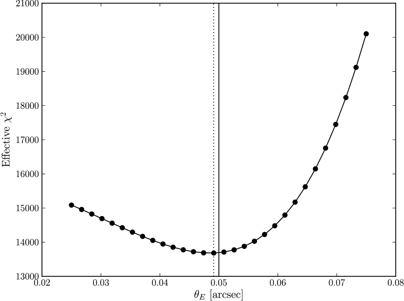
Figure 1: Plot of the effective $\chi^{2}$ as a function of $\theta_{E}$, for a simulated observation program with $N_{\mathrm{obs}}=2$ epochs, total photons $\gamma_{\mathrm{tot}}=3\times 10^{6}$ collected, $\theta_{E,\mathrm{true}}=0\mbox{$.\!\!^{\prime\prime}$}05$ and impact parameter $p=0\mbox{$.\!\!^{\prime\prime}$}126$. The solid vertical line marks $\theta_{E,\mathrm{true}}$ and the dashed line marks the best fit. The formal count of degrees of freedom is $2\;\mathrm{epochs}\times 71^{2}\;\mathrm{pixels}-20^{2}\;\mathrm{basis}\ \mathrm{functions}=9682$, so the effective reduced $\chi^{2}\approx 1.4$. The dependence of the fit on $\theta_{E}$ is non-linear, hence the asymmetric shape of the curve.

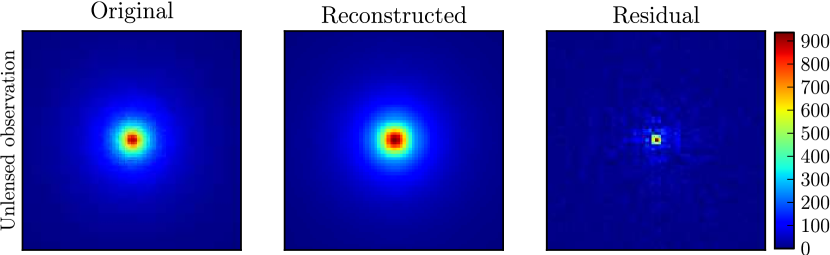
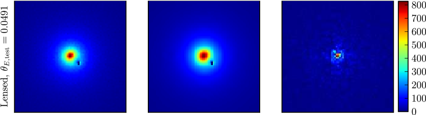
Figure 2: Details of the best-fit $\theta_{E}$ for the simulated observation program of Figure 1. The upper row refers to an unlensed epoch $t=0$ and the lower row to the lensed epoch $t=1$. The left column shows the simulated data $d_{t,ij}$, the middle column shows the best reconstruction $D_{t,ij}$, while the right column is $|d_{t,ij}-D_{t,ij}|$. The scale is in units of photons. The star has been masked out as would be done during an observation.

Figure 3 summarizes the complete suite of 500 simulated observation programs, showing the mass-recovery errors as a function of $\theta_{E,\mathrm{true}},$ $p,$ $\gamma_{\mathrm{tot}}$ and $N_{\mathrm{obs}}$. The following conclusions can be easily read off:

• The mass range of nearby brown dwarfs is accessible, since $\theta_{E}$ down to $0\mbox{$.\!\!^{\prime\prime}$}02$ can be measured with the resolution considered.

• Impact parameters of $p\sim 10\,\theta_{E}$ are small enough, but if $p$ is too small the galaxy can be obscured by the star mask, leading to poor results.

• Of order a million photons from the galaxy are needed, and a few times this are desirable, but it does not matter much whether these are concentrated in two epochs or distributed among several epochs.

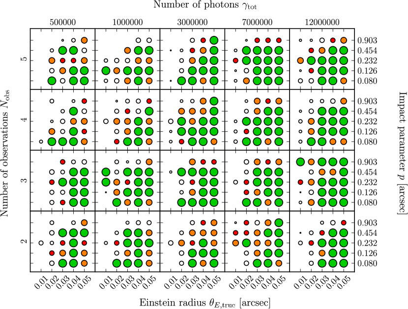
Figure 3: Mass uncertainty as a function of four quantities: $\theta_{E}$, impact parameter $p$, total galaxy photons collected $\gamma_{\mathrm{tot}}$, and the number of epochs $N_{\mathrm{obs}}$. Within each box, $\theta_{E}$ and $p$ are varied at fixed $\gamma_{\mathrm{tot}},N_{\mathrm{obs}}$. The latter two quantities are varied between boxes, as labelled. Circles indicate the error in mass (i.e., in $\theta_{E}^{2}$): Large, green circles denote $<5\%$ error, orange circles 5–11% error, red circles 11-20% error, and small, open circles are used if the mass error was $>20\%$. Missing circles mean that no mass estimate could be made. Of all the tests, 26% have errors less than 5% and 39% have errors less than 11%. Of those tests with filled circles, 52% have errors less than 5% and 79% have errors less than 11%.

4 Event rates

We now consider how likely is it to find a star crossing near a background galaxy. For this analysis we used the Research Consortium on Nearby Stars (RECONS) list of the 100 nearest stellar systems (Henry 2009). The proper motions and estimated masses of the stars in these systems are plotted in Figure 4. In Figure 5 we have plotted the area of sky swept out by Einstein radii per year, or $2\,\mu\theta_{E}$ where $\mu$ is the proper motion.

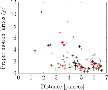
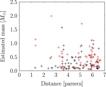
Figure 4: The nearest 100 stellar systems (139 stars) from the RECONS catalogue. Shown are the proper motions (left) and estimated masses (right) for the sample. Systems in red have been excluded from the discussion in Section 4. The five highest mass stars are, $\alpha$ Centauri A+B, Sirius, Procyon, and Altair.

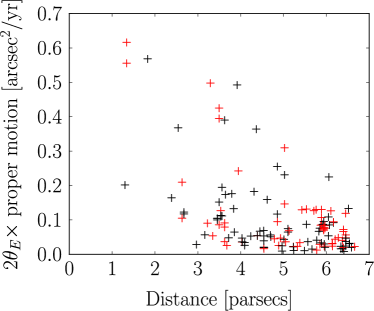
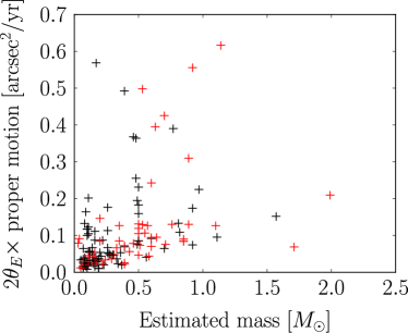
Figure 5: Sky area coming within one Einstein radius of each nearby star per year, plotted against distance (left), and against estimated stellar mass (right). Systems in red have been excluded from the discussion in Section 4.

If we restrict ourselves to masses $<0.5M_{\odot}$ and proper motions $>0\mbox{$.\!\!^{\prime\prime}$}5\rm\,/yr$, we are left with 85 stars. Assuming, as seen in our tests, that a galaxy within $10\,\theta_{E}$ is a candidate, we sum $20\,\mu\theta_{E}$ over these stars. The total available area is $\sim 70\,\rm arcsec^{2}$ per year.

The GalaxyCount program (Ellis & Bland-Hawthorn 2007) estimates $\simeq 1$ galaxy with magnitude $I\leq 25$ within a sky area of $70\,\rm arcsec^{2}$. This provides a rough estimate of the rate of observable weak microlensing events.

5 Observational Prospects

Observing the weak lensing of a faint galaxy by a nearby star would require a high resolution ($\approx 0\mbox{$.\!\!^{\prime\prime}$}05$) imager with high contrast capabilities. A $0.5M_{\odot}$ star at 5 pc has a brightness of $I\approx 6.5$mag while $I\approx 12$mag for a $0.1M_{\odot}$ star at the same distance. Thus a contrast in the range $\Delta I=12-18$mag must be achieved at a separation of about 0$.\!\!^{\prime\prime}$05 for typical events. This is quite a challenge for existing instruments. Fortunately, rapid progress can be expected in this field by instruments currently built for the imaging of planetary systems with 8m-10m telescopes and further significant progress will be possible with extremely large telescopes and high contrast imagers in space. They will provide very high contrast observations $\Delta m>20$mag and allow mass determinations of many nearby stars using weak microlensing of faint background galaxies as advocated in this Letter. Any background light that is not from the galaxy can still be considered part of the source as it will either be lensed or remain relatively constant throughout the duration of the complete observation program. An 8m class telescope with 30-50% efficiency collects about 50,000 photons/hr. Thus, a typical program might need between 20 and 100 hours to expect reasonable results.

With existing instruments it should already be possible to observe weak microlensing in favourable cases where the impact parameter is small and the optical resolution is higher than that considered here. Nearby ($d\approx 5$ pc) brown dwarfs with a mass of $\approx 0.05M_{\odot}$ ($\theta_{E}\approx 0\mbox{$.\!\!^{\prime\prime}$}01$) such as SCR 1845-6357 B (at 3.9 pc), DENIS 0255-4700 (5.0 pc), 2MASS 0415-0935 (5.7 pc), or GJ 570 D (5.9 pc), have $I\approx 17-20$ mag and $V\approx 22-25$ mag and they are not or not much brighter than the abundant backgound galaxies. Low mass stars and substellar objects are red or extremely red and imaging observations of blue star-forming galaxy at short wavelengths is favoured because the image contamination of the lensed galaxy by the PSF of the lensing object is strongly reduced. It seems that HST or an adaptive optics systems (e.g. with laser guide star) at a large telescope working at short wavelengths $<1\mu\rm m$ should be capable of achieving successful observations for certain weak microlensing events.

References

- Alcock et al. (1993) Alcock C., Akerlof C. W., Allsman R. A., et al. 1993, Nature, 365, 621
- An et al. (2002) An J. H., Albrow M. D., Beaulieu J.-P., et al. 2002, ApJ, 572, 521
- Aubourg et al. (1993) Aubourg E., Bareyre P., Bréhin S., et al. 1993, Nature, 365, 623
- Einstein (1936) Einstein A., 1936, Science, 84, 506
- Ellis & Bland-Hawthorn (2007) Ellis S. C., Bland-Hawthorn J., 2007, MNRAS, 377, 815
- Gould et al. (2006) Gould A., Udalski A., An D., et al. 2006, ApJ, 644, L37
- Gould et al. (2009) Gould A., Udalski A., Monard B., et al 2009, ApJ, 698, L147
- Henry (2009) Henry T. J., , 2009, RECONS, http://joy.chara.gsu.edu/RECONS/
- Lenzen et al. (2003) Lenzen R., Hartung M., Brandner W., et al. 2003, in M. Iye & A. F. M. Moorwood ed., Society of Photo-Optical Instrumentation Engineers (SPIE) Conference Series Vol. 4841 of Society of Photo-Optical Instrumentation Engineers (SPIE) Conference Series, NAOS-CONICA first on sky results in a variety of observing modes. pp 944–952
- Melchior et al. (2007) Melchior P., Meneghetti M., Bartelmann M., 2007, A&A, 463, 1215
- Paczyński (1996) Paczyński B., 1996, Acta Astronomica, 46, 291
- Refregier (2003) Refregier A., 2003, MNRAS, 338, 35
- Refsdal (1966) Refsdal S., 1966, MNRAS, 134, 315
- Rousset et al. (2003) Rousset G., Lacombe F., Puget P., et al. 2003, in P. L. Wizinowich & D. Bonaccini ed., Society of Photo-Optical Instrumentation Engineers (SPIE) Conference Series Vol. 4839 of Society of Photo-Optical Instrumentation Engineers (SPIE) Conference Series, NAOS, the first AO system of the VLT: on-sky performance. pp 140–149
- Saha (2003) Saha P., 2003, Principles of Data Analysis. Great Malvern, UK, Cappella Archive, 2003
- Udalski et al. (1993) Udalski A., Szymanski M., Kaluzny J., Kubiak M., Krzeminski W., Mateo M., Preston G. W., Paczynski B., 1993, Acta Astronomica, 43, 289