The Growth of Massive Galaxies Since $z=2$

Abstract

We study the growth of massive galaxies from $z=2$ to the present using data from the NEWFIRM Medium Band Survey (NMBS). The sample is selected at a constant number density of $n=2\times{}10^{-4}$ Mpc^-3, so that galaxies at different epochs can be compared in a meaningful way. We show that the stellar mass of galaxies at this number density has increased by a factor of $\approx{}2$ since $z=2$, following the relation $\log{}M_{n}(z)=11.45-0.15z$. In order to determine at what physical radii this mass growth occurred we construct very deep stacked rest-frame $R$ band images of galaxies with masses near $M_{n}(z)$, at redshifts $\langle{}z{}\rangle{}={}0.6$, 1.1, 1.6, and 2.0. These image stacks of typically 70-80 galaxies enable us to characterize the stellar distribution to surface brightness limits of $\sim{}28.5$ mag arcsec^-2. We find that massive galaxies gradually built up their outer regions over the past 10 Gyr. The mass within a radius of $r=5$ kpc is nearly constant with redshift whereas the mass at $5\,{\rm kpc}<r<75$ kpc has increased by a factor of $\sim{}4$ since $z=2$. Parameterizing the surface brightness profiles we find that the effective radius and Sersic $n$ parameter evolve as $r_{e}\propto(1+z)^{-1.3}$ and $n\propto(1+z)^{-1.0}$ respectively. The data demonstrate that massive galaxies have grown mostly inside-out, assembling their extended stellar halos around compact, dense cores with possibly exponential radial density distributions. Comparing the observed mass evolution to the average star formation rates of the galaxies we find that the growth is likely dominated by mergers, as in-situ star formation can only account for $\sim{}20$ % of the mass build-up from $z=2$ to $z=0$. A direct consequence of these results is that massive galaxies do not evolve in a self-similar way: their structural profiles change as a function of redshift, complicating analyses which (often implicitly) assume self-similarity. The main uncertainties in this study are possible redshift-dependent systematic errors in the total stellar masses and the conversion from light-weighted to mass-weighted radial profiles.

1. Introduction

Recent studies have found evidence that the structure of many massive galaxies has evolved rapidly over the past $\sim 10$ Gyr. Galaxies with stellar masses of $\sim 10^{11}$ ${\rm M}_{\odot}$ at $z=1.5-2.5$ are much more compact than galaxies of similar mass at $z=0$, particularly those with the lowest star formation rates (Daddi et al. 2005; Trujillo et al. 2006, 2007; Toft et al. 2007; Zirm et al. 2007; van Dokkum et al. 2008; Cimatti et al. 2008; van der Wel et al. 2008; Franx et al. 2008; Buitrago et al. 2008; Stockton et al. 2008; Damjanov et al. 2009; Williams et al. 2009). These findings are remarkable as massive galaxies at $z=0$ form a very homogeneous population, both in terms of their structure and their (old) stellar populations. As an example, the intrinsic scatter in the Fundamental Plane relation (Djorgovski & Davis 1987) is estimated to be $\lesssim 0.05$ dex for the most massive galaxies (e.g., Hyde & Bernardi 2009; Gargiulo et al. 2009), which seems difficult to reconcile with the dramatic changes implied by the measurements at $z\sim 2$.

Various interpretations of the high redshift data have been offered. Physical explanations for the apparent evolution from $z=2$ to $z=0$ include dramatic mass loss (Fan et al. 2008), (minor) mergers (Naab et al. 2007; Naab, Johansson, & Ostriker 2009; Bezanson et al. 2009), a fading merger-induced star burst (Hopkins et al. 2009c), and a combination of selection effects and mergers (van der Wel et al. 2009). All these models have some observational support, but it is not yet clear whether any single model is currently capable of simultaneously explaining the properties of galaxies at $z=2$ and at $z=0$.

The simplest explanation is that the data are interpreted incorrectly, due to errors in photometric redshifts, the conversion from light to stellar mass, the conversion from light-weighted to mass-weighted radii, or other effects. It is well known that absolute mass measurements of distant galaxies are very difficult, even with excellent data (see, e.g., Muzzin et al. 2009a,b for an extended discussion). Furthermore, sizes are typically determined from data that do not sample the profiles much beyond the effective radius $r_{e}$ (see, e.g., Hopkins et al. 2009a, Mancini et al. 2009), even though this is where most of the evolution may have taken place (e.g., Bezanson et al. 2009, Naab et al. 2009). Size measurements also require self-consistent procedures as a function of redshift, such as analyzing data in the same redshifted bandpass. It is easier to analyze imaging data in the rest-frame ultra-violet than in the rest-frame optical at high redshift (see, e.g., Trujillo et al. 2007, Mancini et al. 2009), but this requires large and unknown redshift-dependent corrections for color gradients. Despite these uncertainties, it is unlikely that the small sizes of high redshift galaxies can be entirely explained by errors, particularly given the consistency between different studies (see, e.g., van der Wel et al. 2008) and the first measurements of stellar kinematics (Cenarro & Trujillo 2009; van Dokkum, Kriek, & Franx 2009a; Cappellari et al. 2009). Nevertheless, subtle redshift-dependent biases are almost certainly present in the current data.

Ideally, we would measure the mass density profiles of galaxies well beyond $r_{e}$ for large and homogeneously selected samples as a function of redshift. In this paper, we take some steps in this direction by measuring the average surface brightness profiles of galaxies at $0<z<2$. We use new data from the NEWFIRM Medium Band Survey (NMBS), which provides accurate redshifts and deep photometry over a relatively wide area. Galaxies are selected at a constant number density rather than mass, which allows a more straightforward comparison of galaxies as a function of redshift than was possible in previous studies. The surface brightness profiles are measured from stacked images, which have a depth equivalent to $\sim 3000$ hrs of exposure time on a 4 m class telescope. This depth allows us to trace the surface brightness profiles to $\sim 28.5$ AB mag arcsec^-2, which is (just) sufficient to determine whether the outer envelopes of massive galaxies were already in place at early times.

As we show in this paper, a self-consistent description of the structural evolution of massive galaxies can be obtained from sufficiently deep and wide photometric surveys. Additional data and models such as those of Naab et al. (2009) and Hopkins et al. (2009c) are needed to better understand the physics driving this evolution. We assume $\Omega_{m}=0.3$, $\Omega_{\Lambda}=0.7$, and $H_{0}=70$ km s^-1 Mpc^-1. These parameters are slightly different from the WMAP five-year results (Dunkley et al. 2009) but allow for direct comparisons to most other recent studies of high redshift galaxies.

2. Sample Selection

2.1. The NEWFIRM Medium Band Survey

The sample is selected from the NMBS, a moderately wide, moderately deep near-infrared imaging survey (van Dokkum et al. 2009b). The survey uses the NEWFIRM camera on the Kitt Peak 4m telescope. The camera images a $28^{\prime}\times 28^{\prime}$ field with four arrays. The native pixel size is $0\farcs 4$; in the reduction the data are resampled to $0\farcs 3$ pixel^-1. The gaps between the arrays are relatively small, making the camera very effective for deep imaging of $0.25$ deg² fields. We developed a custom filter system for NEWFIRM, comprising five medium bandwidth filters in the wavelength range 1 $\mu$m – 1.7 $\mu$m. As shown in van Dokkum et al. (2009b) these filters pinpoint the Balmer and 4000 Å breaks of galaxies at $1.5<z<3$, providing accurate photometric redshifts and improved stellar population parameters. The survey targeted two $28^{\prime}\times 28^{\prime}$ fields: a subsection of the COSMOS field (Scoville et al. 2007), and a field containing part of the AEGIS strip (Davis et al. 2007). Coordinates and other information are given in van Dokkum et al. (2009b). Both fields have excellent supporting data, including extremely deep optical $ugriz$ data from the CFHT Legacy Survey and deep Spitzer IRAC and MIPS imaging (Barmby et al. 2006; Sanders et al. 2007). Reduced CFHT mosaics were kindly provided to us by the CARS team (Erben et al. 2009; Hildebrandt et al. 2009). The NMBS adds six filters: $J_{1}$, $J_{2}$, $J_{3}$, $H_{1}$, $H_{2}$, and $K$. Filter characteristics and AB zeropoints of the five medium band filters are given in van Dokkum et al. (2009b).

The NMBS is an NOAO Survey Program, with 45 nights allocated over three semesters (2008A, 2008B, 2009A). An additional 30 nights were allocated through a Yale-NOAO time trade. The data reduction, analysis, and properties of the catalogs are described in K. Whitaker et al., in preparation. In the present study we use a $K$-selected catalog based on data obtained in semesters 2008A and 2008B (version 3.1). The seeing in the combined images is $\approx 1\farcs 1$. All optical and near-IR images were convolved to the same point-spread function (PSF) before doing aperture photometry. The analysis in this paper is based on these PSF-matched images in order to limit bandpass-dependent effects. We note that not much could be gained by using the original images as the image quality varies only slightly between the different NEWFIRM bands. Following previous studies (Labbé et al. 2003; Quadri et al. 2007) photometry was performed in relatively small “color” apertures which optimize the S/N ratio. Total magnitudes in each band were determined from an aperture correction computed from the $K$ band data. The aperture correction is a combination of the ratio of the flux in SExtractor’s AUTO aperture (Bertin & Arnouts 1996) to the flux in the color aperture and a point-source based correction for flux outside of the AUTO aperture. We will return to this in § 2.2.

Photometric redshifts were determined with the EAZY code (Brammer, van Dokkum, & Coppi 2008), using the full $u-8\mu$m spectral energy distributions (SEDs) ($u-K$ for objects in the $\sim 50$ % of our AEGIS field that does not have Spitzer coverage). Publicly available redshifts in the COSMOS and AEGIS fields indicate that the redshift errors are very small at $\sigma_{z}/(1+z)<0.02$ (see Brammer et al. 2009). Although there are very few spectroscopic redshifts of optically-faint $K$-selected galaxies in these fields, we note that we found a similarly small scatter in a pilot program targeting galaxies from the Kriek et al. (2008) near-IR spectroscopic sample (see van Dokkum et al. 2009b).

Stellar masses and other stellar population parameters were determined with FAST (Kriek et al. 2009a), using the models of Maraston (2005), the Calzetti et al. (2000) reddening law, and exponentially declining star formation histories. Masses and star formation rates are based on a Kroupa (2001) initial mass function (IMF); following Brammer et al. (2008) rest-frame near-IR wavelengths are downweighted in the fit as their interpretation is uncertain (see, e.g., van der Wel et al. 2006). Rest-frame $U-V$ colors were measured using the best-fitting EAZY templates, as described in Brammer et al. (2009). More details are provided in Brammer et al. (2009) and, in particular, in K. Whitaker et al., in preperation.

2.2. A Number-Density Selected Sample

In many studies of galaxy formation and evolution changes in the galaxy population are traced through the evolution of scaling relations, such as the Fundamental Plane (see, e.g., van Dokkum & van der Marel 2007), the color-magnitude or color-mass relation (e.g., Holden et al. 2004), and relations between color, size, mass, and surface density (e.g., Trujillo et al. 2007; Franx et al. 2008). Other studies focus on evolution of the luminosity and mass functions, which trace changes in the number density of galaxies with particular properties (e.g., Fontana et al. 2006; Pérez-González et al. 2008; Marchesini et al. 2009). Finally, some studies combine information from scaling relations and luminosity functions. As an example, Bell et al. (2004), Faber et al. (2007) and others have inferred significant evolution in the red sequence at $0<z<1$ from the combination of accurate rest-frame colors and luminosity functions.

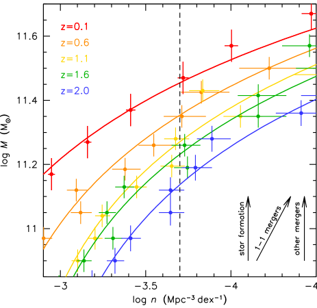
Figure 1.— Evolution of the stellar mass – number density relation at $0<z<2$, derived from Cole et al. (2001) and the NEWFIRM Medium Band Survey data. Arrows indicate the expected evolution for star formation, equal mass mergers, and mergers with mass ratios $<1$. For most astrophysical processes the most massive galaxies are expected to evolve along lines of constant number density, not constant mass. The dashed line shows the selection applied in this study: a constant number density of $n=2\times 10^{-4}$ Mpc^-3.

Here we follow a different and complementary approach, selecting galaxies not by their mass, luminosity, or color but by their number density. Figure 1 shows stellar mass as a function of number density (“rotated” mass functions) at five different redshifts. The $z=0.1$ mass function is taken from Cole et al. (2001) and converted to a Kroupa (2001) IMF. The points at higher redshift were all derived from the NMBS data, for $0.2<z<0.8$, $0.8<z<1.4$, $1.4<z<1.8$, and $1.8<z<2.2$. The datapoints were derived by determining the number density in bins of stellar mass. No further corrections were necessary as the completeness of the NMBS is $\approx 100$ % in this mass and redshift range (see Brammer et al. 2009, K. Whitaker et al., in preperation). The data shown in Fig. 1 are consistent with those in Marchesini et al. (2009), with smaller (Poisson) errors due to the much larger area of the NMBS. The lines are simple exponential fits to the points in the mass range $10.75<\log M<11.5$; mass functions from NMBS, including Schechter (1976) fits and a proper error analyis, will be presented in D. Marchesini et al., in preparation.

Arrows indicate schematically how galaxies may be expected to evolve. Star formation will, to first order, increase the stellar masses of galaxies and not change their number density. We note that this is strictly only true if the specific star formation rate (sSFR) is independent of mass, which is in fact not the case (see, e.g., Zheng et al. 2007; Damen et al. 2009). Mergers will change both the mass and the number density. However, because of the steepness of the mass function in this regime the effect is almost parallel to a line of constant number density, even for fairly major mergers. This is demonstrated for mergers with mass ratios $1:10$ – $1:2$ in Appendix A. We infer that selecting massive galaxies at a fixed number density enables us to trace the same population of galaxies through cosmic time, even as they form new stars and grow through mergers and accretion. Effectively, we assume that every massive galaxy today had at least one progenitor at $z=2$ which was also among the most massive galaxies at that redshift.

We choose a number density of $n=2\times 10^{-4}$ Mpc^-3 as the selection line in Fig. 1. The choice is a trade-off between the number of galaxies that enter the analysis at each redshift, the brightness of these galaxies, and the completeness of the sample at the highest redshifts. Figure 2 shows the mass evolution of galaxies at this number density, as given by the intersections of the exponential fits with the dashed line in Fig. 1. We verified that our results are not sensitive to the exact number density that is chosen here, by repeating key parts of the analysis for a number density of $1\times 10^{-4}$ Mpc^-3.

Figure 2.— The stellar mass of galaxies with a number density of $2\times 10^{-4}$ Mpc^-3, as a function of redshift. Errorbars are based on estimates of the amount of light that may be missed in our photometry; random errors are negligible. The observed mass evolution is very regular with small scatter. The solid line is a simple linear fit to the data, of the form $\log M_{n}=11.45-0.15z$. The dashed line has the form $\log M_{n}=11.48-0.67\log(1+z)$. The fits imply that galaxies with a stellar mass of $3\times 10^{11}$ ${\rm M}_{\odot}$ today assembled $\sim 50$ % of their mass at $0<z<2$. We note that unknown systematic uncertainties in the derived stellar masses have been ignored.

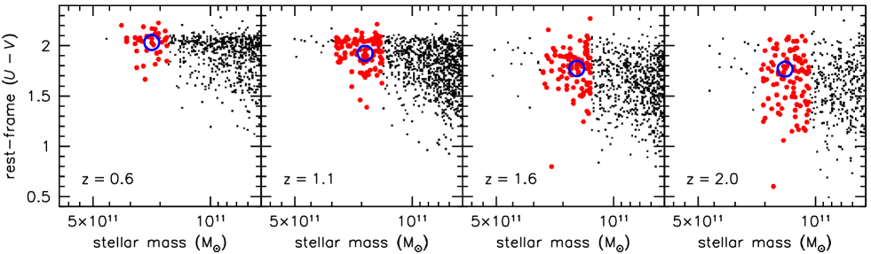
Figure 3.— Rest-frame $U-V$ color versus mass for galaxies in the NMBS. In each redshift bin galaxies were selected in a $\pm 0.15$ dex wide mass bin whose median mass is equal to $M_{n}$. Galaxies satisfying this criterion are highlighted in red. Out to $z\sim 1$ this selection includes mostly red galaxies. At higher redshifts an increasing fraction of the sample is blue. This is a real effect, and not due to photometric errors.

The solid line in Fig. 2 is a simple linear fit to the data of the form

$$\log M_{n}=11.45-0.15z.$$ (1)

The dashed line is an (equally good) fit of the form $\log M_{n}=11.48-0.67\log(1+z)$. Equation 1 implies mass growth by a factor of 2 since $z=2$ for galaxies with stellar masses of $3\times 10^{11}$ ${\rm M}_{\odot}$ today. The rms scatter in the residuals is very small at 0.017 dex, strongly suggesting that Poisson errors and field-to-field variations are small compared to other errors. A potential source of uncertainty is evolution in the fraction of light that is missed by our photometry. As discussed by, e.g., Wake et al. (2005) and Brown et al. (2007), the use of SExtractor’s MAG_AUTO aperture may lead to biases at faint magnitudes. We do not use MAG_AUTO itself but apply a correction based on the flux that falls outside the aperture (see Labbé et al. 2003). This correction is based on pointsources, which means it should be appropriate in our highest redshift bins where galaxies are small (see § 3.2). The correction may not be appropriate at $z=0.6$ and $z=1.1$, but at these redshifts the galaxies we select are extremely bright compared to the limits of our photometry, and the AUTO aperture is consequently large. From comparing the flux within the AUTO aperture to the integrated flux of the Sersic fits derived in § 3.4 we infer that the fraction of flux that is missed ranges from $\approx 5$ % at $z=2$ to $\approx 15$ % at $z=0.6$. The mass evolution from $z=2$ to $z=0.6$ may therefore be slightly underestimated, and we assign an error of $\pm 0.075$ dex to the mass in each redshift bin.

This estimate ignores other systematic errors in the masses, which are difficult to assess: uncertainties in stellar population synthesis codes, the IMF, the treatment of dust, star formation histories, and metallicities can easily introduce systematic errors of 0.2 – 0.3 dex (see, e.g., Drory, Bender, & Hopp 2004; van der Wel et al. 2006; Wuyts et al. 2009; Muzzin et al. 2009a; Marchesini et al. 2009). Many of these uncertainties are reduced as we are only concerned with the relative errors in the masses as a function of redshift; nevertheless, unknown systematics in the total masses are probably the largest source of error in our entire analysis.

2.3. Properties of the Sample

In practise, then, we select galaxies with masses near $\log M_{n}$ in the four redshift bins that we defined earlier, with $M_{n}$ given by Eq. 1. The width of each of the mass bins is fixed at $\pm 0.15$ dex and the exact bounds are chosen such that the median mass in the bin is equal to $M_{n}$. We have 39 galaxies in the $z=0.6$ bin, 108 at $z=1.1$, 96 at $z=1.6$, and 104 at $z=2.0$. The similarity of the number of objects in the three highest redshift bins is a reflection of our selection criterion and the fact that the volumes of these bins are roughly equal (see Table 1).

Figure 3 shows where the selected galaxies fall in the color-mass plane in each redshift bin. In the lowest redshift bins galaxies of this number density are nearly always red, but the range of rest-frame colors increases as we go to higher redshift. This increase is real and not due to photometric errors, as the S/N ratio of the NMBS photometry is high in this mass and redshift range. Brammer et al. (2009) use these same data to demonstrate that the range in colors out to $z=2$ reflects real stellar population differences between the galaxies. Note that we do not make any cuts on color, star formation rate, or other properties as we are interested in the full set of progenitors of today’s massive galaxies.

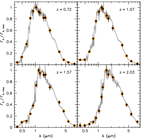
Figure 4.— Spectral energy distributions of typical galaxies in the four redshift bins, illustrating the high quality of our photometric data. The locations of these galaxies in the color-mass plane are indicated by blue circles in Fig. 3. Data points are $u$, $g$, $r$, $i$, $z$ from the Deep CFHT Legacy Survey, $J_{1}$, $J_{2}$, $J_{3}$, $H_{1}$, $H_{2}$, and $K$ from the NMBS, and IRAC channel 1–4. The grey line shows the best-fitting EAZY template (Brammer et al. 2008). Note that the medium band filters are critical for determining the redshifts and SED shapes for galaxies in this mass and redshift range.

The data quality is illustrated in Fig. 4, which shows the observed SEDs of four galaxies whose redshifts, rest-frame $U-V$ colors and stellar masses are close to the medians in each redshift bin. The locations of these galaxies in the color – mass plane are indicated in Fig. 3 with blue circles. The SEDs illustrate the important role of the medium-band near-IR filters in the analysis; typical massive galaxies at high redshift are faint in the rest-frame ultra-violet (see also, e.g., van Dokkum et al. 2006), and critical features for determining redshifts and stellar population parameters are shifted beyond $\sim 1\,\mu$m. This point was also made by Ilbert et al. (2009), who show that even with 30 photometric bands (including medium-band optical data from Subaru, but not including medium near-IR bands) photometric redshifts in the range $1.5<z<3$ are highly uncertain.

In the present study we are not concerned with (subtle) changes in the stellar populations of the galaxies as a function of redshift. Stacked rest-frame SEDs of NMBS galaxies with different redshifts, masses, and rest-frame colors will be presented in K. Whitaker et al., in preperation. Brammer et al. (2009) discuss the origin of the scatter in the color-magnitude plane, demonstrating that dusty star-forming galaxies make up most of the “green valley” objects at $0<z<2$.

TABLE 1
Properties of Stacked Images
$z=0$ $\langle z\rangle=0.6$ $\langle z\rangle=1.1$ $\langle z\rangle=1.6$ $\langle z\rangle=2.0$ Source OBEY NMBS NMBS NMBS NMBS $z$ range — $0.2-0.8$ $0.8-1.4$ $1.4-1.8$ $1.8-2.2$ $V^{(1)}$ — 0.89 2.28 1.93 2.06 $\log M_{n}^{(2)}$ 11.45 11.36 11.28 11.21 11.15 $N^{(3)}$ 14 39 108 96 104 $N_{\rm clean}^{(4)}$ 14 32 87 73 79 $r_{e}^{(5)}$ $12.4^{1.6}_{-1.3}$ $8.0^{+1.2}_{-0.5}$ $5.3^{+0.3}_{-0.1}$ $4.1^{+0.2}_{-0.3}$ $3.0^{+0.4}_{-0.2}$ $n^{(6)}$ $5.9^{+0.7}_{-0.6}$ $4.0^{+0.4}_{-0.4}$ $2.9^{+0.2}_{-0.2}$ $2.5^{+0.2}_{-0.2}$ $2.1^{+0.5}_{-0.4}$ $\langle{\rm SFR}\rangle^{(7)}$ — $0.8^{+0.3}_{-0.3}$ $2.5^{+1.1}_{-1.2}$ $19^{+9}_{-9}$ $55^{+14}_{-13}$

(1) Volume in units of $10^{6}$ Mpc³.
(2) Median of mass bin, in units of ${\rm M}_{\odot}$. The stacks are normalized such that $\int_{0}^{75\,{\rm kpc}}2\pi r\Sigma(r)dr=M_{n}$, with $\Sigma(r)$ the best-fitting Sersic profile.
(3) Number of galaxies in mass bins of width $0.3$ dex. Note that the densities plotted in Fig. 1 are in units of Mpc^-3 dex^-1.
(4) Number of galaxies remaining after visual inspection.
arcsec².
(5) Best-fitting effective radius in kpc.
(6) Best-fitting Sersic (1968) $n$ parameter.
(7) Mean star formation rate in units of ${\rm M}_{\odot}$ yr^-1.

3. Analysis

3.1. Creating Stacked Images

Most studies of the size evolution of distant galaxies measure effective (i.e., half-light) radii for individual galaxies and then analyze the evolution of the mean (or median) size, typically at fixed stellar mass (e.g., Trujillo et al. 2007; van Dokkum et al. 2008; van der Wel et al. 2008, and many others). Here we follow a different approach, which emphasizes the strengths of our dataset: uniform, deep imaging of a large, objectively defined sample. Instead of measuring sizes and then taking the average we first create averaged images and then measure sizes. In Appendix B we show that the average circularized effective radius and the Sersic (1968) $n$ parameter can both be recovered from stacked images of large numbers of galaxies. The key advantage of this approach is that it enables the detection of the faint outer regions of galaxies, which are now thought to evolve much more strongly than the central regions (e.g., Naab et al. 2007, 2009; Hopkins et al. 2009c; Bezanson et al. 2009). Rather than parameterizing structural evolution with changes in $r_{e}$ only we can characterize the evolution of the full surface density profiles. An important practical advantage is that we do not need data of very high spatial resolution. At $\approx 1\farcs 1$ the resolution of the NEWFIRM data is mediocre even for ground-based data – but as we show later this does not prohibit us from tracking the dramatic changes in galaxy profiles at radii of 5 kpc – 50 kpc.

The stacked images were created by adding normalized, masked images of the individual galaxies in each redshift bin. Image “stamps” of individual objects were cut from the NMBS images. The stamps are $80\times 80$ pixels, corresponding to $24\arcsec\times 24\arcsec$. Images in individual NEWFIRM bands were summed to increase the S/N ratio. The bands were selected so that the images are approximately in the same rest-frame band. Galaxies in the $z=0.6$ redshift bin were taken from a summed $J_{1}$ + $J_{2}$ image, galaxies at $z=1.1$ from $J_{3}$ + $H_{1}$, galaxies at $z=1.6$ from $H_{1}$ + $H_{2}$, and galaxies at $z=2.0$ from $H_{2}$ + $K$. The corresponding rest-frame wavelengths are close to the rest-frame $R$ band: $\lambda_{0}=0.70\,\mu$m, $0.68\,\mu$m, $0.63\,\mu$m, and $0.65\,\mu$m for $z=0.6$, $z=1.1$, $z=1.6$, and $z=2.0$ respectively. The galaxies were shifted so that they are centered as closely as possible to the center of the central pixel, using subpixel shifts with a third-order polynomial interpolation.

A mask was created for each object, flagging pixels that are potentially affected by neighboring galaxies. This mask image was constructed in the following way. First, SExtractor was run with a very low detection threshold on a combined $J_{3}$ + $H_{1}$ + $H_{2}$ + $K$ image. A “red” mask was created by flagging all positive pixels in the segmentation map except those belonging to the central object. This mask identifies flux from red objects and bright blue objects but does not include flux below the detection threshold from the numerous faint, blue objects that are present in any $24\arcsec\times 24\arcsec$ image of the sky. These objects were identified in a combined $g+r+i$ image, constructed from the PSF-matched CFHT Legacy Survey images. These data are extremely deep, reaching $\approx 29$ mag (AB) at $5\sigma$ in a $1\farcs 2$ aperture. With our low detection threshold approximately half of all pixels are flagged in the blue mask. The final mask is created by combining the blue and the red mask. The red mask is not redundant, as a non-negligible number of objects detected in the NEWFIRM images are absent in the combined $g+r+i$ image.

The masked images were visually inspected to identify blended or unmasked objects, star spikes, and other obvious problems. This step is necessary as objects that were flagged as (de-)blended by SExtractor were not removed from the initial catalogs: given the large size and large apparent brightness of the galaxies in the lowest redshift bins a blind rejection would have introduced redshift-dependent selection effects. Approximately 25 % of objects were removed at this stage. We verified that the final profiles are not very dependent on this step; the only individual galaxies which have a significant impact on the stacks are the few cases where there are obviously two unmasked objects in the image. Next, the images were normalized using the flux in a $10\times 10$ pixel ($3\arcsec\times 3\arcsec$) square aperture. The stacked images are nearly identical when the catalog flux is used instead (in either a fixed aperture or the aperture-corrected flux). For completeness, the final pre-stack images of all galaxies are shown in Appendix C.

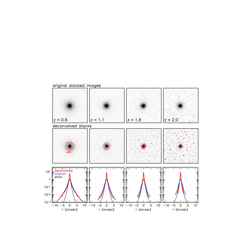
Figure 5.— Top panels: stacked images of galaxies with constant number density in four redshift bins. Each image is $24\arcsec\times 24\arcsec$. The images reach surface brightness levels of $\sim 28.5$ AB mag arcsec^-2, and correspond to $\sim 3000$ hrs of total exposure time on a 4m class telescope. Middle panels: Deconvolved stacks, highlighting the fact that the radial extent of the low surface brightness emission decreases with redshift. Broken (solid) contours show the radii where the flux is 5 % (0.5 %) of the peak flux. The 5 % contour is similar at all redshifts, but the 0.5 % contour evolves rapidly. Bottom panels: Radial surface brightness profiles, normalized to the peak flux in the original stacks. Observed profiles are shown in blue, deconvolved profiles in red. The black curve is for stacked images of stars. The galaxies are resolved at all redshifts, and are progressively smaller at higher redshifts.

Stacked images were created by summing the individual images. The masks were also summed, effectively creating a weight map. Average, exposure-corrected stacked images were created for each redshift bin by dividing the raw stacks by the weight maps. The background value at large radii is slightly negative: the object masks used in the reduction are not as conservative as the masks used here, leading to a slight overestimate of the background in the reduction. Expressed in AB surface brightness the background error is $\approx 28$ mag arcsec^-2. We correct for the oversubtracted background in a straightforward way, by defining the total flux of a galaxy as the flux within a 75 kpc radius. This radius corresponds to $\approx 7r_{e}$ for bright elliptical galaxies at $z=0$, and many tens of effective radii for high redshift galaxies. In practise, the average value of pixels with $r>75$ kpc is subtracted from each of the stacks. This procedure is very robust; bootstrapping the stacks (see § 3.3) shows that the uncertainty in the background correction is only a few percent. Finally, the images are divided by the total flux in the image. The final stacks therefore have a total flux of 1 within a 75 kpc radius aperture and a mean flux of zero outside of this aperture.

3.2. Surface Brightness Profiles

The observed stacks are shown in the top panels of Fig. 5. There are no obvious residuals in the background, thanks to the aggressive masking. The images are very deep: the surface brightness profiles can be traced to levels of $\sim 28.5$ AB mag arcsec^-2 in the observed frame. For the $z=0.6$ stack these levels are reached at radii of $\sim 70$ kpc ($\sim 10\arcsec$); as we show later this corresponds to $\sim 10$ effective radii. The depth is slightly larger for the $z=0.6$ and $z=1.1$ stacks than for the higher redshift stacks: the $J_{x}$ band images are deeper than the $H_{x}$ and $K$ band data when expressed in AB magnitudes, and the ellipse fitting routine averages over more pixels for the low redshift galaxies as they are more extended (as we show later).

The stellar PSF is fairly broad in this study, with a full width at half maximum (FWHM) of $\approx 1\farcs 1$, and we first investigate whether the observed stacks are resolved at this resolution. Radial surface brightness profiles of the stacked images are shown in blue in the bottom panels of Fig. 5. Black curves show the profiles of stacked images of stars, derived from the same data. The stars were identified based on their colors (see K. Whitaker et al., in preparation) in a narrow magnitude range similar to the galaxies in the sample. They were shifted, masked, visually inspected, averaged, and normalized in the same way as the galaxy images. The galaxy profiles and the stellar profiles were normalized to a peak flux of 1. The blue curves are broader than the black curves at all redshifts, demonstrating that the galaxies are resolved.

To investigate the behavior of the galaxy profiles with redshift the stacks were deconvolved using carefully constructed PSFs. The PSFs were created by averaging images of bright unsaturated stars, masking companion objects. The COSMOS and AEGIS fields have slightly different PSFs; for each stack a separate PSF was constructed using the appropriate filters and appropriately weighting the PSFs of the two fields. As a test, we repeated the analysis using the stacked stellar images described above. Differences were small and not systematic; the differences in the measured effective radii were $<10$ % at all redshifts. The deconvolution was done with a combination of the Lucy-Richardson algorithm (Lucy 1974) and $\sigma$-CLEAN (Högbom 1974; Keel 1991), ensuring flux conservation. Lucy works well for extended low surface brightness emission but does not optimally recover the flux in the central pixels (see, e.g., Griffiths et al. 1994), whereas CLEAN quickly converges in the central regions but leads to strong amplification of noise in areas of low surface brightness. In practice, we applied a smoothly varying weight function to combine the CLEAN and Lucy reconstructions, giving a weight of 1 to CLEAN in the central pixels and a weight of 1 to Lucy at radii $>3$ pixels. In the transition region the form of the weight function was determined by the requirement to conserve total flux. We note that we use the deconvolved images for illustrative purposes only, as we later quantify the evolution by fitting Sersic (1968) profiles to the original, PSF-convolved images. The deconvolved images are shown below the original stacks in Fig. 5. Profiles derived from these images are shown in red in the bottom panels of Fig. 5.

It is immediately obvious from the deconvolved images and the radial profiles that the galaxies are smaller at higher redshift. Furthermore, the central parts of the galaxies are fairly similar: at all redshifts there is a bright core but only at lower redshifts this core is surrounded by extended emission. This is a key result of the paper and it is quantified in the sections below. Here it is illustrated by the red contours in Fig. 5. The inner (dotted) contour shows the radius at which the surface brightness is 5 % of the peak value. This radius is very similar at all redshifts. The outer (solid) contour shows the radius where the surface brightness if $0.5$ % of the peak. This radius is much larger at low redshift than at high redshift. Together, the two contours demonstrate that the shape of the profile changes with redshift, with the core of present-day massive galaxies mostly in place at $z=2$ but the outer parts building up gradually over time.

3.3. Surface Density Profiles

When color gradients are ignored, the deconvolved radial profiles can be interpreted as stellar mass surface density profiles. The median mass of the galaxies in each of the stacks is determined by our constant number density selection, and the calibration of the profiles follows from the requirement that

$$\int_{0}^{75}2\pi r\Sigma(r)dr=M_{n},$$ (2)

with $r$ in kpc, $\Sigma(r)$ the radial surface density profile in units of ${\rm M}_{\odot}$ kpc^-2, and $M_{n}$ given by Eq. 1. It is implicitly assumed that the total stellar mass in our catalog equals the mass within a 150 kpc diameter aperture (see § 2.2). Figure 6 shows the radial surface density profiles as a function of redshift. Errorbars are 68 % confidence intervals determined from bootstrapping: 500 realizations were created of each of the stacks, and we followed the same analysis steps on these as for the actual stacks. This method is more robust than a formal analysis of the noise, as it includes errors due to improper masking of particular objects, uncertainties in the background subtraction, and uncertainties due to real variation in the properties of galaxies that enter the stack. We note here that color gradients are almost certainly important (see § 4.3), but that it is at present difficult to correct for them.

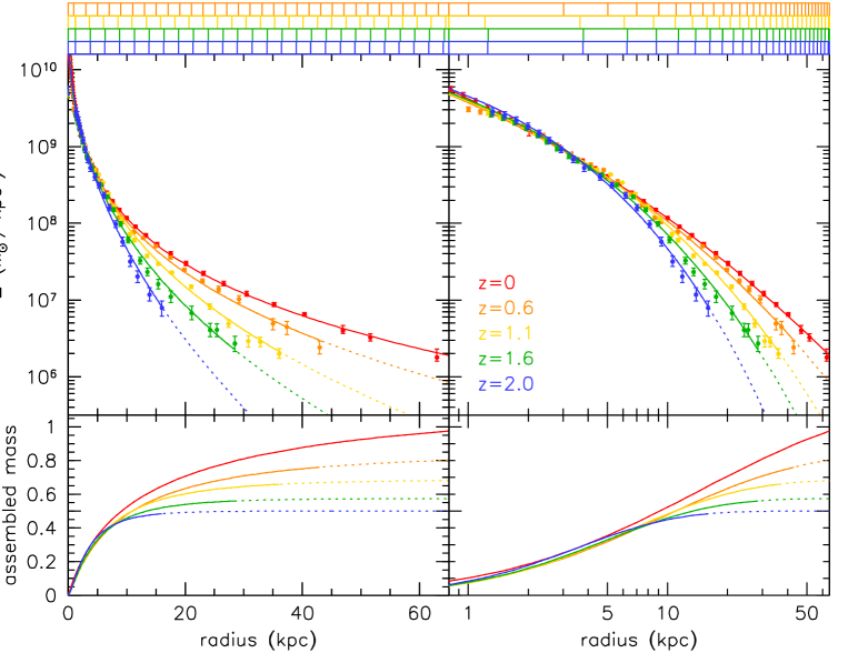
Figure 6.— Top panels: Average radial surface density profiles of galaxies with a number density of $2\times 10^{-4}\,$Mpc^-3 as a function of redshift. The data points were measured from the deconvolved stacked images. Errorbars are 68 % confidence limits derived from bootstrapping the stacks. The same data are shown versus radius (left panel) and log radius (right panel). Small boxes above the panels indicate the pixel size of $0\farcs 3$. There is a clear trend with redshift: at small radii the profiles overlap, but at large radii the profiles get progressively steeper with redshift. Lines show the best-fitting Sersic profiles, determined from fitting PSF-convolved models to the original (not deconvolved) stacked images. Bottom panels: Cumulative mass as a function of radius, as implied by the best-fitting Sersic profiles. The vertical axis is in units of the total mass at $z=0$ within a 150 kpc diameter aperture. Note that the normalization of the profiles is not a free parameter but follows from the requirement that the total mass within this aperture is equal to $M_{n}(z)$ (Eq. 1). The mass growth of galaxies of this number density is dominated by the build-up of the outer envelope, at radii $\gtrsim 5$ kpc.

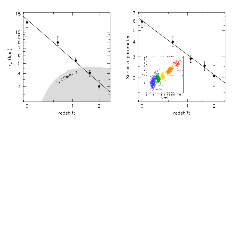
Figure 7.— Evolution of the effective radius $r_{e}$ (left panel) and the Sersic parameter $n$ (right panel) for galaxies with a number density of $2\times 10^{-4}$ Mpc^-3. Errors are 68 % confidence intervals determined from repeating the analysis on bootstrapped realizations of the stacked images. Individual measurements from these realizations are shown in the inset. The grey area indicates where the effective diameter is smaller than the FWHM of the PSF. Galaxies have smaller effective radii at higher redshift and profiles that are closer to exponential.

The profile for $z=0$ was determined from the Observations of Bright Ellipticals at Yale (OBEY) survey (Tal et al. 2009). This survey obtained surface photometry out to very large radii for a volume-limited sample of luminous elliptical galaxies. A stacked image was created and analyzed in the same way as was done for the NMBS galaxies; details are given in Appendix D. As discussed in the Appendix, the OBEY $z=0$ stacked image should be directly comparable to the NMBS stacks at higher redshift. Also, its surface density profile was normalized using Eq. 2 and is therefore on the exact same system as the NMBS galaxies.

The surface density profiles display a striking evolution with redshift. At $z=0$, the profile shows the dense center and extended outer envelope familiar from numerous studies of elliptical galaxies. At higher redshift, the profiles in the central regions remain virtually unchanged but they become progressively steeper at large radii. The extended outer envelope of elliptical galaxies appears to have been built up gradually since $z=2$ around a compact core that was formed at higher redshift. Our data obviously lack the resolution to properly determine the shape of the profiles in the central 5 kpc; nevertheless, flux conservation implies that they cannot be significantly steeper or flatter than what is shown in Fig. 6. More to the point, the data do have sufficient depth and resolution to track the emergence of the outer envelope at radii $>5$ kpc, although even deeper data would be valuable at $z=2$. A possible concern is that subtle redshift-dependent effects drive (part of) the evolution at large radii. We tested this explicitly in Appendix B, where we redshift the $z=0$ and $z=0.6$ data to $z=2$ and show that the derived evolution is robust.

3.4. Sersic Fits

The profiles are parameterized with standard Sersic (1968) fits, of the form

$$\Sigma_{b}(r)=\Sigma_{e}10^{-b_{n}[(r/r_{e})^{1/n}-1]},$$ (3)

where $\Sigma(r)$ is the surface brightness at radius $r$, $b_{n}$ is a constant that depends on $n$, $n$ is the “Sersic index”, and $r_{e}$ is the radius containing 50 % of the light. These fits are performed on the original stacked images, by fitting models convolved with the PSF. This approach has the advantage that it uses a convolution rather than a deconvolution. The fits were done with GALFIT (Peng et al. 2002). They converged quickly, and the parameters do not depend on the choice of fitting region, initial guesses for the parameters, and whether the sky is left as a free parameter. The fits were normalized using Eq. 2 and therefore give the correct masses within a 150 kpc diameter aperture.

The Sersic fits are shown by the lines in the top panels of Fig. 6. The lines follow the datapoints quite well, indicating that the deconvolutions did not produce large systematic errors in the profiles. The bottom panels of Fig. 6 show the cumulative radial mass profiles as implied by the Sersic fits. The vertical axis is in units of the total mass within a 150 kpc diameter aperture at $z=0$, i.e., $2.8\times 10^{11}$ ${\rm M}_{\odot}$. The mass contained within $\sim 5$ kpc is remarkably similar at all redshifts, and essentially all the mass growth is at large radii.

The evolution in the shape of the radial surface density profiles is parameterized by evolution in the effective radius and in the Sersic parameter $n$. The profiles are both more concentrated and closer to exponential at redshifts $z>1.5$. This is demonstrated in Fig. 7, which shows the evolution in $r_{e}$ and $n$. Errorbars are 68 % confidence limits determined from bootstrapping the stacks. We note that our fitting procedure, and particularly the definition of total mass (Eq. 2), leads to subtle and redshift-dependent correlations of the errors. The inset in Fig. 7 shows individual measurements of $r_{e}$ and $n$ from the bootstrapped stacks. Correlations exist but they are not sufficiently large to influence our results. The lines are fits to the data of the form

$$r_{e}=13.2\times(1+z)^{-1.27}$$ (4)

and

$$n=6.0\times(1+z)^{-0.95}.$$ (5)

The formal errors in these relations are small and the scatter in the residuals is small: 0.029 in $\log r_{e}$, and $0.015$ in $\log n$. Together with Eqs. 1 and Eq. 2 these expressions provide a complete description of the evolution of the stellar mass in galaxies with a number density of $2\times 10^{-4}$ Mpc^-3, as a function of redshift and radius.

The evolution in the effective radius is a factor of $\sim 4$, whereas the mass evolves by a factor of $\sim 2$. The evolution in the familiar radius-mass diagram (see, e.g., Trujillo et al. 2007) is shown in Fig. 8. The solid line is a fit to the OBEY and NMBS data; the slope implies that $r_{e}\propto M^{2.04}$. In addition to the OBEY data we show the mass-size relation for massive early-type galaxies from Guo et al. (2009) (SDSS) and the average of four Virgo ellipticals from Kormendy et al. (2009) (see Appendix D). The $z=0$ data are in good agreement with each other and also with an extrapolation of the NMBS data to lower redshift. Open circles show the median sizes of galaxies in the GOODS CDF-South field, as determined by the FIREWORKS survey (Wuyts et al. 2008; Franx et al. 2008). The CDF-South is a much smaller field (by a factor of $>10$), but the imaging data is of very high quality (see Franx et al. 2008). The CDF-South data are in excellent agreement with our results, although we note that the uncertainties are large as there are only 10–15 galaxies in each of the bins. Finally, we note that the sizes of the $z=2$ galaxies are a factor of $\sim 3$ larger than the median of nine quiescent galaxies at $z=2.3$ (van Dokkum et al. 2008). The reason is that we include all galaxies in the analysis, not just quiescent ones, and as is well known star forming galaxies are significantly larger than quiescent galaxies (e.g., Toft et al. 2007; Zirm et al. 2007; Franx et al. 2008, Kriek et al. 2009b).

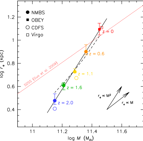
Figure 8.— Evolution in the radius-mass plane. Our data are consistent with measurements for individual galaxies of the same masses and redshifts in the FIREWORKS CDF-South survey of Wuyts et al. (2008) and Franx et al. (2008) (open circles). Our $z=0$ point from the OBEY survey (Tal et al. 2009) is consistent with data from Virgo ellipticals by Kormendy et al. (2009) and a recent determination of the mass-size relation in the SDSS (Guo et al. 2009). The evolution in effective radius is stronger than in mass: the solid line is a fit of the form $r_{e}\propto M^{2.04}$. The dashed line is the expected evolution of the effective radius for inside-out growth, calculated using Eq. 7 and the measured value of the Sersic index $n$ at each redshift.

4. Discussion

4.1. Inside-Out Growth

As demonstrated in § 2.2 and § 3 galaxies with a space density of $2\times 10^{-4}$ ${\rm M}_{\odot}$ Mpc^-3 increased their mass by a factor of $\approx 2$ since $z=2$, apparently mostly by adding stars at large radii. The radial dependence of the evolution can be assessed by integrating the deprojected density profiles of the galaxies. Following Ciotti (1991) the surface density profiles were converted to mass density profiles using an Abel transformation. The mass in the central regions can then be determined by integrating these mass density profiles from zero to a fixed physical radius (see Bezanson et al. 2009). Bezanson et al. (2009) used a radius of 1 kpc, which corresponds to the typical effective radii of quiescent galaxies at $z\sim 2.3$. In our data 1 kpc corresponds to a small fraction of a single pixel, and we use a fixed radius of 5 kpc instead.

The evolution of the mass within 5 kpc is shown in Fig. 9 by the red datapoints. Errors were determined from 500 bootstrapped realizations of the stacks. Also shown are the evolution of the total mass and the evolution of the mass outside a fixed radius of 5 kpc. Note that each of the stacks is normalized to give exactly the total mass of Eq. 1; the total mass has therefore no errorbar in Fig. 9 and the errorbars on the red and blue data points are directly coupled. The mass within a fixed aperture of 5 kpc is approximately constant with redshift at $\approx 10^{10.9}$ ${\rm M}_{\odot}$, whereas the mass at $r>5$ kpc has increased by a factor of $\sim 4$ since $z=2$.

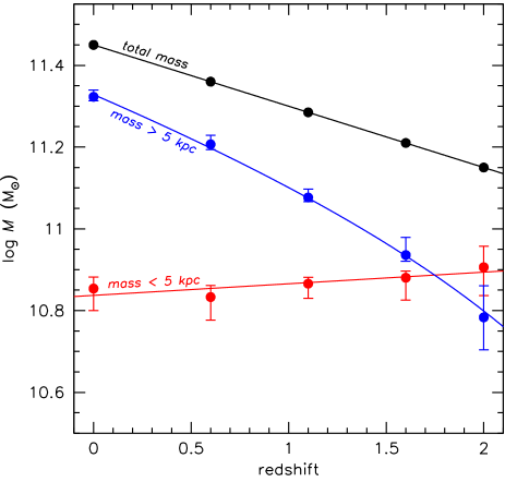
Figure 9.— Comparison of the mass contained within a fixed radius of 5 kpc (red curve) to the mass at larger radii (blue curve), as a function of redshift. Errorbars are 95 % confidence limits derived from bootstrapping. The total mass is shown in black. Galaxies with number density $n=2\times 10^{-4}$ Mpc^-3 have a nearly constant mass in the central regions. The factor of $\approx 2$ increase in total mass since $z=2$ is driven by the addition of stars at radii $>5$ kpc.

It is interesting to consider the expected evolution of galaxies in the radius-mass diagram (Fig. 8) in this context. As discussed in, e.g., Bezanson et al. (2009) and Naab et al. (2009), the change in radius for a given change in mass provides important information on the physical mechanism for growth. Major mergers are expected to result in a roughly linear relation, $d\log(r_{e})/d\log(M)\sim 1$, whereas minor mergers could give values closer to 2. There is, however, also a simple geometrical effect resulting from the shape of the Sersic profile and the definition of the effective radius. If mass is added to a galaxy the effective radius has to change so that it still encompasses 50 % of the total mass. If the added mass is small and at $r\gg r_{e}$ the form of the density profile at $r\approx r_{e}$ will not change appreciably, even in projection. The change in effective radius for a given change in mass is then simply the inverse of the derivative of the enclosed mass profile,

$$\frac{d\log(r)}{d\log(M)}=\left\{\frac{d\log\left[\int_{0}^{r}2\pi r\Sigma(r)dr\right]}{d\log r}\right\}^{-1},$$ (6)

evaluated at $r=r_{e}$. Numerically solving Eq. 6 gives a simple relation between the Sersic index $n$ and the change in effective radius for a given change in mass:

$$\frac{d\log(r_{e})}{d\log(M)}\approx 3.56\log(n+3.09)-1.22.$$ (7)

This relation is accurate to $0.01$ dex for $1\leq n\leq 6$.

Equation 7 implies that the effective radius increases approximately linearly with mass if the projected density follows an exponential profile, but as $r_{e}\propto M^{1.8}$ for a de Veaucouleurs profile with $n=4$. This in turn implies that strong evolution in the measured projected effective radius can be expected in all inside-out growth scenarios irrespective of the physical mechanism that is responsible for that growth, unless the projected density profiles are close to exponential. The predicted change in $r_{e}$ as a function of mass based on Eq. 7 is indicated with a dashed line in Fig. 8, calculated using the measured values of $n$ at each redshift. As might have been expected, the line closely follows the observed data points.

4.2. Star Formation versus Mergers

Several mechanisms have been proposed to explain the growth of massive galaxies. The simplest is star formation, which can be expected to play an important role at higher redshifts as a large fraction of massive galaxies at $z\sim 2$ have high star formation rates (e.g., van Dokkum et al. 2004; Papovich et al. 2006). Franx et al. (2008) expressed the evolution in terms of surface density, and found that many galaxies with the (high) surface densities of $z=0$ early-type galaxies were forming stars at $z=1-2$. However, the old stellar ages of the most massive early-type galaxies (e.g., Thomas et al. 2005; van Dokkum & van der Marel 2007) and the existence of apparently “red and dead” galaxies with small sizes at $z=1.5-2.5$ (e.g., Cimatti et al. 2008; van Dokkum et al. 2008) suggest that at least some of the growth is due to (“dry”) mergers. Growth by mergers is expected in $\Lambda$CDM galaxy formation models (e.g., De Lucia et al. 2006), and could be effective in growing the outer envelope of elliptical galaxies (Naab et al. 2007, 2009; Bezanson et al. 2009).

We can assess the contributions of star formation and mergers to the assembly of the outer parts of massive galaxies as we have independent measurements of the total mass growth and the growth due to star formation. The solid line in Figure 10 shows the measured net mass growth (Eq. 1) expressed in ${\rm M}_{\odot}$ yr^-1. Galaxies with a number density of $2\times 10^{-4}$ Mpc^-3 have added mass to their outer regions at a net rate that declined from $\approx 30$ ${\rm M}_{\odot}$ yr^-1 at $z=2$ to $\approx 10$ ${\rm M}_{\odot}$ yr^-1 today.

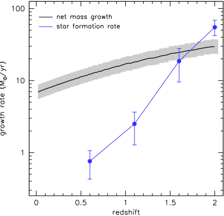
Figure 10.— Growth rate of the galaxies as a function of redshift, in ${\rm M}_{\odot}$ yr^-1. The net growth rate, derived from the mass evolution at fixed number density, is indicated with the black line. The shaded region indicates the $1\sigma$ uncertainty (see § 2.2). Blue points with errorbars show the average star formation rate of the galaxies in each of the stacks, as derived from fits of stellar population synthesis models to their SEDs. Star formation can account for most or all of the observed growth at $z=1.5-2$, but not for the continued growth at lower redshifts.

The net mass growth is determined by a combination of mass growth due to star formation, mass growth due to mergers, and mass loss due to winds:

$$\dot{M}_{\rm net}=\dot{M}_{\rm SFR}+\dot{M}_{\rm mergers}-\dot{M}_{\rm winds}.$$ (8)

The blue points in Fig. 10 show the mean star formation rate $\dot{M}_{\rm SFR}$ of the galaxies that enter each of the stacks. The star formation rates were determined from fits of stellar population synthesis models to the observed SEDs of the individual galaxies (see § 2.1). The errorbars were determined from boostrapping and do not include systematic uncertainties. As is well known, uncertainties in the star formation histories, dust content and distribution, the IMF, and other effects can easily introduce systematic errors of a factor of $\sim 2$ in the star formation rates, particularly at high redshift (see, e.g., Reddy et al. 2008; Wuyts et al. 2009; Muzzin et al. 2009a). The average star formation rate is similar to the net growth rate at $z=1.5-2$ but significantly smaller at later times. We infer that the growth of the outer parts of massive galaxies is not due to a single process but due to a combination of star formation and mergers. Star formation is only important at the highest redshifts, and the growth at $z=0-1.5$ is dominated by mergers.

It is interesting to consider whether the decline in the star formation rate at $z<1.5$ is directly related to the structural evolution of the galaxies. The specific star formation rate of galaxies correlates well with the average surface density of galaxies within the effective radius, $\langle\Sigma\rangle=0.5M_{\rm star}/(\pi r_{e}^{2})$, and there is good evidence for a surface density threshold above which star formation is very inefficient (Kauffmann et al. 2003b, 2006). Recently Franx et al. (2008) have shown that this correlation exists all the way to $z\sim 3$, and that the threshold evolves with redshift. The average surface density of galaxies in our study follows directly from the masses and radii; since $r_{e}\propto(1+z)^{-1.3}$ and $M\propto(1+z)^{-0.7}$, we find that $\Sigma\propto(1+z)^{2}$. Interestingly, the surface densities of our galaxies are close to the threshold surface density of Franx et al. (2008) and Kauffmann et al. (2003b) above which little or no star formation takes place. We note that these studies focus on galaxies with lower, more typical masses than the extreme objects considered here. Franx et al. (2008) noted that the specific star formation rate may be better correlated with (inferred) velocity dispersion than with surface density. We later estimate velocity dispersions for our galaxies, and these do indeed imply little star formation at $z=0-1$ and increased star formation at $z=2$, if we use the relation of Franx et al. (2008). We will return to the rapid decline of the star formation rate in § 5.

Quantifying the contributions of star formation and mergers to the stellar mass at $z=0$ requires an estimate of $\dot{M}_{\rm winds}$, the stellar mass that is lost to outflows. For a Kroupa (2001) IMF, approximately 50 % of the stellar mass that was formed at $z=1.5-2$ was subsequently shed in stellar winds, with most of the mass loss occuring in the first 500 Myr after formation. It is not clear what happens to this gas. It may cool and form new stars, still be present in massive elliptical galaxies in diffuse form (e.g., Temi, Brighenti, & Mathews 2007), or lead to a “puffing up” of the galaxies if it is removed by stripping or other effects (e.g., Fan et al. 2008). Irrespective of the fate of this gas, it will not be included in stellar mass estimates of nearby galaxies, and mass loss needs to be taken into account when comparing the integral of the star formation history from $t=t_{1}$ to $t=t_{2}$ to the total stellar mass in place at $t=t_{2}$ (see, e.g., Wilkins, Trentham, & Hopkins 2008; van Dokkum 2008, and many other studies).

We calculate the contribution of star formation at $0<z<2$ to the total mass at $z=0$ by integrating the observed star formation rate over each redshift interval and applying a 50 % correction factor to account for mass loss. It is assumed that the star formation rate is constant within each redshift bin. As shown in the top panel of Fig. 11 only $6\,\%\pm 2\,\%$ of the total stellar mass at $z=0$ can be attributed to star formation at $1.8<z<2.2$, despite the relatively high mean star formation rate of galaxies at these redshifts ($55\pm 13$ ${\rm M}_{\odot}$ yr^-1). The reason is simply that the time interval from $z=2.2$ to $z=1.8$ is only 640 Myr. At lower redshifts the star formation rate drops rapidly, and the contribution to the $z=0$ stellar mass declines as well. The bottom panel of Fig. 6 shows that star formation at $0<z<2$ can account for only $\sim 10$ % of the total stellar mass at $z=0$.

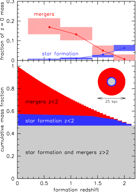
Figure 11.— Contribution of star formation and mergers at $0<z<2$ to the total stellar mass at $z=0$. The top panel shows the contributions of star formation (blue) and mergers (red) in each of our redshift bins. To calculate the blue points it was assumed that 50 % of the initial stellar mass is lost to winds. The contributions of mergers were calculated by subtracting the contributions of star formation from the total mass growth. The bottom panel shows the mass build-up over time due to star formation and mergers. The circles illustrate the mean effective radius of galaxies at $z=2$ (grey), $1.4<z<2$ (blue; star formation dominates), and $0<z<1.4$ (red; mergers dominate).

The contribution of mergers was calculated by subtracting the contribution of star formation from the total mass growth. In the highest redshift bin the contribution of mergers is very uncertain, but mergers at lower redshift contribute substantially to the $z=0$ mass. The growth rate due to mergers is consistent with a roughly constant value of $\sim 10$ ${\rm M}_{\odot}$ yr^-1 over the entire redshift range $0<z<2$. As the mass evolves by a factor of 2 since $z=2$, the “specific assembly rate” (i.e., the growth rate due to mergers divided by mass) actually increases with redshift by about a factor of 2. The merger rate can be parameterized as $dM/M=a(1+z)^{m}$, and we find $a\sim 0.03$ Gyr^-1 and $m\sim 1$ for our sample (see, e.g., Patton et al. 2002; Conselice et al. 2003, and many other studies).

As shown in the bottom panel of Fig. 11 some 40 % of the total stellar mass at $z=0$ was added through mergers at $0<z<2$. The circles in the bottom panel of Fig. 11 illustrate the increase in the effective radius from $z=2$ to $z=0$. Star formation dominates the growth at $1.5<z<2$ and may be responsible for the increase in $r_{e}$ over this redshift range. Mergers dominate at lower redshifts and are plausibly responsible for the size increase at $0<z<1.5$.

4.3. Color Gradients

If star formation dominates the growth of galaxies at $z=1.5-2$ and this growth mostly occurs at $r\gtrsim r_{e}$, one might expect that the galaxies exhibit significant color gradients at these redshifts. The gradients would be analogous to those in spiral galaxies, which usually have red bulges composed of old stars and blue disks with ongoing star formation. We measure color gradients by comparing surface brightness profiles of stacks in different bands. We only use the NMBS near-IR data as it is difficult to stack the optical CFHT images: the galaxies are typically very faint in the optical bands, and it is difficult to fully remove the light from the numerous blue galaxies in the field. We define a $J^{*}-K^{*}$ color, with $J^{*}=J_{1}+J_{2}$ and $K^{*}=H_{2}+K$. At $z=2$ this color roughly corresponds to rest-frame $U-R$.

Radial color profiles for the deconvolved stacks are shown in Fig. 12 (solid lines). The data are obviously noisy but show a clear trend: the galaxies are bluer with increasing radius at all redshifts. The errorbars are derived from bootstrapping the stacks and do not include systematic errors due to the deconvolution. Although some artifact in the deconvolution process may influence the results, the gradients are robust as the same trends are present in the original (convolved) stacks (dotted lines). As expected the stacked stellar image (see § 3.2; indicated by the black dotted line in Fig. 12) shows no appreciable trend with radius, demonstrating that the PSFs are well matched in the different bands. Although the color gradients are qualitatively consistent with the fact that blue galaxies at high redshift are larger than red galaxies (e.g., Toft et al. 2007; Zirm et al. 2007; Franx et al. 2008), it is not the same measurement: if the (large) blue and (small) red galaxies that enter our stacks had no color gradients we would not measure a gradient from the stack, as the images in each band are independently normalized.

There is an indication that the profiles steepen with redshift, with the $z=2.0$ stack having the largest color gradient. In the deconvolved stacks the rest-frame $U-R$ color at $r>5$ kpc is 0.5 – 1 mag bluer than the central color. This is a large difference, similar to that between red sequence and blue cloud galaxies in the nearby Universe (e.g., Ball, Loveday, & Brunner 2008). We infer that the color profiles are consistent with models in which massive galaxies at $z=1.5-2$ build up stellar mass at large radii through star formation. The averaged structure of massive galaxies at these redshifts appears to be qualitatively similar to nearby spiral galaxies, with a relatively old central component and a young disk. We note, however, that the galaxies that go into the stacks at these redshifts have a large range of properties. In particular, a significant fraction of the population is quiescent and compact (e.g., Cimatti et al. 2008; van Dokkum et al. 2008). A full description of massive galaxy evolution requires high quality data on large numbers of individual objects; so far, such data have only been collected for small samples (see, e.g., Genzel et al. 2006; Wright et al. 2009; Kriek et al. 2009b).

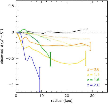
Figure 12.— Radial color profiles as a function of redshift, in observed $J_{*}-K_{*}$ (see text). The profiles were measured in the deconvolved stacks (solid lines) and in the original stacks (broken lines). Typical errorbars, derived from bootstrapping the stacks, are indicated at the end of each profile. The black broken line shows the profile of the stacked stellar image from $r=0\arcsec$ to $r=3\farcs 6$. The stacked galaxies become bluer with increasing radius, just like galaxies at $z=0$. The gradient is large at $z=2$, consistent with star formation occuring at large radii.

Irrespective of the physical cause of the observed gradients the immediate consequence is that the galaxies have gradients in $M/L$ ratio, such that the surface mass density for a given surface brightness is highest in the center (see de Jong 1996; Bell & de Jong 2001). The galaxies are therefore more compact in mass than in light. This is also the case at low redshift, as elliptical galaxies and spiral galaxies also have color gradients. However, the effect may be stronger at higher redshift, which would imply that the evolution in the mass-weighted effective radius is (even) stronger than in the luminosity-weighted radius. Several authors have suggested the opposite effect, i.e., that the sizes of high redshift galaxies may have been underestimated because of positive gradients in $M/L$ ratio. For example, in the models of Hopkins et al. (2009b) early-type galaxies form in mergers of spiral galaxies. Owing to star formation in the newly-forming core merger remnants have blue centers and red outer regions until $\gtrsim 0.5$ Gyr after the merger, when the color gradient starts to reverse. La Barbera & de Carvalho (2009) take this a step further, as they infer from color gradients of nearby galaxies that the apparent size evolution of massive galaxies can be entirely explained by a constant surface mass density profile combined with a strong radial age gradient. As noted above the actual effect is probably the opposite, which means that the evolution in Fig. 6 could be even stronger and the mass in the central 5 kpc (Fig. 9) may actually increase with redshift. However, given the large uncertainties we did not correct any of our results for gradients in $M/L$ ratio.

4.4. Implied Kinematics

As noted in many previous studies, high mass galaxies with relatively small effective radii are expected to have relatively high velocity dispersions, as the dispersion scales with $\sqrt{M/r_{e}}$ (e.g., Cimatti et al. 2008; van Dokkum et al. 2008; Franx et al. 2008; Bezanson et al. 2009). Velocity dispersions at high redshift provides constraints on the ratio of the stellar mass to the dynamical mass. Furthermore, as noted by, e.g., Hopkins et al. (2009c) and Cenarro & Trujillo (2009) the observed evolution of the velocity dispersion at fixed stellar mass may help distinguish between physical models for the size growth of massive galaxies.

It has been possible for some time to measure gas kinematics of star forming galaxies at high redshift (e.g., Pettini et al. 1998; Erb et al. 2003; Förster Schreiber et al. 2006). The interpretation is complicated by the fact that the gas disks are not always relaxed (e.g., Shapiro et al. 2008) and by the fact that massive star forming galaxies tend to be systematically larger than massive quiescent galaxies (e.g., Toft et al. 2007; Zirm et al. 2007). Quiescent galaxies generally lack strong emission lines, and their kinematics can only be measured from stellar absorption lines. Recently, the first such data have been obtained. Cenarro & Trujillo (2009) and Cappellari et al. (2009) measured velocity dispersions of compact galaxies at $z=1.5-2$, using deep optical spectroscopy. van Dokkum et al. (2009a) determined the velocity dispersion of a very small, high mass galaxy at $z=2.2$ from extremely deep near-IR spectroscopy. From these early results it appears that the observed dispersions are consistent with the measured sizes and masses. As an example from our own work, van Dokkum et al. (2008) predicted a velocity dispersion of $\sigma_{\rm predict}\sim 525$ km s^-1 for one of the most compact galaxies in their sample, and subsequently measured a dispersion of $\sigma_{\rm obs}=510^{+165}_{-95}$ km s^-1 (van Dokkum et al. 2009a). This also seems to hold at low redshift: Taylor et al. (2009) find that galaxies in SDSS that are more compact tend to have higher velocity dispersions, although we note that Trujillo et al. (2009) do not see the same trend in their analysis of SDSS daa.

So far, most studies have considered evolution of the velocity dispersion at fixed mass, which is obviously not the same as the actual evolution of the dispersion of any galaxy. Furthermore, the analysis is usually limited to quiescent galaxies. As noted by Franx et al. (2008); Hopkins et al. (2009c); Bezanson et al. (2009); Cenarro & Trujillo (2009) and others, a proper comparison would consider all progenitors, not just the quiescent galaxies, and explicitly take mass evolution into account. In the present study we independently measure the mass evolution and the size evolution at fixed number density, which allows us to predict the evolution of the velocity dispersion in a self-consistent way. We calculate the expected dispersion from the relation

$$M=r_{e}\langle\sigma^{2}\rangle\frac{s_{G}}{G},$$ (9)

where $M$ is the total mass, $\langle\sigma\rangle$ is the average line-of-sight velocity dispersion over the whole galaxy, weighted by luminosity, and $s_{G}$ is the dimensionless gravitational adius (see, e.g., Binney & Tremaine 1987; Djorgovski & Davis 1987; Ciotti 1991). As shown by Ciotti (1991) the gravitational radius is a (fairly weak) function of $n$, the Sersic index. A polynomial fit to the Ciotti (1991) numerical results,

$$s_{G}=3.316+0.026n-0.035n^{2}+0.00172n^{3},$$ (10)

is accurate to $<0.005$ dex over the range $n=2-10$.

The resulting redshift dependence of the luminosity-weighted line-of-sight velocity dispersion is shown in Fig. 13. The points are calculated from the observed $r_{e}$, $n$, and stellar mass at each redshift. The uncertainties are dominated by the uncertainty in the mass evolution. The solid line is the evolution that is implied by Eqs. 1, 4, and 5. The predicted dispersion increases with redshift by $\approx 0.1$ dex despite the fact that the masses decrease by a factor of $\approx 2$ over this redshift range. The reason for this counter-intuitive effect is that the effective radius decreases more rapidly with redshift than the mass.

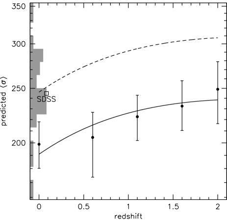
Figure 13.— Expected evolution of the mean luminosity-weighted velocity dispersion. Points and the solid line assume that $M_{\rm tot}=M_{\rm star}$, and should therefore be considered lower limits. The broken line has the same form as the solid line but is shifted to match the observed median velocity dispersions of SDSS galaxies (square) and $z=0$ elliptical galaxies (grey histogram; see Appendix D) with masses $\log M\sim 11.45$ ${\rm M}_{\odot}$. The mean velocity dispersion of galaxies with a number density of $n=2\times 10^{-4}$ Mpc^-3 is expected to increase with redshift, even though their masses decrease by a factor of $\sim 2$. Note that the scatter in $\log\sigma$ is expected to be considerable at each redshift.

The normalization of the curve is uncertain. The point labeled “SDSS” is the median dispersion of galaxies in SDSS with a median stellar mass of $\log M_{\rm star}=11.45$ in a $\pm 0.15$ dex bin (obtained from the NYU Value Added Galaxy Catalog; Blanton et al. 2005). The grey histogram shows the measured dispersions of the galaxies from the OBEY sample (Tal et al. 2009) that make up our $z=0$ stack (see Appendix D). The median dispersion is 245 km s^-1, very similar to the median dispersion of the SDSS galaxies. Note that there is a large range, with the highest value ($\sigma=342\pm 17$ km s^-1) measured for NGC 1399, the central galaxy in Fornax (Jørgensen, Franx, & Kjærgaard 1995). There are no data at higher redshift that can be used, as to our knowledge no kinematic studies of samples that are complete in stellar mass have been done. The measured $z=0$ dispersions are offset by $\approx 0.1$ dex from the predictions. This is not surprising as real galaxies have dark matter, gradients in $M/L$ ratio, and are not spherical. Furthermore, the SDSS and OBEY dispersions are measured in a fixed aperture (or corrected to the value at $r=0$), and are not identical to the luminosity-weighted mean dispersion. Scaling the predictions to match the $z=0$ data leads to a predicted median luminosity-weighted line-of-sight dispersion of $\sim 300$ km s^-1 at $z=2$. Hopkins et al. (2009c) suggest that the relative contributions of dark and luminous matter to the measured kinematics may be a function of redshift, which could change the evolution in Fig. 13. Cold gas may also contribute a non-negligible fraction of the mass at $z\sim 2$. We have also ignored the apparent evolution of color gradients (§ 4.3): the $z=2$ galaxies are very blue in the outer parts, and their (mass-weighted) effective radii are almost certainly significantly overestimated. Another complication is that the luminosity-weighted average dispersion is not necessarily the same as the measured dispersion within an aperture. Interestingly, high redshift data should be closer to this average than low redshift data as the aperture is larger in physical units at higher redshift.

Finally, we stress that the evolution in Fig. 13 is for complete samples of a given (evolving) mass. This includes star forming galaxies, which probably outnumber quiescent galaxies at $z=2$ (e.g., Papovich et al. 2006; Kriek et al. 2006). Star forming galaxies are larger than quiescent galaxies at a given mass and redshift (e.g., Trujillo et al. 2006; Toft et al. 2007; Zirm et al. 2007; Franx et al. 2008; Williams et al. 2009), and we can therefore expect the subset of quiescent galaxies at $z=2$ to have dispersions that are significantly larger than indicated in Fig. 13. Even within the sample of quiescent galaxies at $z\sim 2$ the scatter in size (and hence velocity dispersion) is substantial (e.g., Williams et al. 2009); as an example, the predicted velocity dispersions of the nine $z\approx 2.3$ galaxies in van Dokkum et al. (2008) range from $\sim 280$ km s^-1 to $\sim 540$ km s^-1. This is of course no different at $z=0$, as clearly indicated by the grey histogram in Fig. 13 (see also, e.g., Djorgovski & Davis 1987).

5. Summary and Conclusions

In this paper we study samples of galaxies at $0<z<2$ with a constant number density of $2\times 10^{-4}$ Mpc^-3. At low redshift galaxies with this number density have a stellar mass of $3\times 10^{11}$ ${\rm M}_{\odot}$ and live in halos of mean mass $\sim 5\times 10^{13}$ ${\rm M}_{\odot}$ (e.g., Wake et al. 2008; Brown et al. 2008), i.e., massive groups. They are mostly the central galaxies in these groups; only $\sim 10$ % are satellites (typically in clusters). This number-density selection is complementary to other selection techniques. The main advantage is that it allows a self-consistent comparison of galaxies at different redshifts, even if galaxies undergo mergers. High mass galaxies tend to merge with lower mass galaxies (see, e.g., Maller et al. 2006; Brown et al. 2007; Guo & White 2008, and Appendix A), which means that their number density remains roughly constant while their mass grows. The assumption is not that massive galaxies only evolve passively, but that a large fraction of the most massive galaxies at $z=0$ had at least one progenitor at higher redshift which was also among the most massive galaxies. An important drawback of this selection is that it can only be usefully applied to galaxies on the exponential tail of the mass function. A number density selection was previously applied by White et al. (2007), Brown et al. (2007, 2008), and Cool et al. (2008) to luminous red galaxies at $0.2<z<1$.

The stellar mass of galaxies with a number density $n=2\times 10^{-4}$ Mpc^-3 has evolved by a factor of $\approx 2$ since $z=2$. To our knowledge this is the first measurement of the mass evolution of the most massive galaxies over this redshift range. Previous studies have determined the evolution of the global mass density and the mass and number density down to fixed mass limits (e.g., Dickinson et al. 2003; Rudnick et al. 2003, 2006; Fontana et al. 2006; Pérez-González et al. 2008; Marchesini et al. 2009), but this is a subtly different measurement. On the exponential tail of the mass function the number density at fixed mass can change by factors of 5–10 for relatively small changes in mass. This complicates the interpretation of the evolution of the mass density, and also makes it highly susceptible to small errors in the masses (see also Brown et al. 2007). Nevertheless, we note that our results are consistent with previous studies of the mass function, and particularly with reports that the high mass end of the mass function does not show strong evolution (e.g., Fontana et al. 2006; Scarlata et al. 2007; Marchesini et al. 2009; Pozzetti et al. 2009). At lower redshifts we can compare our results to other work more directly. Brown et al. (2007) assessed the evolution of the most luminous red galaxies at $0<z<1$ in a similar way as is done in this study, namely by determining the evolution of the absolute magnitude of galaxies with a space density of $4.4\times 10^{-4}\,$Mpc^-3 (converted to our cosmology and to units of dex^-1 rather than mag^-1). Their sample selection does not include blue galaxies, but these are rare in this mass and redshift range. Using stellar population synthesis models to interpret the evolution of the absolute magnitude, Brown et al. (2007) find that $\approx 80$ % of the stellar mass of the most luminous red galaxies was already in place at $z=0.7$. This is almost exactly the mass evolution that we find here: Eq. 1 implies that 79 % of the mass is in place at $z=0.7$. It is also consistent with a later study by Cool et al. (2008) and it is qualitatively consistent with the evolution of the halo occupation distribution of red galaxies (White et al. 2007; Wake et al. 2008). Despite this consistency with other work systematic errors in the masses remain the largest cause for concern. As clearly demonstrated by Muzzin et al. (2009a, 2009b) these uncertainties cannot be addressed by obtaining deeper data or even (low resolution) continuum spectroscopy, as nearly identical model SEDs can have very different $M/L$ ratios.

The main result of our paper is that the mass growth of massive galaxies since $z=2$ is due to a gradual build-up of their outer envelopes. We find that the mass in the central regions is roughly constant with redshift, in qualitative agreement with results of Bezanson et al. (2009), Hopkins et al. (2009a), and Naab et al. (2009). From our analysis it appears that the well-known $r^{1/4}$ surface brightness profiles of elliptical galaxies are not the result of a sudden metamorphosis, like a caterpillar turning into a butterfly, but due to gradual evolution over the past 10 Gyr. We cannot be certain of this due to the limitations of our stacking technique: the evolution may appear more gradual than it really is if there is large scatter among the galaxies that enter the stacks. This is almost certainly the case at $z=2$ (e.g., Toft et al. 2007, Brammer et al. 2009). Figure 6 goes some way toward addressing a concern raised by Hopkins et al. (2009a), who suggest that observations may have missed the low surface brightness envelopes of normal elliptical galaxies at high redshift and that observers may have erroneously inferred small effective radii for galaxies at $z=1.5-2$. However, even deeper data at $z=2$ would be valuable to better constrain the form of the profiles at $r>15$ kpc. We note that van der Wel et al. (2008) already showed that surface brightness biases may exist in data of low S/N ratio but that they are likely small — and have the opposite sign for reasonable light profiles.

A direct consequence of the observed structural evolution is that massive galaxies do not evolve in a self-similar way. The structure of galaxies changes as a function of redshift, which means that the interpretation of scaling laws such as the fundamental plane (Djorgovski & Davis 1987; Dressler et al. 1987) also changes with redshift. This complicates many studies of the evolution of galaxies, as these usually either explicitly or implicitly assume self-similarity (e.g., Treu et al. 2005, van der Wel et al. 2006, van Dokkum & van der Marel 2007, Toft et al. 2007, Franx et al. 2008, Damjanov et al. 2009, Cenarro & Trujillo 2009, van Dokkum et al. 2009a, Cappellari et al. 2009, and many other studies). Dynamical modeling of spatially resolved internal kinematics and density profiles can take structural evolution explicitly into account. Interestingly, although there is no evidence for departures from simple virial relations in clusters at $z\approx 0.5$ (van der Marel & van Dokkum 2007), there are indications of such effects in rotationally supported field galaxies at $z\sim 1$ (van der Wel & van der Marel 2008).

From the star formation rates of galaxies that enter the stacks we infer that the physical mechanism that dominates the build-up of the outer regions since $z=1.5$ is likely some form of merging or accretion, consistent with many previous studies (e.g., van Dokkum et al. 1999; van Dokkum 2005; Tran et al. 2005; Bell et al. 2006; White et al. 2007; McIntosh et al. 2008; Naab et al. 2007, 2009). In-situ star formation may dominate the growth at $z=1.5-2$, but the newly formed stars account for only $\sim 10$ % of the total stellar mass at $z=0$ — about 1/4 of the contribution of mergers. The distinction between star formation and mergers is obviously somewhat diffuse at high redshift, as star forming disks may be continuously replenished (see, e.g., Genzel et al. 2008; Franx et al. 2008; Dekel et al. 2009). Furthermore, the galaxies that are accreted at $0<z<1$ may well have formed some fraction of their stars at $1<z<2$. It seems likely that star formation also dominated at $z>2$; as noted by many authors, the formation of the compact cores of elliptical galaxies was almost certainly a highly dissipative process (see, e.g., Kormendy et al. 2009, and references therein). It is unknown why star formation shuts off at later times; this could be due to feedback from an active nucleus (e.g., Croton et al. 2006; Bower et al. 2006), virial shock heating of the gas (e.g., Dekel & Birnboim 2006), gravitational heating due to accretion of gas or galaxies (e.g., Naab et al. 2007; Dekel & Birnboim 2008; Johansson, Naab, & Ostriker 2009), starvation (Cowie & Barger 2008), or other processes. Interestingly, we find that the shut-off is a rather sudden event, with the star formation rate dropping by a factor of 20 from $z=2$ to $z=1.1$ whereas the stellar mass grows only by a factor of 1.4 over this redshift range. This may suggest that the quenching trigger is not only a simple (stellar) mass threshold, as the range of masses in our selection bin is a factor of 2 at each redshift — larger than the evolution in the median mass. We note that the stellar mass threshold that we would derive is $\approx 2\times 10^{11}$ ${\rm M}_{\odot}$. Another open question is what the star formation histories are of the galaxies that are accreted (see, e.g., Naab et al. 2009). The properties of the stellar populations of elliptical galaxies at $r\gg r_{e}$ can give interesting constraints in this context (see, e.g., Weijmans et al. 2009).

The analysis in this paper can be improved and extended in many ways. The most obvious is to study the profiles of individual galaxies to large radii. Even though the stacking procedure should give reasonably accurate mean radii, the measured mean profile shape (parameterized by the Sersic $n$ parameter) can be in error (see Appendix B). Furthermore, valuable information is obviously lost — for example, the rich diversity of massive galaxies at $z\gtrsim 2$ (see Kriek et al. 2009b) — and the interpretation rests on several simplifying assumptions. The most important of these may be that all the galaxies that enter the stacks evolve in a somewhat homogenous way. It may well be that the samples consist of quite distinct populations whose relative number fractions change with time. We would interpret this as smooth evolution, whereas in reality there might be few individual galaxies that actually have the mean properties that we measure. Such effects are likely important at $z=1.5-2$ as our sample contains both quiescent and star forming galaxies at these redshifts, and they form quite distinct populations (e.g., Kriek et al. 2009b, Brammer et al. 2009). The population is likely more homogeneous at lower redshifts. At present studying surface brightness profiles of individual galaxies to very faint limits is only possible at low redshift (e.g., Kormendy et al. 2009, Tal et al. 2009), but progress can be expected from ongoing deep ground- and space-based surveys. We also assume that our samples are complete and unbiased at all redshifts, but there could be biases against very extended galaxies at the highest redshifts. We verified that individual galaxies with the properties of the $z=0.6$ stack would be detected (with approximately the correct flux) at $z=2$, but more extreme objects may have escaped detection. It will also be worthwhile to stack images with better spatial resolution. The highest redshift galaxies in our study are not resolved within the effective radius, and this may lead to biases in the Sersic fits.

One of the main uncertainties is the analysis is the conversion from rest-frame $R$ band light to mass. We know that the $M/L$ ratio is not constant with radius even at $z=0$, and we find good evidence for strong radial trends at higher redshift. It seems therefore possible that we might be overestimating the half-mass radii of galaxies at $z=2$ by a larger factor than we are overestimating the radii at $z=0$. We certainly do not see evidence for an an increasing $M/L$ ratio with radius, such as predicted by, among others, La Barbera & de Carvalho (2009). Upcoming surveys with WFC3 on HST will resolve this issue, and allow derivation of mass-weighted radii. Finally, we have mostly ignored the effects of dark matter in this paper, and of possible evolution in the IMF (e.g., van Dokkum 2008, Davé 2008, Wilkins et al. 2008). Kinematic data will give independent information on the masses of galaxies at high redshift, although it will be difficult to disentangle the effects of errors in stellar masses, changes in $s_{G}$, evolution in the stellar IMF, and the effects of dark matter. It will also be interesting to connect the evolution of these galaxies to the evolution of their halos, by combining the evolving stellar mass at fixed number density with clustering measurements and HOD modeling (see, e.g., White et al. 2007; Wake et al. 2008; Quadri et al. 2008).

Appendix A Appendix A. Effects of Mergers on the Mass Function

In this paper we select galaxies at a constant number density, as opposed to a constant luminosity or mass. At each redshift galaxies are selected in a narrow mass bin whose median mass corresponds to the mass appropriate for the chosen number density (see § 2.2). This selection is appropriate for processes that change the masses of galaxies and not their number densities, such as star formation and mass loss. However, mergers change both the mass and the number density of galaxies, and might be expected to complicate the selection. The effect of mergers on our selection was assessed with Monte Carlo simulations. A sample of 50,000 galaxies was created, distributed according to a Schechter (1976) mass function with characteristic mass $M_{*}\equiv 1$ and faint-end slope $\alpha=-1.2$, over the mass range $-1.5\leq\log(M/M_{*})\leq 1.0$. The simulation is independent of the precise value of $\alpha$; the value we chose is intermediate between two recent studies (Marchesini et al. 2009; Kajisawa et al. 2009). The left-most panel of Fig. 14 shows the high-mass end of this mass function. The horizontal line in this panel is an (arbitrarily chosen) constant number density of $n_{\rm sel}=32$ galaxies per bin. The red histogram shows galaxies with masses in the range $0.2\leq\log(M/M_{*})\leq 0.5$.

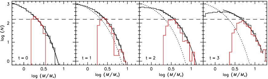
Figure 14.— Monte-Carlo simulation demonstrating the effects of merging on our constant-number density selection. At $t=0$ galaxies are distributed according to a Schechter (1976) function (dotted line in each panel). At each timestep, all galaxies merge with one other galaxy, reducing the total number density by a factor of 2. The mass ratio of the mergers is randomly chosen between $1:10$ and $1:2$. The dashed horizontal line is a line of constant number density. The red histograms show galaxies with initial masses of $0.2\leq\log(M/M_{*})\leq 0.5$ and their descendants. Because of the steepness of the mass function at $M>M_{*}$ the descendants have roughly the same number density as their progenitors.

From time step $t=0$ to $t=1$ all galaxies are merged with each other, reducing the total number of galaxies by a factor of two. Mergers of galaxies with mass ratios between $1:10$ and $1:2$ have equal probability. The results are qualitatively similar if other limits are assumed, such as a constant $1:4$ ratio. The red histogram at $t=1$ shows the distribution of galaxies that have at least one progenitor whose original mass was in the range $0.2\leq\log(M/M_{*})\leq 0.5$. The distribution is shifted and has broadened, but the median mass is very similar to the mass of galaxies with a number density of $n_{\rm sel}$. Similarly, the merger remnants are merged with each other from $t=1$ to $t=2$ and again from $t=2$ to $t=3$.

We applied the same selection method as used in § 2.2 to the simulated sample. Exponential functions were fit to the high mass end of the mass function (solid lines in Fig. 14), and the intersections of these lines with $n_{\rm sel}$ (horizontal dashed lines) were determined. The left panel of Fig. 15 compares the actual median masses of all descendants of galaxies with $0.2\leq\log(M/M_{*})\leq 0.5$ at $t=0$ to the measured masses at fixed number density. There is excellent agreement, demonstrating that our selection method gives the correct mass evolution for a merging population of galaxies. Next, we selected galaxies in a mass bin of width $\pm 0.15$ dex centered on the evolving mass. These bins miss some of the descendants as their mass distribution broadens with time. The middle panel of Fig. 15 shows the fraction of actual descendants that are contained within the selection bin. This fraction is $\sim 70$ % for mass evolution of a factor of two. Finally, the right panel shows the fraction of galaxies in the bin that are not descendants of galaxies with original masses $0.2\leq\log(M/M_{*})\leq 0.5$. This fraction is $\sim 40$ % for a factor of two mass evolution, but we note that all of these galaxies had original masses close to the selected range.

Figure 15.— Results from the Monte Carlo simulation. Left panel: Comparison of the actual median mass of the descendants of galaxies with initial masses $0.2\leq\log(M/M_{*})\leq 0.5$ to the measured mass at fixed number density (which is used in this paper). There is excellent agreement. The double arrow indicates the range of masses measured at $0<z<2$ (see § 2.2). Middle panel: Fraction of descendants that is selected with the method described in § 2.2. Right panel: Fraction of galaxies that are selected but are not descendants. Over the relevant mass range the completeness is high and the contamination low.

In summary, a selection at constant number density should give a fairly homogeneous sample of galaxies as a function of redshift. Mass evolution can be measured directly in a self-consistent way, regardless of the physical process (star formation or mergers). In reality mergers likely dominate at the high-mass end of the mass function and star formation likely dominates at the low-mass end (e.g., Guo & White 2008; Damen et al. 2009). We note that our simple simulation demonstrates that the observed average mass growth of a factor of two at high masses can be explained by three mergers with random mass ratio between $1:10$ and $1:2$. The selection does not produce homogeneous samples if growth occurs through $1:1$ mergers only (and no other mergers), but that is exceedingly unlikely (see, e.g., van Dokkum 2005; Naab et al. 2007; Guo & White 2008).

Appendix B Appendix B. Recovering Average Structural Parameters from Stacked Images

A key aspect of this study is that structural parameters are not measured from individual images and then averaged but measured from averaged images of many individual galaxies. We tested how well the structural parameters $r_{e}$ and $n$ can be recovered with this method by creating stacks of simulated galaxies and by analyzing real galaxies.

B.1. Model galaxies

Model galaxies were created with GALFIT (Peng et al. 2002). Their Sersic indices are distributed randomly between $n=1$ and $n=4$, their axis ratios range from $b/a=0.1$ to $b/a=1.0$, and they have random position angles. The results are not sensitive to the assumed distribution of $n$ or $b/a$. Ten stacks were created of 200 galaxies each. The ten stacks differ in their distributions of circularized effective radii. The radii were chosen randomly within the range $0.5r_{n}<r_{e}<2r_{n}$, with $r_{n}$ ranging from $r_{1}=1$ kpc to $r_{10}=10$ kpc. Prior to stacking the galaxies were placed at $z=2$, convolved with a Moffat PSF with a FWHM of $1\farcs 1$, and sampled with $0\farcs 3$ pixels.

The stacked images were fit with GALFIT and the results are shown in Fig. 16 (black lines). The circularized effective radii are recovered well, even for $\langle r_{e}\rangle=1-2$ kpc. This is remarkable as these scales correspond to $0\farcs 1-0\farcs 2$, a small fraction of the FWHM of the PSF. Broken lines and solid lines are for two different ways of averaging the effective radii of individual galaxies: solid lines show averages of $\log r_{e}$ and broken lines are for the logarithm of the average $r_{e}$. The stacks clearly measure the average of $r_{e}$ rather than the average of $\log r_{e}$ but the differences are small. The right panel shows how well the average Sersic index is recovered. The stacks systematically overestimate the Sersic index. This can be understood by considering the average profile of a small galaxy and a large galaxy, both with $n=1$. The small galaxy will add a peak at small radii to the extended profile of the large galaxy, creating a profile best fit by a model with larger $n$.

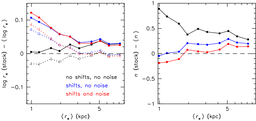
Figure 16.— Left panel: Comparison of the effective radius as measured from a stack of 200 galaxies to the mean circularized effective radius of the individual galaxies. Black is for a noiseless stack, blue is for a noiseless stack with Gaussian 0.25 pixel shifts applied to the individual galaxies, and red is for a stack with shifts and the same noise as the $z=2$ stack of real galaxies. Solid lines show results for $\langle\log r_{e}\rangle$ and broken lines are for $\log\langle r_{e}\rangle$. Sizes $\gtrsim 2$ kpc can be measured fairly reliably, with a systematic error of $\sim 10$ %. Right panel: Comparison of Sersic (1968) index $n$. The stacks tend to overestimate the true average Sersic index, by $\lesssim 0.5$. Note that stacks with simulated shifts and noise perform better than noiseless stacks.

The noiseless test is useful as it demonstrates that the stacking technique can give results that can be compared directly with measurements of individual galaxies. However, in order to assess the systematic errors associated with our methodology centroiding errors and noise need to be taken into account. Centroiding errors were simulated by shifting the individual images by small amounts, using the same third order polynomial interpolation as was used for the real data. The shifts were drawn from a Gaussian distribution with $\sigma=0.25$ pixels (2.1 kpc). Blue curves in Fig. 16 show the effects of these shifts on the recovered parameters. As expected, the smoothing leads to an overestimate of the effective radius. However, the effect is fairly small because the profiles at larger radii are not strongly affected by the centroiding errors. The average Sersic parameter is actually better determined when small shifts are included, probably because the central peak (caused by galaxies with small $r_{e}$) is smeared out in the stacks.

Finally, noise was added to the modeled stacks. A noise image was created from the actual residual map of the $z=2$ stack, thus ensuring that the noise level, correlations between pixels, and non-Gaussian components are all exactly identical to the actual data. The $z=2$ stack has the highest noise of our four stacks as the galaxies are fainter than those at lower redshift. The noise images were added to the artificial stacks, and structural parameters were remeasured. The red curves in Fig. 16 show the results. They are quite similar to the blue curves, suggesting that systematic effects dominate over the effects of noise. In summary, we should be able to determine effective radii and Sersic $n$ parameters with reasonable accuracy despite the poor spatial resolution of our data, if the surface brightness profiles are well described by Sersic fits.

Figure 17.— Comparison of the effective radius and Sersic $n$ parameters of individual galaxies in the $z=0$ OBEY sample to the average as measured from the stacked image. The results from the stack are indicated by the solid circle with errorbars. The actual means of the individual galaxies are indicated with the cross. The measurements from the stack are fully consistent with the means of the individual galaxies.

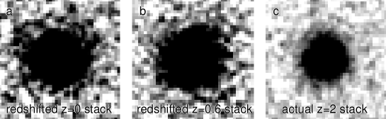
Figure 18.— a) Stack of $z=0$ OBEY galaxies redshifted to $z=2$; b) stack of $z=0.6$ NMBS galaxies redshifted to $z=2$; and c) stack of actual NMBS $z=2$ galaxies. The images span $12^{\prime\prime}\times 12^{\prime\prime}$, and are normalized by the peak flux. The contrast is scaled to bring out differences in the outer regions. The redshifted low redshift stacks are more extended than the $z=2$ stack, showing low surface brightness emission out to large radii.

B.2. Real galaxies

Real galaxies do not necessarily follow Sersic profiles, and subtle deviations for individual galaxies may lead to significant systematic differences when determining structural parameters from stacked data. We first test whether the structural parameters that we derive for the stacked $z=0$ OBEY sample (see Appendix D) are consistent with the average of the individual galaxies. We fitted Sersic (1968) profiles and determined circularized effective radii in kpc and the Sersic $n$ parameter for each of the 14 galaxies that enter the OBEY stack. The results are shown in Fig. 17. We find $\langle r_{e}\rangle=12.6$ kpc and $\langle n\rangle=6.4$. The structural parameters measured from the stacked image are very similar at $r_{e}=12.4^{+1.6}_{-1.3}$ kpc, $n=5.9^{+0.7}_{-0.6}$, and we conclude that the stacking method gives reasonable results for real galaxies.

Next, we assess the importance of redshift-dependent effects by redshifting the $z=0$ OBEY stack and the $z=0.6$ NMBS stack to $z=2$. The angular scale and fluxes of the profiles of the OBEY galaxies were corrected to $z=2$, the galaxies were convolved with the NMBS PSF, the images were resampled to match the NMBS resolution of $0\farcs 3$ pixel^-1, and empirical noise derived from empty regions of the actual NMBS images was added. The $z=0.6$ images were only scaled in flux, as they have a similar PSF and spatial scale as the $z=2$ images. Noise was added in the same way as for the OBEY stack.

The resulting redshifted images are shown in Fig. 18, along with the actual $z=2$ stack. To highlight the differences in profile shape the images were normalized to the peak flux. It is clear that the actual $z=2$ image is more compact than the redshifted $z=0$ and $z=0.6$ stacks, as it lacks the low surface brightness features that surround the bright cores in the lower redshift stacks. We quantified the effects of redshifting by fitting Sersic profiles to the redshifted stacks. The redshifted OBEY stack gives $r_{e}=11.0$ kpc and $n=4.9$, in good agreement with the original values ($r_{e}=12.4^{+1.6}_{-1.3}$ kpc, $n=5.9^{+0.7}_{-0.6}$). The redshifted $z=0.6$ stack gives $r_{e}=8.0$ kpc and $n=4.4$, again in good agreement with the original values ($r_{e}=8.0^{+1.2}_{-0.5}$ kpc, $n=4.0^{+0.4}_{-0.4}$). From these tests we conclude that there are no obvious redshift-dependent effects which could lead to severe biases in the derived evolution.

Appendix C Appendix C. Individual Galaxy Images

Here we show the individual images of galaxies that enter the stacks.

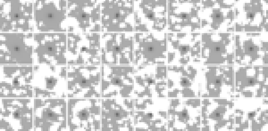
Figure 19.— The 32 galaxies with $\log M\approx 11.36$ and $0.2<z<0.8$ that enter the $\langle z\rangle=0.6$ stack. The images are averages of $J_{1}$ and $J_{2}$. Masked regions are white. Each image was normalized using the summed flux in the central $10\times 10$ pixels ($3\farcs 0\times 3\farcs 0$); this is why the background noise is not the same for all galaxies. Note: Figures C1-C4 were degraded to adhere to arXiv’s file size limits.

Figure 20.— The 87 galaxies with $\log M\approx 11.28$ and $0.8<z<1.4$ that enter the $\langle z\rangle=1.1$ stack. The images are averages of $J_{3}$ and $H_{1}$.

Figure 21.— The 73 galaxies with $\log M\approx 11.21$ and $1.4<z<1.8$ that enter the $\langle z\rangle=1.6$ stack. The images are averages of $H_{1}$ and $H_{2}$.

Figure 22.— The 78 galaxies with $\log M\approx 11.15$ and $1.8<z<2.2$ that enter the $\langle z\rangle=2.0$ stack. The images are averages of $H_{2}$ and $K$.

Appendix D Appendix D. Low Redshift Galaxies

D.1. The OBEY Sample

The data over the redshift range $0.6<z<2.0$ are analyzed in a self-consistent way, and are all drawn from the same survey (the NEWFIRM Medium Band Survey, or NMBS). Although essentially all the results presented in this paper could be derived from the NMBS data alone, we made some effort to construct a $z=0$ sample that can be analyzed in the same way as the data at higher redshift. Key requirements are that the masses are on the same system as the high $z$ data and that very deep photometry is available to probe the faint outer regions of the galaxies. We use data from a recent public survey of luminous elliptical galaxies, called Observations of Bright Ellipticals at Yale (OBEY) (Tal et al. 2009). The OBEY sample consists of all elliptical galaxies from the Tully (1988) Nearby Galaxies Catalog with distances 15 – 50 Mpc, luminosities $M_{B}<-20$, declinations between $-85^{\circ}$ and $+10^{\circ}$, and Galactic latitude $>17^{\circ}$. The galaxies were observed with the CTIO 1 m telescope, as described in Tal et al. (2009). Owing to very careful flatfielding the surface brightness profiles can be reliably traced to large radii. The data are publicly available.

We determined stellar masses for the galaxies in the OBEY sample in the following way. Total magnitudes and colors were obtained from Prugniel & Heraudeau (1998) through the HyperLeda interface (Paturel et al. 2003). The “extrapolated” total $B$ magnitudes were used together with “effective” luminosity-weighted $U-B$, $B-V$, $V-R$, and $V-I$ colors to create $UBVRI$ SEDs. The apparent magnitudes were corrected for Galactic extinction using the estimates from Schlegel, Finkbeiner, & Davis (1998) and converted to absolute magnitudes using the distances given in Tully (1988) (corrected to our cosmology). Stellar masses were determined using FAST (Kriek et al. 2009a), a code that fits stellar population synthesis models to observed photometry. This code was also used to determine the stellar masses of the galaxies in the NMBS, and we used the same stellar population synthesis model, dust law, and other parameters as were used for the fits to the distant galaxies (see § 2.1). The only difference is that we fixed the value of the characteristic star formation timescale $\tau$ to 1 Gyr. If $\tau$, age, and $A_{V}$ are all free parameters the fits show aliasing due to the limited number of data points. We verified that this small change to the fitting procedure does not lead to systematic biases in the masses.

The relation between stellar mass and total absolute $B$ magnitude is shown in Fig. 23. Solid symbols are galaxies in the OBEY sample. Open symbols are galaxies with $M_{B}^{T}\lesssim-21$ in the Tully (1988) catalog that are not classified as elliptical galaxies, and therefore not in the OBEY sample. We note that for one of these galaxies we adopted a different distance than is listed in the Tully (1988) atlas: for NGC 4594 (M104) we used a distance of 9.1 Mpc (Jensen et al. 2003) rather than 21 Mpc. The grey band indicates the same selection as was used at higher redshift: a mass bin of width $\pm 0.15$ dex and median mass determined by Eq. 1 ($\log M_{n}=11.45$ for $z=0$). This bin contains 14 elliptical galaxies from the OBEY sample: NGC 1399, NGC 1407, NGC 2986, IC 3370, NGC 3585, NGC 3706, NGC 4697, NGC 4767, NGC 5044, NGC 5077, NGC 5813, NGC 5846, NGC 6861, and NGC 6868.

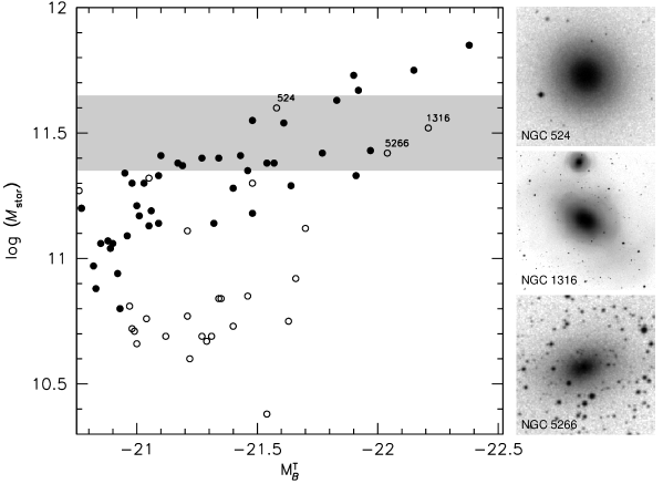
Figure 23.— Relation between stellar mass and total absolute $B$ magnitude for elliptical galaxies in the OBEY sample (solid points) and other bright galaxies in the same volume (open symbols). The grey band indicates our selection: a $\pm 0.15$ dex band containing galaxies with a median mass of $\log M_{n}=11.45$. Most galaxies in this mass range are in the OBEY sample. The only exceptions are NGC 524, NGC 1316, and NGC 5266 as all three are classified as S0 in Tully (1988). However, all three galaxies have large bulges and presumably similar surface brightness profiles as the other 14 galaxies in this mass bin.

Only three galaxies have masses near $M_{n}$ but are not in the OBEY sample: NGC 524, NGC 1316, and NGC 5266. All three are classified as S0 in the Tully (1988) atlas. NGC 524 is a face-on S0, but it has a velocity dispersion of 235 km s^-1 and an effective radius of 9 kpc (Emsellem et al. 2007) — close to the average $r_{e}$ of the OBEY stack. NGC 1316 is the well-known radio galaxy Fornax A. It is a merger remnant with striking dust lanes (Schweizer 1980) and significant mid-IR emission (Temi, Mathews, & Brighenti 2005). Its effective radius is $\approx 8$ kpc (e.g., Temi et al. 2005), although this may be an underestimate as the galaxy has a large halo of diffuse light (e.g., Schweizer 1980). NGC 5266 has a prominent dust lane, but can otherwise be considered an elliptical galaxy (e.g., Varnas et al. 1987). In summary, although the OBEY sample is not a mass-limited sample, it misses less than 20 % of galaxies in the relevant mass range and there is no indication that the galaxies that are missed have different surface density profiles from the OBEY galaxies.

An average stack was created from the 14 OBEY galaxies. Rather than averaging the galaxies themselves we averaged the 2D surface brightness distributions that were measured by Tal et al. (2009). These model images are excellent representations of the galaxies and avoid contamination from the many neighboring stars and galaxies. Each galaxy was normalized to the flux inside a 24 kpc $\times$ 24 kpc region centered on the galaxy (equivalent to the $10\times 10$ pixel box used at higher redshift). After averaging the galaxies the flux outside $r=75$ kpc was set to zero and the total mass was normalized according to Eq. 2.

For the analysis in § 4.4 velocity dispersions of the OBEY galaxies were obtained from the literature, using the Leda database. They come from a variety of sources; when multiple measurements were available we preferentially used data from Faber et al. (1989), Franx, Illingworth, & Heckman (1989), or Jørgensen et al. (1995). They are indicative only as they are not necessarily measured in a homogeneous way and do not necessarily correspond to the same physical aperture.

D.2. Comparison to Other Studies

Here we briefly compare our datapoint at $z=0$ from the OBEY sample to results from other recent studies. Shen et al. (2003) determined the mass-size relation for early-type galaxies from SDSS data, using masses from Kauffmann et al. (2003a) and sizes from Blanton et al. (2003). Their relation is shown by the dashed line in Fig. 24. Grey points are individual galaxies taken from the NYU Value Added Galaxy Catalog (NYU-VACG) website (Blanton et al. 2005). They are in good agreement with the Shen et al. relation, as expected. The solid line shows the relation obtained by Guo et al. (2009) for SDSS early-type galaxies. These authors find a significantly steeper relation then Shen et al. (2003), possibly because Blanton et al. (2003) underestimated both the size and the luminosity of bright galaxies. As implied by Eq. 7 (and as shown in Appendix A of Guo et al. 2009) errors in $r_{e}$ can be much larger than errors in the total luminosity, if flux is missed at large radii.

Figure 24.— Comparison of mass-size relations at $z=0$. Grey points (not shown in arXiv version due to file size restrictions) are data from Blanton et al. (2003) and Kauffmann et al. (2003). The dashed line is the fit from Shen et al. (2003) to early-type galaxies, based on these data. Guo et al. (2009) infer that Blanton et al. underestimated the sizes of massive galaxies, and find a steeper relation. Open squares are elliptical galaxies in Virgo, whose sizes were measured by Kormendy et al. (2009). The solid square is our measurement from the OBEY sample.

We also compare our datapoint to data for individual galaxies in the Virgo cluster. Kormendy et al. (2009) determined effective radii of elliptical galaxies in Virgo by integrating their surface brightness profiles, using very deep and homogeneous data. These are arguably the most accurate half-light radii for elliptical galaxies yet measured. We determined masses for the galaxies in the Kormendy et al. (2009) sample in the same way as was done for the OBEY sample. Open squares in Fig. 24 indicate the masses and sizes of the Virgo ellipticals.

The OBEY point falls very close to the relation of Guo et al. (2009) and to the four Virgo elliptical galaxies that have masses near $3\times 10^{11}$ ${\rm M}_{\odot}$. The average values for these four galaxies are plotted in Fig. 8 in the main text of the paper. The difference between the Guo et al. relation and the OBEY point can easily be explained by a $0.05-0.1$ systematic difference in $\log M$ or sample variance, as the difference is only slightly more than $1\sigma$.

References

- (1)
- (2) Ball, N. M., Loveday, J., & Brunner, R. J. 2008, MNRAS, 383, 907
- (3)
- (4) Barmby, P., Alonso-Herrero, A., Donley, J. L., Egami, E., Fazio, G. G., Georgakakis, A., Huang, J.-S., Laird, E. S., et al. 2006, ApJ, 642, 126
- (5)
- (6) Bell, E. F. & de Jong, R. S. 2001, ApJ, 550, 212
- (7)
- (8) Bell, E. F., Naab, T., McIntosh, D. H., Somerville, R. S., Caldwell, J. A. R., Barden, M., Wolf, C., Rix, H.-W., et al. 2006, ApJ, 640, 241
- (9)
- (10) Bell, E. F., Wolf, C., Meisenheimer, K., Rix, H., Borch, A., Dye, S., Kleinheinrich, M., Wisotzki, L., et al. 2004, ApJ, 608, 752
- (11)
- (12) Bertin, E., & Arnouts, S. 1996, A&AS, 117, 393
- (13)
- (14) Bezanson, R., van Dokkum, P. G., Tal, T., Marchesini, D., Kriek, M., Franx, M., & Coppi, P. 2009, ApJ, 697, 1290
- (15)
- (16) Binney, J. & Tremaine, S. 1987, Galactic dynamics, ed. J. Binney & S. Tremaine
- (17)
- (18) Blanton, M. R., Hogg, D. W., Bahcall, N. A., Baldry, I. K., Brinkmann, J., Csabai, I., Eisenstein, D., Fukugita, M., et al. 2003, ApJ, 594, 186
- (19)
- (20) Blanton, M. R., Schlegel, D. J., Strauss, M. A., Brinkmann, J., Finkbeiner, D., Fukugita, M., Gunn, J. E., Hogg, D. W., et al. 2005, AJ, 129, 2562
- (21)
- (22) Bower, R. G., Benson, A. J., Malbon, R., Helly, J. C., Frenk, C. S., Baugh, C. M., Cole, S., & Lacey, C. G. 2006, MNRAS, 370, 645
- (23)
- (24) Brammer, G. B., van Dokkum, P. G., & Coppi, P. 2008, ApJ, 686, 1503
- (25)
- (26) Brammer, G. B., Whitaker, K. E., van Dokkum, P. G., Marchesini, D., Labbé, I., Franx, M., Kriek, M., Quadri, R. F., et al. 2009, ApJ Letters, submitted
- (27)
- (28) Brown, M. J. I., Dey, A., Jannuzi, B. T., Brand, K., Benson, A. J., Brodwin, M., Croton, D. J., & Eisenhardt, P. R. 2007, ApJ, 654, 858
- (29)
- (30) Brown, M. J. I., Zheng, Z., White, M., Dey, A., Jannuzi, B. T., Benson, A. J., Brand, K., Brodwin, M., et al. 2008, ApJ, 682, 937
- (31)
- (32) Buitrago, F., Trujillo, I., Conselice, C. J., Bouwens, R. J., Dickinson, M., & Yan, H. 2008, ApJ, 687, L61
- (33)
- (34) Calzetti, D., Armus, L., Bohlin, R. C., Kinney, A. L., Koornneef, J., & Storchi-Bergmann, T. 2000, ApJ, 533, 682
- (35)
- (36) Cappellari, M., di Serego Alighieri, S., Cimatti, A., Daddi, E., Renzini, A., Kurk, J. D., Cassata, P., Dickinson, M., et al. 2009, ApJ Letters, submitted (arXiv:0906.3648)
- (37)
- (38) Cenarro, A. J. & Trujillo, I. 2009, ApJ, 696, L43
- (39)
- (40) Cimatti, A., Cassata, P., Pozzetti, L., Kurk, J., Mignoli, M., Renzini, A., Daddi, E., Bolzonella, M., et al. 2008, A&A, 482, 21
- (41)
- (42) Ciotti, L. 1991, A&A, 249, 99
- (43)
- (44) Cole, S., Norberg, P., Baugh, C. M., Frenk, C. S., Bland-Hawthorn, J., Bridges, T., Cannon, R., Colless, M., et al. 2001, MNRAS, 326, 255
- (45)
- (46) Conselice, C. J., Bershady, M. A., Dickinson, M., & Papovich, C. 2003, AJ, 126, 1183
- (47)
- (48) Cool, R. J., Eisenstein, D. J., Fan, X., Fukugita, M., Jiang, L., Maraston, C., Meiksin, A., Schneider, D. P., et al. 2008, ApJ, 682, 919
- (49)
- (50) Cowie, L. L. & Barger, A. J. 2008, ApJ, 686, 72
- (51)
- (52) Croton, D. J., Springel, V., White, S. D. M., De Lucia, G., Frenk, C. S., Gao, L., Jenkins, A., Kauffmann, G., et al. 2006, MNRAS, 365, 11
- (53)
- (54) Daddi, E., Renzini, A., Pirzkal, N., Cimatti, A., Malhotra, S., Stiavelli, M., Xu, C., Pasquali, A., et al. 2005, ApJ, 626, 680
- (55)
- (56) Damen, M., Labbé, I., Franx, M., van Dokkum, P. G., Taylor, E. N., & Gawiser, E. J. 2009, ApJ, 690, 937
- (57)
- (58) Damjanov, I., McCarthy, P. J., Abraham, R. G., Glazebrook, K., Yan, H., Mentuch, E., LeBorgne, D., Savaglio, S., et al. 2009, ApJ, 695, 101
- (59)
- (60) Davé, R. 2008, MNRAS, 385, 147
- (61)
- (62) Davis, M., Guhathakurta, P., Konidaris, N. P., Newman, J. A., Ashby, M. L. N., Biggs, A. D., Barmby, P., Bundy, K., et al. 2007, ApJ, 660, L1
- (63)
- (64) de Jong, R. S. 1996, A&A, 313, 377
- (65)
- (66) De Lucia, G., Springel, V., White, S. D. M., Croton, D., & Kauffmann, G. 2006, MNRAS, 366, 499
- (67)
- (68) Dekel, A. & Birnboim, Y. 2006, MNRAS, 368, 2
- (69)
- (70) —. 2008, MNRAS, 383, 119
- (71)
- (72) Dekel, A., Birnboim, Y., Engel, G., Freundlich, J., Goerdt, T., Mumcuoglu, M., Neistein, E., Pichon, C., et al. 2009, Nature, 457, 451
- (73)
- (74) Dickinson, M., Papovich, C., Ferguson, H. C., & Budavári, T. 2003, ApJ, 587, 25
- (75)
- (76) Djorgovski, S. & Davis, M. 1987, ApJ, 313, 59
- (77)
- (78) Dressler, A., Lynden-Bell, D., Burstein, D., Davies, R. L., Faber, S. M., Terlevich, R., & Wegner, G. 1987, ApJ, 313, 42
- (79)
- (80) Drory, N., Bender, R., & Hopp, U. 2004, ApJ, 616, L103
- (81)
- (82) Dunkley, J., Komatsu, E., Nolta, M. R., Spergel, D. N., Larson, D., Hinshaw, G., Page, L., Bennett, C. L., et al. 2009, ApJS, 180, 306
- (83)
- (84) Emsellem, E., Cappellari, M., Krajnović, D., van de Ven, G., Bacon, R., Bureau, M., Davies, R. L., de Zeeuw, P. T., et al. 2007, MNRAS, 379, 401
- (85)
- (86) Erb, D. K., Shapley, A. E., Steidel, C. C., Pettini, M., Adelberger, K. L., Hunt, M. P., Moorwood, A. F. M., & Cuby, J. 2003, ApJ, 591, 101
- (87)
- (88) Erben, T., Hildebrandt, H., Lerchster, M., Hudelot, P., Benjamin, J., van Waerbeke, L., Schrabback, T., Brimioulle, F., et al. 2009, A&A, 493, 1197
- (89)
- (90) Faber, S. M., Wegner, G., Burstein, D., Davies, R. L., Dressler, A., Lynden-Bell, D., & Terlevich, R. J. 1989, ApJS, 69, 763
- (91)
- (92) Faber, S. M., Willmer, C. N. A., Wolf, C., Koo, D. C., Weiner, B. J., Newman, J. A., Im, M., Coil, A. L., et al. 2007, ApJ, 665, 265
- (93)
- (94) Fan, L., Lapi, A., De Zotti, G., & Danese, L. 2008, ApJ, 689, L101
- (95)
- (96) Fontana, A., Salimbeni, S., Grazian, A., Giallongo, E., Pentericci, L., Nonino, M., Fontanot, F., Menci, N., et al. 2006, A&A, 459, 745
- (97)
- (98) Förster Schreiber, N. M., Genzel, R., Lehnert, M. D., Bouché, N., Verma, A., Erb, D. K., Shapley, A. E., Steidel, C. C., et al. 2006, ApJ, 645, 1062
- (99)
- (100) Franx, M., Illingworth, G., & Heckman, T. 1989, ApJ, 344, 613
- (101)
- (102) Franx, M., van Dokkum, P. G., Schreiber, N. M. F., Wuyts, S., Labbé, I., & Toft, S. 2008, ApJ, 688, 770
- (103)
- (104) Gargiulo, A., Haines, C. P., Merluzzi, P., Smith, R. J., Barbera, F. L., Busarello, G., Lucey, J. R., Mercurio, A., et al. 2009, MNRAS, 805
- (105)
- (106) Gebhardt, K., Lauer, T. R., Pinkney, J., Bender, R., Richstone, D., Aller, M., Bower, G., Dressler, A., et al. 2007, ApJ, 671, 1321
- (107)
- (108) Genzel, R., Burkert, A., Bouché, N., Cresci, G., Förster Schreiber, N. M., Shapley, A., Shapiro, K., Tacconi, L. J., et al. 2008, ApJ, 687, 59
- (109)
- (110) Genzel, R., Tacconi, L. J., Eisenhauer, F., Förster Schreiber, N. M., Cimatti, A., Daddi, E., Bouché, N., Davies, R., et al. 2006, Nature, 442, 786
- (111)
- (112) Griffiths, R. E., Ratnatunga, K. U., Neuschaefer, L. W., Casertano, S., Im, M., Wyckoff, E. W., Ellis, R. S., Gilmore, G. F., et al. 1994, ApJ, 437, 67
- (113)
- (114) Guo, Q. & White, S. D. M. 2008, MNRAS, 384, 2
- (115)
- (116) Guo, Y., McIntosh, D. H., Mo, H. J., Katz, N., van den Bosch, F. C., Weinberg, M., Weinmann, S. M., Pasqual, A., et al. 2009, MNRAS, in press (arXiv:0901.1150)
- (117)
- (118) Hildebrandt, H., Pielorz, J., Erben, T., van Waerbeke, L., Simon, P., & Capak, P. 2009, A&A, 498, 725
- (119)
- (120) Högbom, J. A. 1974, A&AS, 15, 417
- (121)
- (122) Holden, B. P., Stanford, S. A., Eisenhardt, P., & Dickinson, M. 2004, AJ, 127, 2484
- (123)
- (124) Hopkins, P. F., Bundy, K., Murray, N., Quataert, E., Lauer, T. R., & Ma, C.-P. 2009a, MNRAS, 1043
- (125)
- (126) Hopkins, P. F., Cox, T. J., Dutta, S. N., Hernquist, L., Kormendy, J., & Lauer, T. R. 2009b, ApJS, 181, 135
- (127)
- (128) Hopkins, P. F., Hernquist, L., Cox, T. J., Keres, D., & Wuyts, S. 2009c, ApJ, 691, 1424
- (129)
- (130) Hyde, J. B. & Bernardi, M. 2009, MNRAS, 396, 1171
- (131)
- (132) Ilbert, O., Capak, P., Salvato, M., Aussel, H., McCracken, H. J., Sanders, D. B., Scoville, N., Kartaltepe, J., et al. 2009, ApJ, 690, 1236
- (133)
- (134) Jensen, J. B., Tonry, J. L., Barris, B. J., Thompson, R. I., Liu, M. C., Rieke, M. J., Ajhar, E. A., & Blakeslee, J. P. 2003, ApJ, 583, 712
- (135)
- (136) Johansson, P. H., Naab, T., & Ostriker, J. P. 2009, ApJ, 697, L38
- (137)
- (138) Jørgensen, I., Franx, M., & Kjærgaard, P. 1995, MNRAS, 276, 1341
- (139)
- (140) Kajisawa, M., Ichikawa, T., Tanaka, I., Konishi, M., Yamada, T., Akiyama, M., Suzuki, R., Tokoku, C., et al. 2009, ApJ, 702, 1393
- (141)
- (142) Kauffmann, G., Heckman, T. M., De Lucia, G., Brinchmann, J., Charlot, S., Tremonti, C., White, S. D. M., & Brinkmann, J. 2006, MNRAS, 367, 1394
- (143)
- (144) Kauffmann, G., Heckman, T. M., White, S. D. M., Charlot, S., Tremonti, C., Brinchmann, J., Bruzual, G., Peng, E. W., et al. 2003a, MNRAS, 341, 33
- (145)
- (146) Kauffmann, G., Heckman, T. M., White, S. D. M., Charlot, S., Tremonti, C., Peng, E. W., Seibert, M., Brinkmann, J., et al. 2003b, MNRAS, 341, 54
- (147)
- (148) Keel, W. C. 1991, PASP, 103, 723
- (149)
- (150) Kormendy, J., Fisher, D. B., Cornell, M. E., & Bender, R. 2009, ApJS, 182, 216
- (151)
- (152) Kriek, M., van Dokkum, P., Franx, M., Forster Schreiber, N., Gawiser, E., Illingworth, G., Labbe, I., Marchesini, D., et al. 2006, ApJ, 649, L71
- (153)
- (154) Kriek, M., van Dokkum, P. G., Franx, M., Illingworth, G. D., Marchesini, D., Quadri, R., Rudnick, G., Taylor, E. N., et al. 2008, ApJ, 677, 219
- (155)
- (156) Kriek, M., van Dokkum, P. G., Labbé, I., Franx, M., Illingworth, G. D., Marchesini, D., & Quadri, R. F. 2009a, ApJ, 700, 221
- (157)
- (158) Kriek, M., van Dokkum, P. G., Franx, M., Illingworth, G. D., & Magee, D. K. 2009b, ApJ, 705, L71
- (159)
- (160) Kroupa, P. 2001, MNRAS, 322, 231
- (161)
- (162) La Barbera, F. & de Carvalho, R. R. 2009, ApJ, 699, L76
- (163)
- (164) Labbé, I., Franx, M., Rudnick, G., Förster Schreiber, N. M., Rix, H., Moorwood, A., van Dokkum, P. G., van der Werf, P., et al. 2003, AJ, 125, 1107
- (165)
- (166) Lucy, L. B. 1974, AJ, 79, 745
- (167)
- (168) Maller, A. H., Katz, N., Kereš, D., Davé, R., & Weinberg, D. H. 2006, ApJ, 647, 763
- (169)
- (170) Mancini, C., Daddi, E., Renzini, A., Salmi, F., McCracken, H. J., Cimatti, A., Onodera, M., Salvato, M., et al. 2009, MNRAS, in press (arXiv:0909.3088)
- (171)
- (172) Maraston, C. 2005, MNRAS, 362, 799
- (173)
- (174) Marchesini, D., van Dokkum, P. G., Forster Schreiber, N. M., Franx, M., Labbe’, I., & Wuyts, S. 2009, ApJ, 701, 1765
- (175)
- (176) McIntosh, D. H., Guo, Y., Hertzberg, J., Katz, N., Mo, H. J., van den Bosch, F. C., & Yang, X. 2008, MNRAS, 388, 1537
- (177)
- (178) Muzzin, A., Marchesini, D., van Dokkum, P. G., Labbé, I., Kriek, M., & Franx, M. 2009a, ApJ, 701, 1839
- (179)
- (180) Muzzin, A., van Dokkum, P., Franx, M., Marchesini, D., Kriek, M., & Labbé, I. 2009b, ApJ, submitted
- (181)
- (182) Naab, T., Johansson, P. H., & Ostriker, J. P. 2009, ApJ, 699, L178
- (183)
- (184) Naab, T., Johansson, P. H., Ostriker, J. P., & Efstathiou, G. 2007, ApJ, 658, 710
- (185)
- (186) Papovich, C., Moustakas, L. A., Dickinson, M., Le Floc’h, E., Rieke, G. H., Daddi, E., Alexander, D. M., Bauer, F., et al. 2006, ApJ, 640, 92
- (187)
- (188) Patton, D. R., Pritchet, C. J., Carlberg, R. G., Marzke, R. O., Yee, H. K. C., Hall, P. B., Lin, H., Morris, S. L., et al. 2002, ApJ, 565, 208
- (189)
- (190) Paturel, G., Petit, C., Prugniel, P., Theureau, G., Rousseau, J., Brouty, M., Dubois, P., & Cambrésy, L. 2003, A&A, 412, 45
- (191)
- (192) Peng, C. Y., Ho, L. C., Impey, C. D., & Rix, H.-W. 2002, AJ, 124, 266
- (193)
- (194) Pérez-González, P. G., Rieke, G. H., Villar, V., Barro, G., Blaylock, M., Egami, E., Gallego, J., Gil de Paz, A., et al. 2008, ApJ, 675, 234
- (195)
- (196) Pettini, M., Kellogg, M., Steidel, C. C., Dickinson, M., Adelberger, K. L., & Giavalisco, M. 1998, ApJ, 508, 539
- (197)
- (198) Pozzetti, L., Bolzonella, M., Zucca, E., Zamorani, G., Lilly, S., Renzini, A., Moresco, M., Mignoli, M., et al. 2009, A&A, submitted (arXiv:0907.5416)
- (199)
- (200) Prugniel, P. & Heraudeau, P. 1998, A&AS, 128, 299
- (201)
- (202) Quadri, R., Marchesini, D., van Dokkum, P., Gawiser, E., Franx, M., Lira, P., Rudnick, G., Urry, C. M., et al. 2007, AJ, 134, 1103
- (203)
- (204) Quadri, R. F., Williams, R. J., Lee, K.-S., Franx, M., van Dokkum, P., & Brammer, G. B. 2008, ApJ, 685, L1
- (205)
- (206) Reddy, N. A., Steidel, C. C., Pettini, M., Adelberger, K. L., Shapley, A. E., Erb, D. K., & Dickinson, M. 2008, ApJS, 175, 48
- (207)
- (208) Rudnick, G., Labbé, I., Förster Schreiber, N. M., Wuyts, S., Franx, M., Finlator, K., Kriek, M., Moorwood, A., et al. 2006, ApJ, 650, 624
- (209)
- (210) Rudnick, G., Rix, H., Franx, M., Labbé, I., Blanton, M., Daddi, E., Förster Schreiber, N. M., Moorwood, A., et al. 2003, ApJ, 599, 847
- (211)
- (212) Sanders, D. B., Salvato, M., Aussel, H., Ilbert, O., Scoville, N., Surace, J. A., Frayer, D. T., Sheth, K., et al. 2007, ApJS, 172, 86
- (213)
- (214) Scarlata, C., Carollo, C. M., Lilly, S. J., Feldmann, R., Kampczyk, P., Renzini, A., Cimatti, A., Halliday, C., et al. 2007, ApJS, 172, 494
- (215)
- (216) Schechter, P. 1976, ApJ, 203, 297
- (217)
- (218) Schlegel, D. J., Finkbeiner, D. P., & Davis, M. 1998, ApJ, 500, 525
- (219)
- (220) Schweizer, F. 1980, ApJ, 237, 303
- (221)
- (222) Scoville, N., Aussel, H., Brusa, M., Capak, P., Carollo, C. M., Elvis, M., Giavalisco, M., Guzzo, L., et al. 2007, ApJS, 172, 1
- (223)
- (224) Sersic, J. L. 1968, Atlas de galaxias australes (Cordoba, Argentina: Observatorio Astronomico, 1968)
- (225)
- (226) Shapiro, K. L., Genzel, R., Förster Schreiber, N. M., Tacconi, L. J., Bouché, N., Cresci, G., Davies, R., Eisenhauer, F., et al. 2008, ApJ, 682, 231
- (227)
- (228) Shen, S., Mo, H. J., White, S. D. M., Blanton, M. R., Kauffmann, G., Voges, W., Brinkmann, J., & Csabai, I. 2003, MNRAS, 343, 978
- (229)
- (230) Stockton, A., McGrath, E., Canalizo, G., Iye, M., & Maihara, T. 2008, ApJ, 672, 146
- (231)
- (232) Tal, T., van Dokkum, P. G., Nelan, J., & Bezanson, R. 2009, AJ, 138, 1417
- (233)
- (234) Taylor, E. N., Franx, M., Glazebrook, K., Brinchmann, J., van der Wel, A., & van Dokkum, P. G. 2009, ApJ, submitted (arXiv:0907.4766)
- (235)
- (236) Temi, P., Brighenti, F., & Mathews, W. G. 2007, ApJ, 660, 1215
- (237)
- (238) Temi, P., Mathews, W. G., & Brighenti, F. 2005, ApJ, 622, 235
- (239)
- (240) Thomas, D., Maraston, C., Bender, R., & Mendes de Oliveira, C. 2005, ApJ, 621, 673
- (241)
- (242) Toft, S., van Dokkum, P., Franx, M., Labbe, I., Förster Schreiber, N. M., Wuyts, S., Webb, T., Rudnick, G., et al. 2007, ApJ, 671, 285
- (243)
- (244) Tran, K.-V. H., van Dokkum, P., Franx, M., Illingworth, G. D., Kelson, D. D., & Schreiber, N. M. F. 2005, ApJ, 627, L25
- (245)
- (246) Treu, T., Ellis, R. S., Liao, T. X., & van Dokkum, P. G. 2005, ApJ, 622, L5
- (247)
- (248) Trujillo, I., Cenarro, A. J., de Lorenzo-Cáceres, A., Vazdekis, A., de la Rosa, I. G., & Cava, A. 2009, ApJ, 692, L118
- (249)
- (250) Trujillo, I., Conselice, C. J., Bundy, K., Cooper, M. C., Eisenhardt, P., & Ellis, R. S. 2007, MNRAS, 382, 109
- (251)
- (252) Trujillo, I., Förster Schreiber, N. M., Rudnick, G., Barden, M., Franx, M., Rix, H.-W., Caldwell, J. A. R., McIntosh, D. H., et al. 2006, ApJ, 650, 18
- (253)
- (254) Tully, R. B. 1988, Nearby galaxies catalog, ed. R. B. Tully
- (255)
- (256) van der Marel, R. P., & van Dokkum, P. G. 2007, ApJ, 668, 756
- (257)
- (258) van der Wel, A., Bell, E. F., van den Bosch, F. C., Gallazzi, A., & Rix, H.-W. 2009, ApJ, 698, 1232
- (259)
- (260) van der Wel, A., Franx, M., Wuyts, S., van Dokkum, P. G., Huang, J., Rix, H.-W., & Illingworth, G. D. 2006, ApJ, 652, 97
- (261)
- (262) van der Wel, A., Holden, B. P., Zirm, A. W., Franx, M., Rettura, A., Illingworth, G. D., & Ford, H. C. 2008, ApJ, 688, 48
- (263)
- (264) van der Wel, A., & van der Marel, R. P. 2008, ApJ, 684, 260
- (265)
- (266) van Dokkum, P. G. 2005, AJ, 130, 2647
- (267)
- (268) —. 2008, ApJ, 674, 29
- (269)
- (270) van Dokkum, P. G., Franx, M., Förster Schreiber, N. M., Illingworth, G. D., Daddi, E., Knudsen, K. K., Labbé, I., Moorwood, A., et al. 2004, ApJ, 611, 703
- (271)
- (272) van Dokkum, P. G., Franx, M., Fabricant, D., Kelson, D. D., & Illingworth, G. D. 1999, ApJ, 520, L95
- (273)
- (274) van Dokkum, P. G., Franx, M., Kriek, M., Holden, B., Illingworth, G. D., Magee, D., Bouwens, R., Marchesini, D., et al. 2008, ApJ, 677, L5
- (275)
- (276) van Dokkum, P. G., Kriek, M., & Franx, M. 2009a, Nature, 460, 717
- (277)
- (278) van Dokkum, P. G., Labbé, I., Marchesini, D., Quadri, R., Brammer, G., Whitaker, K. E., Kriek, M., Franx, M., et al. 2009b, PASP, 121, 2
- (279)
- (280) van Dokkum, P. G., Quadri, R., Marchesini, D., Rudnick, G., Franx, M., Gawiser, E., Herrera, D., Wuyts, S., et al. 2006, ApJ, 638, L59
- (281)
- (282) van Dokkum, P. G. & van der Marel, R. P. 2007, ApJ, 655, 30
- (283)
- (284) Varnas, S. R., Bertola, F., Galletta, G., Freeman, K. C., & Carter, D. 1987, ApJ, 313, 69
- (285)
- (286) Wake, D. A., Collins, C. A., Nichol, R. C., Jones, L. R., & Burke, D. J. 2005, ApJ, 627, 186
- (287)
- (288) Wake, D. A., Sheth, R. K., Nichol, R. C., Baugh, C. M., Bland-Hawthorn, J., Colless, M., Couch, W. J., Croom, S. M., et al. 2008, MNRAS, 387, 1045
- (289)
- (290) Weijmans, A., Cappellari, M., Bacon, R., de Zeeuw, P. T., Emsellem, E., Falcon-Barroso, J., Kuntschner, H., McDermid, R. M., et al. 2009, MNRAS, in press (arXiv:0906.0018)
- (291)
- (292) White, M., Zheng, Z., Brown, M. J. I., Dey, A., & Jannuzi, B. T. 2007, ApJ, 655, L69
- (293)
- (294) Wilkins, S. M., Trentham, N., & Hopkins, A. M. 2008, MNRAS, 385, 687
- (295)
- (296) Williams, R. J., Quadri, R. F., Franx, M., van Dokkum, P., Toft, S., Kriek, M., & Labbe, I. 2009, ApJ, submitted (arXiv:0906.4786)
- (297)
- (298) Wright, S. A., Larkin, J. E., Law, D. R., Steidel, C. C., Shapley, A. E., & Erb, D. K. 2009, ApJ, 699, 421
- (299)
- (300) Wuyts, S., Franx, M., Cox, T. J., Hernquist, L., Hopkins, P. F., Robertson, B. E., & van Dokkum, P. G. 2009, ApJ, 696, 348
- (301)
- (302) Wuyts, S., Labbé, I., Schreiber, N. M. F., Franx, M., Rudnick, G., Brammer, G. B., & van Dokkum, P. G. 2008, ApJ, 682, 985
- (303)
- (304) Zheng, X. Z., Bell, E. F., Papovich, C., Wolf, C., Meisenheimer, K., Rix, H.-W., Rieke, G. H., & Somerville, R. 2007, ApJ, 661, L41
- (305)
- (306) Zirm, A. W., van der Wel, A., Franx, M., Labbé, I., Trujillo, I., van Dokkum, P., Toft, S., Daddi, E., et al. 2007, ApJ, 656, 66
- (307)