Dynamics of the Local Universe:
cosmic velocity flows and voids

Abstract

A valuable amount of information is available in peculiar velocities of galaxies. Peculiar velocity surveys have recently allowed the discovery of potential problems with $\Lambda$CDM (e.g Watkins et al., 2009). Nonetheless, their direct observation through distance measurements remains a daunting task. Another way of considering the problem is to use orbit reconstruction methods assuming some mass-to-light assignment for galaxies. We give here two applications of this procedure for the study of large-scale bulk flows and the dynamics of voids in the Local Universe. We concentrate our study on the use of the Monge-Ampère-Kantorovitch reconstruction technique.

Using peculiar velocities reconstructed from the 2MASS Galaxy Redshift Survey, and after comparison with the NGB-3k peculiar velocity catalog, we look in the details of these peculiar velocities. More particularly, we estimate the constraints that the peculiar velocities put on the cosmology.

The information on dynamics that is included in reconstructed orbits of galaxies also allows us to have a much better prescription for defining and identifying voids in simulations and redshift catalogs. We present this new technique and how voids may give us additional constraints on cosmology with current and future surveys.

1 Introduction

The dynamical study of large-scale structures holds an important wealth of information on cosmology. So far, most of the effort has been put on inferring and interpreting from galaxies the current matter density field. While this is a fair approach as it is easier to consider in a first time, it is also more complicated because of non-linear effects between the primordial fluctuations and the present observed matter fluctuations.

Now tools exist to explore much more linear quantities like peculiar velocities and the displacement field. These two components are related to the density field, while being mostly linear in the primordial fluctuations. This linearity allows us to make much quicker predictions and comparisons with different cosmological models. This remark is particularly true for the study of voids, whose exploitation as a probe for cosmological parameters is hindered by the complexity of the analysis of the topography of the density field. Additionally, studying peculiar velocities allows us to make a consistency check with larger peculiar velocity measurements that are now appearing.

Another major interest of studying peculiar velocities is their higher sensitivity to larger scales compared to the density field, which is more sensitive to smaller scales. By comparison to observational data, these velocities allow us to probe deeper, or hidden part, of the Universe by studying their local amplitudes and directions.

This proceeding is organized as follow. In Section 2, we discuss the use of peculiar velocities as a direct probe of the Universe mean matter density $\Omega_{\text{m}}$ and what are the last results obtained using a non-linear prescription for the reconstruction of peculiar velocities. In Section 3, we discuss other ways to use the reconstruction method used in peculiar velocity analysis (Section 2.2 and 2.3) to study the void dynamics through the statistics of the displacement field. In Section 4, we conclude.

2 Cosmic velocity flows

The peculiar velocities, being directly sensitive to the total matter content, are more and more studied with the advent of large luminosity distance catalogs (e.g. Haynes et al., 1999; Wegner et al., 1999; Springob et al., 2007; Masters et al., 2008). However the interpretation of peculiar velocities is rendered difficult by two major problems: the statistics is complicated and the volume of the catalogs is relatively small compared to the current galaxy redshift survey standards. We look into recent work that tries to use non-linear methods of reconstruction to predict the peculiar velocity field and then compare it to observations.

We recall in Section 2.1 how to observe directly peculiar velocities and why we need the reconstruction procedure in Section 2.2. We describe the Monge-Ampère-Kantorovitch (MAK) reconstruction in Section 2.3 and its performance at reconstructing peculiar velocity field in Section 2.4. We then look at the particular peculiar velocities of our Local Universe in Section 2.5.

2.1 Observing peculiar velocities

While peculiar velocities hold valuable information on the dynamics, they are very difficult to observe. Currently, there is just one way to obtain them on large scales, which is a few tenth of Megaparsecs. First, one compute the redshift $z$ of a galaxy using Doppler effect on the galaxy spectrum. Second, one must have an indicator of the Luminosity distance, $d$. This distance is independent of redshift measurement and the indicator must only rely on distance independent physics. Several indicators exist nowadays:

• Primary indicators, like the Cepheid luminosity-period relation gives the distance of the nearest galaxies where it is possible to resolve these stars. A relatively recent technique, which qualifies as primary, makes use of the Water maser emission in blobs around some of the galaxies (Herrnstein et al., 1999).

• Then we must rely on secondary precise indicators. First for slightly farther away galaxies we may use the Tip of the Red Giant Branch, when stars are resolved (Karachentsev et al., 2003; Lee et al., 1993), or Surface Brightness Fluctuations, when they are just at the limit of being resolved (Tonry and Schneider, 1988; Tonry et al., 2001).

• For much farther galaxies, we have to rely on less precise indicators like Tully-Fisher relation (Tully and Fisher, 1977), for spiral galaxies, or Faber-Jackson relation (Faber and Jackson, 1976), for elliptical galaxies.

These two distances may be linked together to form the Hubble relation

$$cz=Hd+v_{r}$$ (1)

with $H$ the Hubble constant, $v_{r}$ the line of sight component of the peculiar velocity of the considered galaxy, $c$ the speed of light.

Three problems quickly arise. First, we have only one component of the 3d peculiar velocity. Second, $v_{r}$ is very noisy as it is itself a perturbation on the distance-distance relation. Third, it is time consuming to obtain the distance $d$ from observations so we only have access to the distances of a few hundreds of galaxies.

2.2 Reconstructing peculiar velocities

The aforementioned problems of measuring peculiar velocities have long hindered their use as a way to study dynamics. We propose another way to study this problem through methods of reconstruction of peculiar velocities. While methods have existed for a few decades now (e.g Peebles, 1976), they were all mostly based on applying linear theory. We investigated a new reconstruction scheme called the Monge-Ampère-Kantorovitch reconstruction (Brenier et al., 2003; Lavaux et al., 2008).

Methods of reconstruction are all based on the following general scheme. We first start from a redshift catalog of galaxies, from which we obtain the redshift positions and an estimate of the intrinsic luminosity. Assuming that light traces mass, we derive a mass catalog. This catalog is used by a reconstruction algorithm to predict peculiar velocities.

It is then possible to derive cosmological parameters by considering the subset of objects for which peculiar velocities were observed, and thus comparing the reconstructed velocities to the observed velocities. From another point of view, studying the reconstructed velocities itself is interesting to study the origin of the CMB dipole, the dynamics of voids and, e.g., the initial conditions of our Local Universe.

2.3 The Monge-Ampère-Kantorovitch reconstruction (MAK)

The MAK reconstruction is based on an observation that first order Lagrangian perturbative theory is very effective at even describing non-linear effects in Eulerian theory. This motivated the assumption that the mapping between Lagrangian coordinates ${\bf q}$ and present, Eulerian, coordinates ${\bf x}$ must be essentially convex and potential. This is equivalent to assuming that shell-crossed region represents a negligible volume of the whole Universe. Adding to this assumption the continuity equation, we obtain the Monge-Ampère equation:

$$\text{det}\left(\frac{\partial^{2}\xi}{\partial q_{i}\partial q_{j}}\right)=\frac{\rho({\bf x}({\bf q}),t)}{\rho_{0}}$$ (2)

with $\rho({\bf x},t)$ the mass density field at the time $t$, $\rho_{0}$ the original mass density field taken as constant over the Universe and $\xi({\bf q})$ is the potential defining the mapping ${\bf q}\rightarrow{\bf x}$ by the relation ${\bf x}({\bf q})=\nabla_{q}\xi$. Brenier et al. (2003) showed that solving Eq. (2) is equivalent to solving a Monge-Kantorovitch problem, which corresponds to minimize the quantity

$$I[{\bf q}({\bf x})]=\int_{\mathfrak{R}^{3}}\rho({\bf x})|{\bf x}-{\bf q}({\bf x})|^{2}\,\,\text{d}^{3}{\bf x}$$ (3)

according to the mapping ${\bf q}({\bf x})$. Discretizing this equation into equal mass particles leads to a seemingly simple quantity to minimize:

$$S_{\sigma}=m_{0}\sum_{i=1}^{N}\left({\bf x}_{i}-{\bf q}_{\sigma(i)}\right)^{2}$$ (4)

according to the pairing maps $\sigma$, where ${\bf q}_{i}$ are homogeneously distributed, ${\bf x}_{i}$ are distributed according to $\rho({\bf x})$. The minimization algorithm is in itself sophisticated as the direct approach would have a complexity of $O(N!)$, with $N$ the number of particles in the gravitational system. We use the Auction algorithm (Bertsekas, 1979, 1998; Brenier et al., 2003) to solve this problem, which has a complexity of the order of $O(n^{2.25})$, with $n$ the mean spatial density of particles.

2.4 Performance of the reconstruction on mock samples

We give in Fig. 1 an illustration of the performance of the reconstruction algorithms, linear theory and MAK, on a $N$-body simulation. We obtained the simulated velocity field on the left panel by running a $N$-body code on randomly generated initial conditions and adaptively smoothing the velocities obtained at the end of the run. We assumed the following cosmology for running the simulation: $\Omega_{\text{m}}=0.30$, $\Omega_{\Lambda}=0.70$, $H=65$ km.s^-1.Mpc^-1, $n_{\text{S}}=1$, $\sigma_{8}=1.0$, $\Omega_{\text{b}}=0$. The $N$-body sample itself is composed of 128³ particles in a box with a 200$h^{-1}$Mpc side. The middle panel is obtained by computing the gravitational field of the particles of the simulation at their position at the end of the run. The right panel is obtained by applying the MAK reconstruction on the position of the particles at the end of the simulation. The adaptive smoothing is effectively using a scale of a few $h^{-1}$Mpc.

While the comparison between the middle and the left panel is fair, the resemblance between the right panel and the left panel is striking. Compared to linear theory, we nearly recover all the features of the peculiar velocity field. The low velocity region are perfectly reconstructed while the high velocity region suffers a few problems. For example, the high velocity peak located at about (150,175)$h^{-1}$Mpc in the left panel is smeared out in the right panel. But it is still a lot better than the huge peak that is present in the middle panel at the same position.

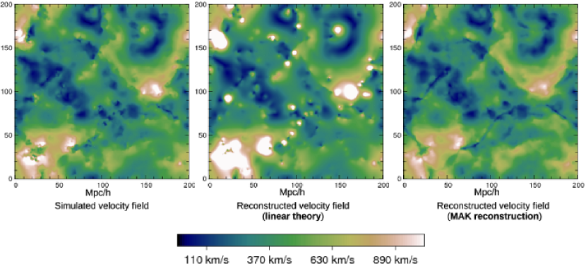
Figure 1: Illustration of the performance of reconstruction algorithms on a $N$-body simulation – Left panel: velocity field as given by the $N$-body simulation after evolution from Gaussian initial conditions. Middle panel: velocity field reconstructed using linear theory and the final dark matter distribution of the simulation. Right panel: velocity field reconstructed using the Monge-Ampère-Kantorovitch method and the final dark matter distribution of the simulation. The amplitude of the velocity field in a thin slice at the center of the simulation volume is represented in each panel. The scale is given by the bar below the panels.

While $N$-body sample gives an expected fair representation of the large scale dynamics, galaxy redshift catalog are unfortunately not that precise and complete due to intrinsic observational limitations. Lavaux et al. (2008) studied in details a lot of these limitations. We present in Table 1 a summary of the impact of these problems on the actual measurement of $\Omega_{\text{m}}$ obtained by looking at the relation between reconstructed and observed velocities. We note that we are essentially limited by the effect of the bias, which is our prior on the mass distribution according to the distribution of galaxies, for the determination of $\Omega_{\text{m}}$ from the velocity-velocity comparison. But, this does not increase scatter and the impact of the other effects seems under control.

Observational problem class	Effect	Observed systematic on $\Omega_{\text{m}}$
Mass distribution	Incompleteness	3-8%
	M/L assignment	20-46%
	Diffuse mass	50%
Redshift distortions	Finger-of-god	Small impact
	Kaiser effect	no large scale systematic
		potential small scale effect
Edge and finite volume effects	Zone of avoidance	No systematic, boundaries are affected
	Tidal effects	No systematic
	Cosmic variance	$\sim$20%
Statistical comparison	Velocity field correlation	Significant underestimation
		of error bar

Table 1: Observational effects on the measure of $\Omega_{\text{m}}$ from velocity-velocity comparison in redshift catalogs

2.5 The peculiar velocities in the Local Universe

As now we have assessed the importance of observational effects, we may reconstruct the peculiar velocities of our Local Universe. To achieve that goal, we used two catalogs: the Two-Micron All Sky Redshift Survey (2MRS) and the Nearby Galaxy 3,000 km.s^-1 (NBG-3k) distance catalog.

The 2MRS is based on the Two-Micron All Sky Survey (2MASS) photometric galaxy catalog. It is composed of about 25,000 galaxies, selected in the $K_{\text{S}}$ band with a magnitude limit of 11.25. Selecting according to $K_{\text{S}}$ allows us to have a fair sampling of the stellar mass in the 2MRS catalog by being sensitive mostly to the old population stars. It was then hoped to be a better indicator of the total galactic mass. Lin et al. (2004) and Ramella et al. (2004) showed that the luminosity in the K band is indeed a relatively good tracer of the mass with a mild dependence of the mass-to-light ratio to the luminosity. The other main advantage of the 2MRS is to be full sky and complete down to a galactic latitude of $b\sim 5-10$ degrees, depending whether we look in the direction of the galactic bulge. So, we are limited by the strong obscuration of galaxies in the direction of Milky Way’s galactic plane. The redshift galaxy distribution peaks at about $\sim 60-90$$h^{-1}$Mpc. This distribution is falling quickly above $\sim 120$$h^{-1}$Mpc, with only a handful of galaxies above $\sim 250$$h^{-1}$Mpc.

The NBG-3k is a 30-40$h^{-1}$Mpc deep galaxy catalog (Tully et al., 2008). It contains 1791 galaxies with high quality distances obtained from four different methods, when possible: the Tully-Fisher relation, the Tip of the red giant branch, the Surface Brightness fluctuation and the Fundamental plane.

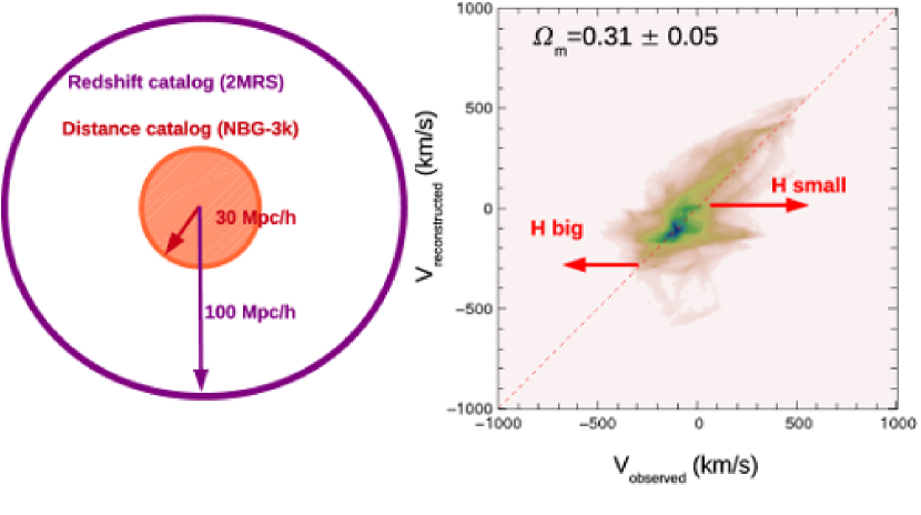
Figure 2: $\Omega_{\text{M}}$ estimation from peculiar velocities – Left panel: illustration giving the method of reconstruction and comparison. The reconstruction is achieved with a 100$h^{-1}$Mpc deep survey and the comparison is done on a 30$h^{-1}$Mpc deep volume where the two surveys overlap. Right panel: Scatter giving the relation between the reconstructed velocity against the observed velocity. The slope is relatively insensitive to the choice of the Hubble constant, which acts mostly by shifting the scatter along the horizontal axis. Here we assumed $H=83$ km.s^-1.Mpc^-1 and $\Omega_{\text{m}}=0.31$ for representing the scatter.

Using the 2MRS, we run a 100$h^{-1}$Mpc deep reconstruction for a comparison with observed velocities in a 30$h^{-1}$Mpc deep volume. This is sufficiently big to mitigate boundary effects in the volume of comparison, while not too big to be strongly affected by shot noise effects due to poorer mass sampling above 60$h^{-1}$Mpc. More details on this reconstruction are given in Lavaux et al. (2008).

In Fig. 2, we represented the result of the comparison between reconstructed and observed velocities in the 30$h^{-1}$Mpc deep volume. We estimated $\Omega_{\text{m}}=0.31\pm 0.05$ using the slope of the scatter plot (Lavaux et al., 2008). This slope is independent of any arbitrary calibration problem in the Hubble constant we determined from data. The Hubble constant would move the scatter along the horizontal axis but would not change the slope.

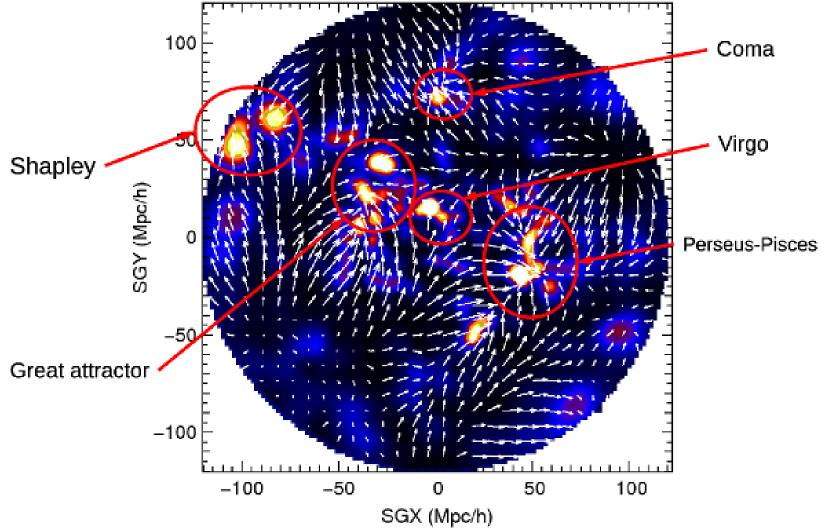
Figure 3: Reconstructed velocity field in the Supergalactic plane – We represent the reconstructed velocity field in an infinitesimally thin slice around the Supergalactic plane $SGZ=0$. We highlight the major structure present in this plane. Here, we use a 120$h^{-1}$Mpc deep cut of the 2MASS Redshift Survey for reconstructing the peculiar velocity field.

In Fig. 3, we represented the reconstructed velocity field in an infinitesimally thin cut around the Supergalactic plane. We highlight the known large structures of the Local Universe with red circles along with their names. It happens that all these major structures lie on this plane. We also note the presence of large flows falling towards this structures as expected. At the same time, there is no divergence of these flows in the immediate neighborhood, highlighting the quality of the MAK reconstruction.

Now, we also note the presence of a relatively large void in the lower-left part of the panel. From this region the matter seems to escape. This pushes the idea that we not only study clusters of galaxies but also voids using the peculiar velocities.

3 Studying void dynamics

In the previous section, we described a way to study peculiar velocity dynamic using the MAK reconstruction method. We are now presenting how this technique can be transported to the study of voids in large and deep galaxy surveys.

3.1 Identifying voids in large-scale structures

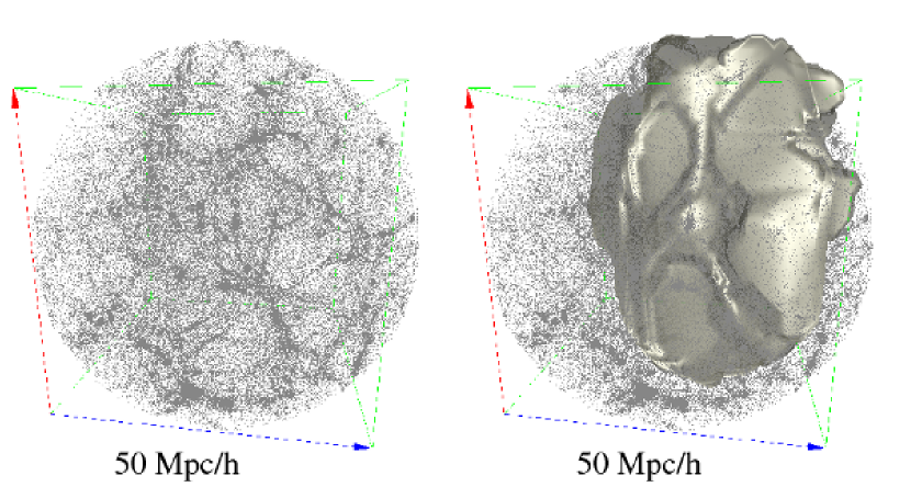
Figure 4: Voids in large-scale structures – Right panel: An example of a void found and whose volume has been determined in Lagrangian coordinates and transported to Eulerian coordinates (4$h^{-1}$Mpc smoothing scale in Lagrangian coordinates). The dots correspond to the actual position of the particles of the simulation. We see that the highlighted boundary follows the distribution. The scale of the box is 50$h^{-1}$Mpc.

Voids are large strongly underdense region of the Universe, that we know most probably forms by gravitational instabilities from primordial density fluctuations (Hoffman and Shaham, 1982; Hoffman et al., 1983; Hausman et al., 1983). One of these voids is illustrated in the particle distribution given by a $N$-body simulation in the left panel of Fig. 4.

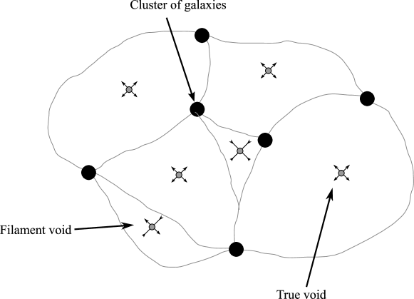
Figure 5: We give an illustration of the dynamical scheme we propose to study voids and why it is important. Actual observed voids may be contracting (represented by the arrows pointing towards the center of void) or expanding (arrows going away from center). Contracting voids are not distinguished from expanding voids with standard Eulerian void finder techniques.

Since their discovery by Gregory and Thompson (1978); Tully and Fisher (1978); Kirshner et al. (1981) in galaxy redshift surveys, a lot of work has gone into finding a reliable way of detecting and characterizing the voids in large galaxy catalogs. We can separate all these void finders in three broad classes: galaxy based void finders, for which we look for holes in a distribution of galaxies, density based void finders, for which we try to find geometrical patterns in the total matter density field inferred from galaxy distribution, and dynamical void finders, for which gravitationally unstable points are derived from this same distribution.

Even though the number of void finders was flourishing, the large physical size of the voids has for a long time hindered their use as a probe for fundamental cosmological physics. With nowadays deep photometric and spectroscopic surveys of galaxies, this starts being possible to accumulate sufficient statistics. However, we still miss a simple and usable definition of a void that would allow us to compute statistical properties of these objects. Their potential of information is important as they represent the counterpart of the cluster: we can count them, describe their shape and their size, just as for clusters, which already yields important constraints on cosmological parameters (e.g. Vikhlinin et al., 2009, for the latest attempt)

We propose a new definition and a new technique for identifying voids in the matter density field, which is described in more details in Lavaux and Wandelt (2009). This technique is built upon the success of the Monge-Ampère-Kantorovitch reconstruction. We identify voids with the main source of displacement field, such as illustrated in Fig. 5, which is properly reconstructed by the MAK method, after smoothing in Lagrangian coordinates. This smoothing step means that we probe structures in a particular dynamical collapse time. As voids are in different collapse time, it is necessary to smooth at different scales to probe all possible void statistics. Here, we will present the results only for one smoothing scale. We choose the center of the voids to correspond with the maximum of the divergence of the displacement field, which is then considered to be sourced by the voids. The geometry of the voids themselves may be determined subsequently by considering a watershed (Platen et al., 2007) transform of the divergence of the displacement field. The boundaries are then transported using the displacement field to their proper Eulerian position. An illustration of a void found using this technique is given in the right panel of Fig. 4.

Using the first derivatives of the displacement at the position of the center of the voids, we define the ellipticity, as in Park and Lee (2007):

$$\varepsilon=1-\sqrt{\frac{1+\lambda_{3}}{1+\lambda_{1}}}$$ (5)

with $\lambda_{1}>\lambda_{2}>\lambda_{3}$ the eigenvalues of the Jacobian matrix of the displacement field. This ellipticity measures the amount of local shear of the matter density field at the center of the voids. On one hand, this ellipticity is linked to the overall ellipticity of the volume, although in a non-trivial manner. On the other hand, being linked to a reasonably linear quantity as the displacement field, the tidal ellipticity may be properly modelled analytically and at same time measured in simulation and observational data.

3.2 Measuring Dark Energy properties

We modeled the ellipticity statistics using Zel’dovich approximation and Gaussian random field statistics in Lavaux and Wandelt (2009). Compared to the work by Park and Lee (2007), we introduced correlations on the density/gravity curvature, as we essentially identify voids with the proto-voids in the primordial density field.

In the left panel of Fig. 6, we show that the comparison between analytic modeling (colored solid curves) and ellipticity measured in simulation is impressive for our model.

In the right panel of Fig. 6, we compare the evolution of the mean ellipticity in two $w$CDM cosmologies, $w=-1$ and $w=-0.5$. The residual between the model and the actual measurements in the simulation are shown in the bottom part of the panel. The residual in not bigger than $\sim 1\%$ and most of it comes from the actual variance of the initial condition of the simulation. This effect will not prevent applying this method to observations for two reasons. First, we will marginalize over the bias and so the systematic shift will disappear. Second, each considered slice should be a nearly independent random realization of a Gaussian random field normalized to the same $\sigma_{8}$. Thus the points should be scattered according to our dashed horizontal line “0%” and not systematically pushed up or down. We see that the points fall right onto the curves given by the two models. This shows that this method is a very promising tool to investigate dark energy physical property like its equation of state $w$.

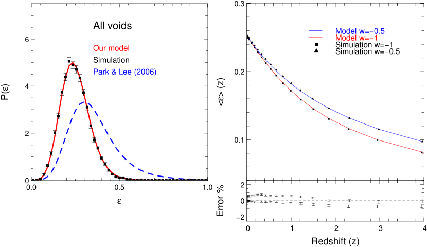
Figure 6: Ellipticity statistic modeling – Left panel: Comparison between the measured ellipticity distribution in simulation and the prediction given by our model and the original statistical model of Park and Lee (2007). The difference comes from the introduction of the correlation between density and gravity. Error bars on the points coming from simulation are estimated by assuming Poisson distribution on the binned values. Right panel: Evolution of the mean ellipticity with redshift for the two $w$CDM cosmology with the residual between the actual measured points in the simulation and the model. The error bars on the residual are estimated from the intrinsic error in estimating the ellipticity and the number of averaged points.

4 Conclusion

In this paper, we have considered one particular method of reconstruction of peculiar velocities and applied it both to simulation and observation. Its performance at reconstructing simulated velocity field is impressive and far better than linear theory. This performance is now limited by our assumptions on the distribution of dark matter (the galaxy bias problem).

We have applied our method with success on the Two-Micron-All-Sky redshift survey. The comparison between observed and reconstructed peculiar velocities is good and yielded an $\Omega_{\text{m}}$ in agreement with the value given by other cosmological probes, such as WMAP results (Dunkley et al., 2008). In the future, we will aim at improving the statistics of the comparison.

It is possible to use reconstructed peculiar velocities for another related study: the identification of voids in galaxy surveys and their use for probing cosmological parameters such as the Dark Energy equation of state. As the displacement field, and the related peculiar velocity field, is still essentially linear, it is possible to make a simple model linking the local shape of voids, which is the ellipticity $\varepsilon$, to the background cosmology. We achieved this comparison with total success in $N$-body simulation. We will aim at using this method in real galaxy survey, like the Sloan Digital Sky Survey, to improve the constraints on $w$.

References

- Watkins et al. (2009) R. Watkins, H. A. Feldman, and M. J. Hudson, MNRAS 392, 743–756 (2009), 0809.4041.
- Haynes et al. (1999) M. P. Haynes, R. Giovanelli, P. Chamaraux, L. N. da Costa, W. Freudling, J. J. Salzer, and G. Wegner, AJ 117, 2039–2051 (1999).
- Wegner et al. (1999) G. Wegner, M. Colless, R. P. Saglia, R. K. McMahan, R. L. Davies, D. Burstein, and G. Baggley, MNRAS 305, 259–296 (1999), arXiv:astro-ph/9811241.
- Springob et al. (2007) C. M. Springob, K. L. Masters, M. P. Haynes, R. Giovanelli, and C. Marinoni, ApJS 172, 599–614 (2007).
- Masters et al. (2008) K. L. Masters, C. M. Springob, and J. P. Huchra, AJ 135, 1738–1748 (2008), 0711.4305.
- Herrnstein et al. (1999) J. R. Herrnstein, J. M. Moran, L. J. Greenhill, P. J. Diamond, M. Inoue, N. Nakai, M. Miyoshi, C. Henkel, and A. Riess, Nature 400, 539–541 (1999), arXiv:astro-ph/9907013.
- Karachentsev et al. (2003) I. D. Karachentsev, D. I. Makarov, M. E. Sharina, A. E. Dolphin, E. K. Grebel, D. Geisler, P. Guhathakurta, P. W. Hodge, V. E. Karachentseva, A. Sarajedini, and P. Seitzer, Astron. Astrophys. 398, 479–491 (2003), URL http://arxiv.org/abs/astro-ph/0211011, astro-ph/0211011.
- Lee et al. (1993) M. G. Lee, W. L. Freedman, and B. F. Madore, Astrophys. J. 417, 553+ (1993), URL http://dx.doi.org/10.1086\%2F173334.
- Tonry and Schneider (1988) J. Tonry, and D. P. Schneider, Astron. J. 96, 807–815 (1988), URL http://dx.doi.org/10.1086\%2F114847.
- Tonry et al. (2001) J. L. Tonry, A. Dressler, J. P. Blakeslee, E. A. Ajhar, A. B. Fletcher, G. A. Luppino, M. R. Metzger, and C. B. Moore, Astrophys. J. 546, 681–693 (2001), URL http://arxiv.org/abs/astro-ph/0011223, astro-ph/0011223.
- Tully and Fisher (1977) R. B. Tully, and J. R. Fisher, A&A 54, 661–673 (1977).
- Faber and Jackson (1976) S. M. Faber, and R. E. Jackson, ApJ 204, 668–683 (1976).
- Peebles (1976) P. J. E. Peebles, ApJ 205, 318–328 (1976).
- Brenier et al. (2003) Y. Brenier, U. Frisch, M. Hénon, G. Loeper, S. Matarrese, R. Mohayaee, and A. Sobolevskiĭ, MNRAS 346, 501–524 (2003), astro-ph/0304214.
- Lavaux et al. (2008) Lavaux, G., Mohayaee, R., Colombi, S., Tully, R. B., Bernardeau, F., Silk, and J., Monthly Notices of the Royal Astronomical Society 383, 1292–1318 (2008), ISSN 0035-8711, URL http://arxiv.org/abs/0707.3483, 0707.3483.
- Bertsekas (1979) D. P. Bertsekas, A Distributed Algorithm for the Assignment Problem, MIT Press, Cambridge, MA, 1979.
- Bertsekas (1998) D. Bertsekas, Network Optimization: Continuous and Discrete Models, Athena Scientific, 1998.
- Lin et al. (2004) Y. Lin, J. J. Mohr, and S. A. Stanford, ApJ 610, 745–761 (2004), arXiv:astro-ph/0402308.
- Ramella et al. (2004) M. Ramella, W. Boschin, M. J. Geller, A. Mahdavi, and K. Rines, AJ 128, 2022–2036 (2004), arXiv:astro-ph/0407640.
- Tully et al. (2008) R. B. Tully, E. J. Shaya, I. D. Karachentsev, H. Courtois, D. D. Kocevski, L. Rizzi, and A. Peel, Astrophys. J. 676, 184–205 (2008), URL http://arxiv.org/abs/0705.4139, 0705.4139.
- Lavaux et al. (2008) G. Lavaux, R. B. Tully, R. Mohayaee, and S. Colombi, ArXiv e-prints (2008), 0810.3658.
- Hoffman and Shaham (1982) Y. Hoffman, and J. Shaham, ApJL 262, L23–L26 (1982).
- Hoffman et al. (1983) G. L. Hoffman, E. E. Salpeter, and I. Wasserman, ApJ 268, 527–539 (1983).
- Hausman et al. (1983) M. A. Hausman, D. W. Olson, and B. D. Roth, ApJ 270, 351–359 (1983).
- Gregory and Thompson (1978) S. A. Gregory, and L. A. Thompson, ApJ 222, 784–799 (1978).
- Tully and Fisher (1978) R. B. Tully, and J. R. Fisher, “Nearby small groups of galaxies,” in Large Scale Structures in the Universe, edited by M. S. Longair, and J. Einasto, 1978, vol. 79 of IAU Symposium, pp. 31–45.
- Kirshner et al. (1981) R. P. Kirshner, A. Oemler, Jr., P. L. Schechter, and S. A. Shectman, ApJL 248, L57–L60 (1981).
- Vikhlinin et al. (2009) A. Vikhlinin, A. V. Kravtsov, R. A. Burenin, H. Ebeling, W. R. Forman, A. Hornstrup, C. Jones, S. S. Murray, D. Nagai, H. Quintana, and A. Voevodkin, ApJ 692, 1060–1074 (2009), 0812.2720.
- Lavaux and Wandelt (2009) G. Lavaux, and B. D. Wandelt, ArXiv e-prints (2009), 0906.4101.
- Platen et al. (2007) E. Platen, R. van de Weygaert, and B. J. T. Jones, MNRAS 380, 551–570 (2007), 0706.2788.
- Park and Lee (2007) D. Park, and J. Lee, Physical Review Letters 98, 081301–+ (2007).
- Dunkley et al. (2008) J. Dunkley, E. Komatsu, M. R. Nolta, D. N. Spergel, D. Larson, G. Hinshaw, L. Page, C. L. Bennett, B. Gold, N. Jarosik, J. L. Weiland, M. Halpern, R. S. Hill, A. Kogut, M. Limon, S. S. Meyer, G. S. Tucker, E. Wollack, and E. L. Wright, ArXiv e-prints 803 (2008), URL http://arxiv.org/abs/0803.0586, 0803.0586.