Transient response under ultrafast interband excitation of an intrinsic graphene

Abstract

The transient evolution of carriers in an intrinsic graphene under ultrafast excitation, which is caused by the collisionless interband transitions, is studied theoretically. The energy relaxation due to the quasielastic acoustic phonon scattering and the interband generation-recombination transitions due to thermal radiation are analyzed. The distributions of carriers are obtained for the limiting cases when carrier-carrier scattering is negligible and when the intercarrier scattering imposes the quasiequilibrium distribution. The transient optical response (differential reflectivity and transmissivity) on a probe radiation and transient photoconductivity (response on a weak dc field) appears to be strongly dependent on the relaxation and recombination dynamics of carriers.

I Introduction

The transient response of photoexcited carriers under ultrafast interband pumping has been studied during the last decades in bulk semiconductors and heterostructures (see Ref. 1 for review). The unusual transport of carriers in graphene is caused by a neutrinolike energy spectrum in gapless semiconductor, which is described by the Weyl-Wallace model 2 , and a substantial modification of scattering processes. Recently, the properties of graphene after ultrafast interband excitation attract special attention. The experimental results in relaxation dynamics of photoexcited electrons and holes were published in 3 ; 4 ; 5 and 6 for epitaxial and exfoliated graphene, respectively. The relaxation of nonequilibrium optical phonons, which are emitted by carriers after photoexcitation, is studied in Ref. 7. The theoretical consideration of the carrier relaxation and generation-recombination processes caused by optical phonons is performed in 8 ; 9 . The quasielastic energy relaxation of carriers due to acoustic phonons was considered in 10 ; 11 for low energy carriers (at low temperatures or under mid-IR excitation). In particular, an interplay between energy relaxation and generation-recombination processes determines the relaxation dynamics of photoexcited carrier distribution. 10 To the best of our knowledge, both this interplay and the relaxation dynamics at low temperatures are not considered so far. Thus, the investigation of the transient response of carriers under these conditions is timely now.

In this paper, we consider the transient response of an intrinsic graphene in case of ultrafast interband excitation in passive region, where the carrier energies are smaller than the optical phonon energy. Such a regime can be realized under the pumping in the mid-infrared (IR) spectral region or at low temperatures, when the peak of photoexcited carriers formed after the process of optical phonon emission, remains a narrow one. Describing the photoexcitation process, we restrict ourselves by the collisionless regime, when a pulse duration, $\tau_{p}$, is shorter than the momentum relaxation time. Considering the low-temperature transient dynamics of photoexcited carriers, one takes into account the intraband quasielastic energy relaxation due to acoustic phonons and generation-recombination interband transitions due to thermal radiation. The carrier-carrier scattering is described within two limiting regimes: ($i$) when the Coulomb interaction is unessential, and ($ii$) when intercarrier scattering imposes the quasiequilibrium distribution of carriers. With the obtained transient distribution of carriers, we analyze a time-dependent response on the probe field, i.e. we consider the transient reflection and transmission in THz and mid-IR spectral regions. The transient photoconductivity is also analyzed below, because the energy relaxation corresponds to a nanosecond scale (the radiative recombination remains essential up to microsecond).

Since the electron-hole energy spectrum and scattering processes are symmetric in an intrinsic graphene, the phenomena under consideration are described by the same distribution functions for electrons and holes, $f_{pt}$. Such distribution is governed by the general kinetic equation 12 :

$$\frac{\partial f_{pt}}{\partial t}=\sum_{k}J_{k}\left\{f_{t}|p\right\}+G\{f|pt\},$$ (1)

where the collision integrals $J_{k}\left\{f_{t}|p\right\}$ describe the relaxation of carriers caused by the carrier-carrier scattering ($k=cc$), the acoustic phonons ($k=ac$), and the thermal radiation ($k=r$), respectively. The photogeneration rate, $G\{f|pt\}$, describes the interband excitation of electron-hole pairs by the mid-IR ultrafast pulse. Below Eq. (1) is solved with the initial condition $f_{pt\to-\infty}=f_{p}^{(eq)}$, where $f_{p}^{(eq)}$ is the equilibrium distribution. The transient response on a probe radiation is described by the dynamic conductivity due to interband transitions. The transient response on a weak dc field (photoconductivity) is considered with the use of the phenomenological model of momentum scattering suggested in 13 .

The analysis carried out below is organized as follows. The photoexcitation process under the inerband pumping is described in Sec. II. The transient evolution distributions are given in Sec. III for the cases ($i$) and ($ii$). Section IV presents a set of results of transient reflectivity and transmittivity, and also the transient photoconductivity. The discussion of the assumptions used and concluding remarks are given in the last section. Appendix contains the microscopical evaluation of the interband photogeneration rate under ultrafast interband excitation.

II Ultrafast excitation

In the framework of the Weyl-Wallace model (spin- and valley-degenerate linear energy spectrum of carriers which is determined by the characteristic velocity $v_{W}$), the interband photoexcitation is caused by the in-plane electric field, $w_{t}{\bf E}\exp(-i\Omega t)+c.c.$ where $\bf E$ is the field strength, $\omega$ is the frequency, and $w_{t}$ is the envelope form-factor. Eq. (1) is transformed to the collisionless form on the initial intervals, when scattering mechanisms are not essential: $\partial f_{pt}/\partial t=G\left\{{f|pt}\right\}$. Using the boundary condition of Eq. (1), one can rewrite this equation in the integral form $f_{pt}=f_{p}^{(eq)}+\int_{-\infty}^{t}dt^{\prime}G\{f|pt^{\prime}\}$. The photogeneration rate here is evaluated in Appendix as follows:

$$G\left\{f|pt\right\}=\left(\frac{eEv_{W}}{\hbar\Omega}\right)^{2}w_{t}\int\limits_{-\infty}^{0}d\tau w_{t+\tau}$$

$$\times\cos\left[\left(\frac{2v_{W}p}{\hbar}-\Omega\right)\tau\right]\left(1-2f_{pt+\tau}\right),$$ (2)

where the Pauli blocking factor $(1-2f_{pt+\tau})$ is responsible for the coherent Rabi oscillations of the excited carriers.

Introducing the dimensionless intensity, $I_{ex}=(eE\tau_{p}v_{W}/\hbar\Omega)^{2}$, we consider below the linear regime of excitation which takes place if $I_{ex}\ll 1$ and $f_{pt}\ll 1$, so that the Pauli factor can be neglected (if $\hbar\Omega$ comparable to the equilibrium temperature $T$ one has to use the equilibrium Pauli factor in Eq. (2)). Using the Gaussian form-factor $w_{t}=\sqrt[4]{2/\pi}\exp\left[-\left(t/\tau_{p}\right)^{2}\right]$ with the pulse duration $\tau_{p}$, 14 one obtaines the photoexcited distribution in the form

$$f_{pt}^{(ex)}\approx I_{ex}\int\limits_{-\infty}^{t}{dt^{\prime}}w_{t^{\prime}}\int\limits_{-\infty}^{0}{d\tau w_{t^{\prime}+\tau}\cos\left({\frac{{2v_{W}\delta p}}{\hbar}\tau}\right)}.$$ (3)

Here $\delta p=p-p_{\Omega}$ is centred in the characteristic momentum $p_{\Omega}=\hbar\Omega/2v_{W}$. The evolution of photoexcited distribution, $f_{pt}^{(ex)}/I_{ex}$, is shown in Fig. 1. The distribution is dependent on $t/\tau_{p}$ and $\delta p/\Delta p$, where $\Delta p=\hbar/2v_{W}\tau_{p}$ determines the width of distribution which is proportional to $\tau_{p}^{-1}$. For $t\gg\tau_{p}$, the integrations in Eq. (3) can be exactly performed and we obtain steady-state distribution after the photoexcitation pulse, $f_{p}^{(ex)}=f_{pt\to\infty}^{(ex)}$, as the Gaussian peak of width $\propto\Delta p$:

$$f_{p}^{(ex)}=\sqrt{\frac{\pi}{2}}I_{ex}e^{-(\delta p/\sqrt{2}\Delta p)^{2}}.$$ (4)

Thus, at $t\geq 2\tau_{p}$ (see Fig. 1) one can omit the photogeneration rate in Eq. (1) using instead the initial condition:

$$f_{pt=0}=f_{p}^{(eq)}+f_{p}^{(ex)},$$ (5)

which is given as a sum of the equilibrium and photoexcited contributions. The condition (5) can be used directly in case of weak intercarrier scattering. In case of optical excitation, with a subsequent emission of cascade of $2{\cal N}$ optical phonons of energy $\hbar\omega_{0}$, the photoexcited distribution can be written in the form (5) where $\delta p$ is centred in $p_{\overline{\omega}}=(\hbar\Omega-2{\cal N}\hbar\omega_{0})/2v_{W}$ and $\Delta p$ is included an additional broadening during the cascade emission.

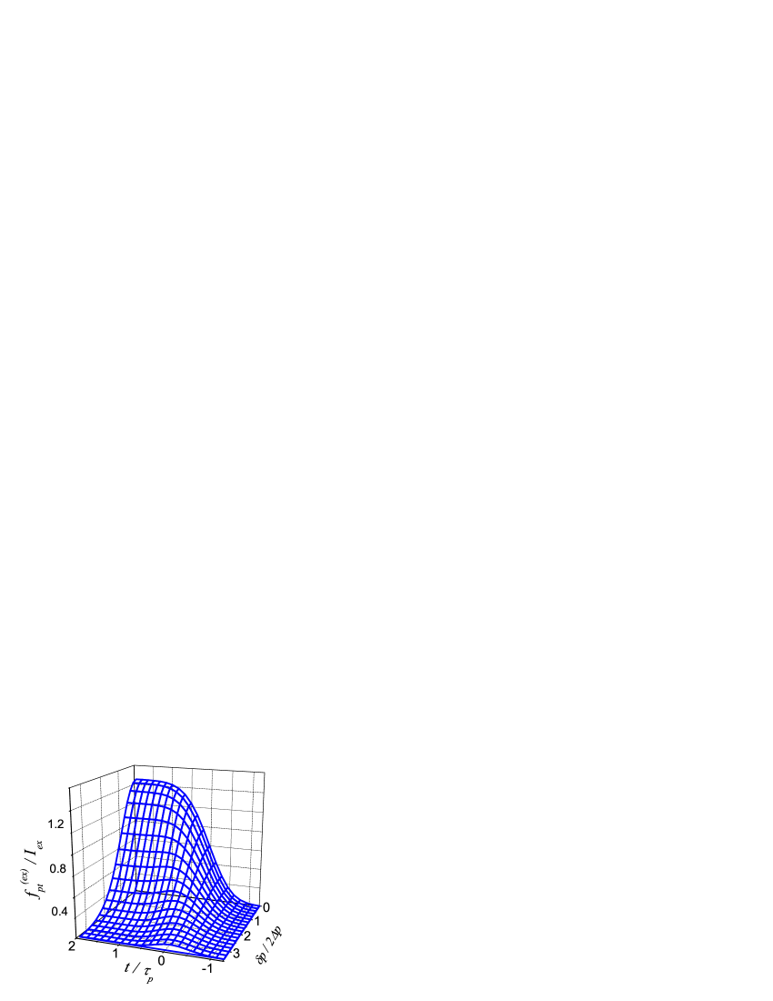
Figure 1: Temporal evolution of photoexcited distribution $f_{pt}^{(ex)}$ normalized to $I_{ex}$ versus dimensionless momentum and time, $\delta p/2\Delta p$ and $t/\tau_{p}$.

Under an effective intercarrier scattering, one needs to calculate the initial temperature and concentration of carriers. The photoexcited concentration and energy of carriers, which are described by the peak of distribution (4) are given by

$$\left|\begin{array}[]{*{20}c}\Delta n_{ex}\\ \Delta E_{ex}\end{array}\right|=\frac{4}{L^{2}}\sum\limits_{\bf p}\left|\begin{array}[]{*{20}c}1\\ {v_{W}p}\end{array}\right|f_{p}^{(ex)}\simeq\frac{I_{ex}(\overline{\omega}/v_{W})^{2}}{2\overline{\omega}\tau_{p}}\left|\begin{array}[]{*{20}c}1\\ \hbar\overline{\omega}/2\end{array}\right|,$$ (6)

where $L^{2}$ is the normalization area. One obtains $\Delta E_{ex}/n_{ex}=\hbar\overline{\omega}/2$, for the Gaussian shape of pulse, i.e. the averaged energy per generated particle is equal to the excitation energy. In case of optical excitation, with $\cal N$ optical phonons emitted, the energy per photoexcited particle, $\Delta E_{ex}/\Delta n_{ex}$, agrees closely with $\hbar\omega-{\cal N}\hbar\omega_{0}$ (see above).

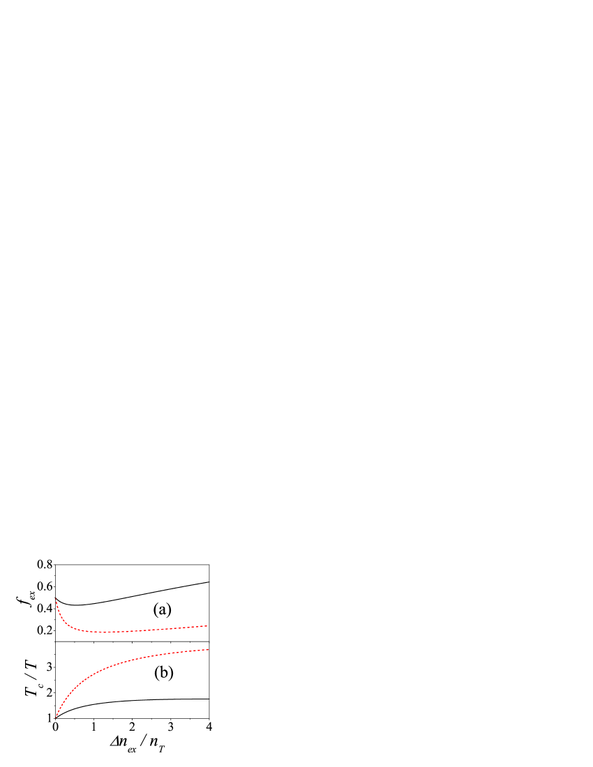
Figure 2: Initial maximum distribution (a) and effective temperature (b), $f_{ex}$ and $T_{ex}$, versus pumping ($\Delta n_{ex}/n_{T}\propto I_{ex}$ for $\hbar\overline{\omega}=60$ meV and 120 meV (solid and dashed curves, respectively).

If $\tau_{p}\ll\tau_{cc}\ll\tau_{ac,r}$ , where $\tau_{cc}$, $\tau_{ac}$, and $\tau_{r}$ correspond to the intercarrier scattering, the energy relaxation, and the generation-recombination processes, respectively [the Coulomb-controlled case ($ii$)], the dominanting carrier-carrier scattering imposes the quasi-equilibrium distribution

$$f_{pt}=\left[\exp\left(\frac{v_{W}p-\mu_{t}}{T_{t}}\right)+1\right]^{-1}$$ (7)

with the effective temperature $T_{t}$ and the quasichemical potential $\mu_{t}$. If $\tau_{cc}\ll t\ll\tau_{ac,r}$, the initial values $T_{ex}=T_{t\to 0}$ and $f_{ex}=f_{p=0t\to 0}$ are determined from the concentration and energy conservation requirements:

$$\frac{2}{\pi}\left(\frac{T_{ex}}{\hbar v_{W}}\right)^{2}\int\limits_{0}^{\infty}dxxf_{x}\left|{\begin{array}[]{*{20}c}1\\ {T_{ex}x}\\ \end{array}}\right|=\left|{\begin{array}[]{*{20}c}{n_{T}+\Delta n_{ex}}\\ {E_{T}+\Delta E_{ex}}\\ \end{array}}\right|,$$ (8)

where the function $f_{x}$ is introduced according to $f_{x}\equiv f_{ex}/[e^{x}(1-f_{ex})+f_{ex}]$. Using $\Delta n_{ex}$ and $\Delta E_{ex}$ given by Eq. (6) and solving the transcendental system (8) one obtains the initial values $f_{ex}$ and $T_{ex}$. The calculations here and below are performed for the nitrogen temperature, $T=$77 K, the excitation energies $2v_{W}p_{\overline{\omega}}=$120 meV (CO₂ laser) and 60 meV (as an example of interband excitation with subsequent optical phonon emission), and the broadening energy $\hbar/\tau_{p}\simeq$6.6 meV, which corresponds to the pulse duration $\simeq$0.1 ps. In Fig. 2 we plot $f_{ex}$ and $T_{ex}$ versus the pumping level which is proportional to $\Delta n_{ex}/n_{T}$. Fast increase of $T_{ex}$ and fast decrease of $f_{ex}$ take place for $\Delta n_{ex}/n_{T}<1$, while a linear increase of these values are realized if $\Delta n_{ex}/n_{T}>1$.

III Energy relaxation and recombination

In this section we analyze the transient evolution of $f_{pt}$ caused by the energy relaxation and recombination processes. We consider the cases ($i$) and ($ii$), when the initial condition is given by Eq. (5) and written through $f_{ex}$ and $T_{ex}$ plotted in Fig. 2.

III.1 Weak intercarrier scattering

If the carrier-carrier scattering is ineffective [case ($i$)], the distribution $f_{pt}$ is governed by the kinetic equation (1) without the $cc$-contribution

$$\frac{\partial f_{pt}}{\partial t}=\frac{\nu_{p}^{\ss(qe)}}{p^{2}}\frac{d}{dp}\left\{p^{4}\left[\frac{df_{pt}}{dp}+\frac{f_{pt}(1-f_{pt})}{p_{T}}\right]\right\}$$

$$+\nu_{p}^{(r)}[N_{2p/p_{T}}(1-2f_{pt})-f_{pt}^{2}]$$ (9)

and with the initial condition (5) used instead of generation rate. Here we substituted the explicit expressions of the collision integrals for the quasielastic acoustic scattering approximation (written in the Fokker-Planck form) and for the generation-recombination processes, see discussion in 10 . The Planck distribution $N_{2p/p_{T}}$ is written through $p_{T}=T/v_{W}$ while the energy relaxation rate $\nu_{p}^{(qe)}=v_{qe}p/\hbar$ and the rate of radiative transitions $\nu_{p}^{(r)}=v_{r}p/\hbar$ are written through the characteristic velocities $v_{qe}\propto T$ and $v_{r}$ 15 .

The boundary conditions are imposed by both the condition $f_{p\to\infty t}=0$, which is transformed into the requirement

$$p^{4}\left(\frac{\partial f_{pt}}{\partial p}+\frac{f_{pt}}{p_{T}}\right)_{p\to\infty}<{\rm const},$$ (10)

and Eq. (9) at $p=0$ which is transformed into the initial condition $f_{p=0t}=1/2+f_{p=0}^{(ex)}\exp[-(v_{r}/v_{W})Tt/\hbar]$. According to Eq. (4) one obtains $f_{p=0}^{(ex)}=\sqrt{\pi/2}I_{ex}\exp[-(\Omega\tau_{p})^{2}/2]\ll 1$ and one can neglect the second contribution in this initial condition, so that $f_{p=0t}=1/2$. Numerical solution of the Cauchy problem given by Eqs. (5), (9), and (10) is obtained below by the use of the iteration procedure. 16

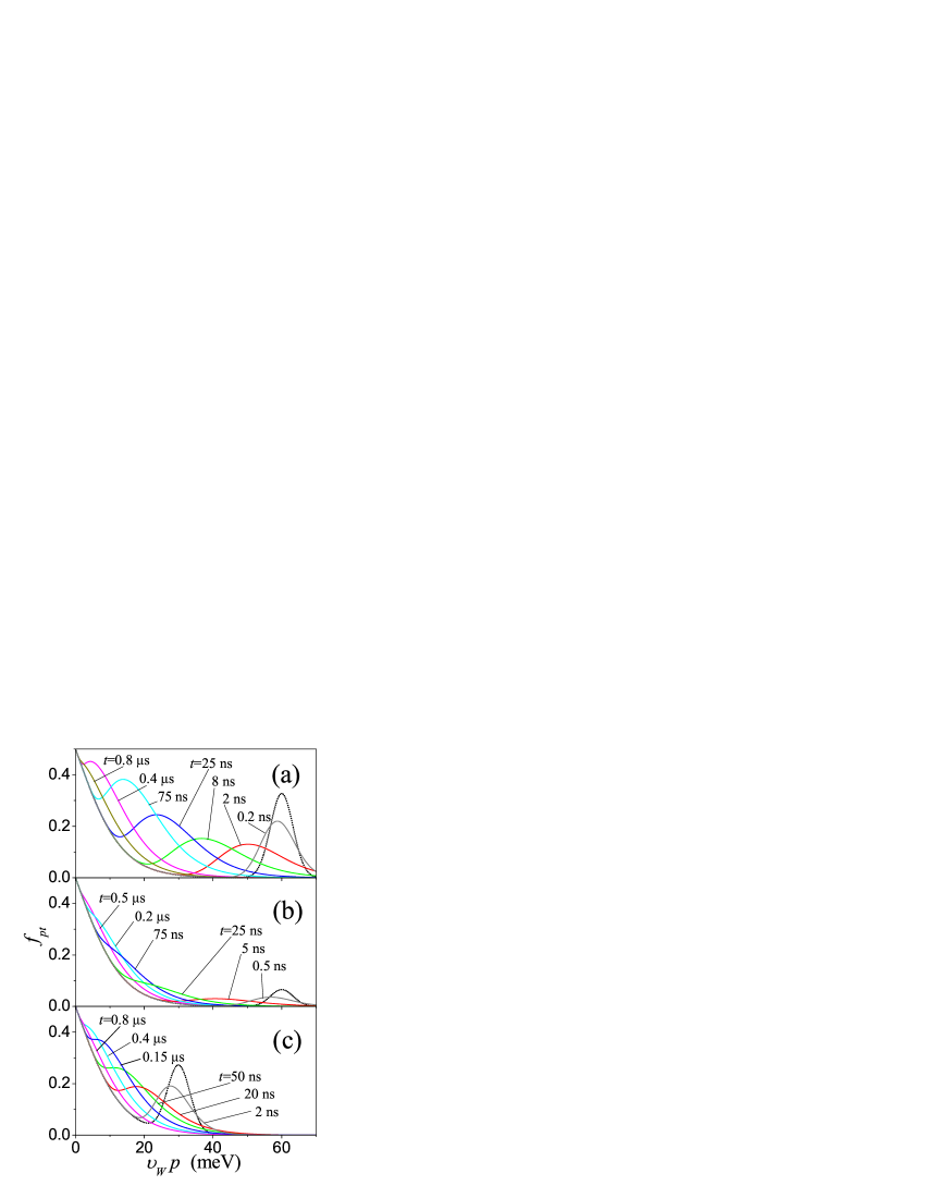
Figure 3: Distribution $f_{pt}$ versus carrier energy $pv_{W}$ for different delay times (marked) and excitation conditions: (a) $\hbar\overline{\omega}=$120 meV and $I_{ex}=$0.26, (b) $\hbar\overline{\omega}=$120 meV and $I_{ex}=$0.05, and (c) $\hbar\overline{\omega}=$60 meV and $I_{ex}=$0.21.

In Fig.3 we demonstrate the evolution of the distribution $f_{pt}$ at 77 K for the cases when carriers are excited around the energies 60 meV and 30 meV. The delay times are marked in panels a-c and the pumping levels are determined through the initial peak value, given by $\sqrt{\pi/2}I_{ex}$, see Eq. (4)). Under mid-IR pumping with pulse duration $\tau_{p}=$0.1 ps and the spot sizes $\sim$0.5 mm the above-used pumping levels correspond to the pulse energies $\sim$85 pJ and $\sim$17 pJ for Figs. 3a and 3b, respectively, see 17 for experimental details. Under optical pumping ($\hbar\Omega\sim$1.6 eV) and subsequent emission of phonon cascade, the pumping level in Fig. 3c corresponds to the pulse energy $\sim$12 nJ (duration and size are the same as above). One can see that the transient evolution of distribution occurs in two stages: energy relaxation and recombination. During the first stage (about $t\lesssim$50 ns, which is dependent on position and maximum value $f_{p}^{(ex)}$; compare with Figs. 3a-c) the initial peak is tranformed into the quasiequilibrium high-energy tail (with the equilibrium temperature caused by the energy relaxation) which is connected to the low-energy equilibrium distrbution. During the next stage (up to 1 $\mu$s) the high-energy tail shifts to the lower energies and transforms into the equilibrium distribution due to effective radiative recombination in low-energy region.

III.2 Coulomb-controlled case

In the carrier-carrier scattering case ($ii$), one has to describe the transient evolution of the effective temperature $T_{t}$ and the maximum distribution $f_{t}=f_{p=0t}$, that replaces the chemical potential. Since the intercarrier scattering change neither the concentration, $n_{t}=(4/L^{2})\sum_{\bf p}f_{pt}$, nor the energy of carriers, $E_{t}=(4/L^{2})\sum_{\bf p}v_{W}pf_{pt}$, the balance equations for $n_{t}$ and $E_{t}$ take forms: 18

$$\frac{d}{{dt}}\left|{\begin{array}[]{*{20}c}{n_{t}}\\ {E_{t}}\\ \end{array}}\right|=\frac{4}{{L^{2}}}\sum\limits_{\bf p}{\left|{\begin{array}[]{*{20}c}{J_{r}\{f_{t}|p\}}\\ {v_{W}p\left[{J_{ac}\{f_{t}|p\}+J_{r}\{f_{t}|p\}}\right]}\\ \end{array}}\right|}.$$ (11)

Further, we transform the balance equations, expressing the left-hand side of (11) through $T_{t}$ and $f_{t}$ as follows:

$$\frac{d}{dt}\left(T_{t}^{2}A_{t}^{(1)}\right)=R_{t}^{(1)},$$ (12)

$$\frac{d}{dt}\left(T_{t}^{3}A_{t}^{(2)}\right)=R_{t}^{(2)}+Q_{t}.$$

Here the coefficients $A_{t}^{(1,2)}$ are written as $A_{t}^{(q)}=\int_{0}^{\infty}dxx^{q}f_{xt}$, where the quasiequilibrium distribution is given by $f_{xt}=f_{t}/\left[e^{x}(1-f_{t})+f_{t}\right]$, so that $A_{t}^{(q)}/T_{t}^{l}$ are only depend on $f_{t}$. After substitution of the collision integrals $J_{r}$ 10 ; 18 and integration, the generation-recombination contributions to Eq. (12) are obtained in the form

$$R_{t}^{(q)}=\frac{2v_{r}T_{t}^{q+2}}{v_{W}\hbar}\int\limits_{0}^{\infty}dxx^{q+2}f_{xt}^{2}\left[\frac{e^{2x}(1-f_{t})^{2}}{(e^{x2T_{t}/T}-1)f_{t}^{2}}-1\right].$$ (13)

Similarly, the energy relaxation contribution is written by the use of $J_{ac}$ as follows

$$Q_{t}=\frac{T-T_{t}}{T}\frac{v_{qe}T_{t}^{4}}{v_{W}\hbar}\int\limits_{0}^{\infty}dxx^{4}e^{x}f_{xt}^{2}\frac{1-f_{t}}{f_{t}}.$$ (14)

The initial conditions for the system (11) are written as $T_{t=0}=T_{ex}$ and $f_{t=0}=f_{ex}$.

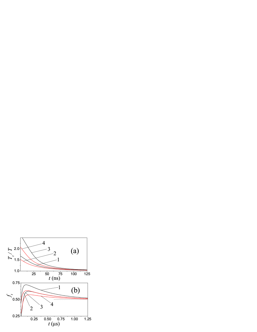
Figure 4: Temporal evolution of effective temperature, $T_{t}$ (a), and maximum distribution, $f_{t}$ (b), for different excitation conditions: (1) $\hbar\overline{\omega}=$60 meV and $I_{ex}=$0.21, (2) $\hbar\overline{\omega}=$60 meV and $I_{ex}=$0.1, (3) $\hbar\overline{\omega}=$120 meV and $I_{ex}=$0.052, and (4) $\hbar\overline{\omega}=$120 meV and $I_{ex}=$0.026.

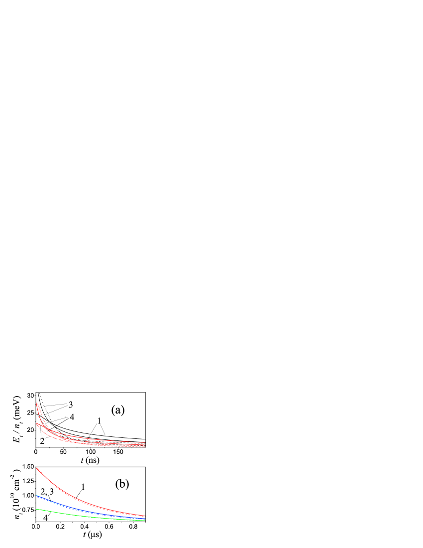
Figure 5: Energy per carrier (a) and concentration (b) versus time. Solid and dotted curves correspond to the cases ($i$) and ($ii$) , respectively; excitation conditions (1) - (4) are the same as in Fig. 4.

Numerical solution of the nonlinear system (11) is performed using the iteration procedure. In Fig. 4 we plot $T_{t}/T$ and $f_{t}$ versus time. Temperature relaxes to the equilibrium one during the energy relaxation times ($\lesssim$ 100 ns) while $f_{t}$, which is determined by the chemical potential $\mu_{t}$, relaxes to 1/2 over 1 $\mu$s (the recombination time scale), in analogy with the case ($i$). Notice, that after the fast energy relaxation, one obtains $f_{t}>$1/2 [dotted line in Fig. (4b)], i.e. the low-energy electron-hole pairs appear to be unstable. 19

Fig. 5 shows the plot of temporal evolutions of the energy per particle and concentration, $E_{t}/n_{t}$ and $n_{t}$ [see the definitions before Eq. (11)], for the cases ($i$) and ($ii$). The relaxation processes to the equilibrium (at nitrogen temperature, $E_{t\to\infty}/n_{t\to\infty}\simeq$14.5 meV and $n_{t\to\infty}\simeq 5.3\cdot 10^{9}$ cm^-2) occur during the same scales as in Figs. 3 and 4. The temporal dependencies of $n_{t}$ obtained for both cases are in good agreement (the carreir-carrier scattering does not change concentration) while $E_{t}$ demonstrates a different evolution for cases ($i$) and ($ii$) at $t<$50 ns. This is because of drift and decrease of photoexcited peak during the energy relaxation time, see Fig. 3.

IV Transient response

Here we turn to consideration of the response of photoexcited carriers on a probe radiation (reflection and transmission in the THz and mid-IR spectral regions) and on a weak dc electric field (photoconductivity). The transient electrodynamics of graphene is described using the time-dependent dynamic conductivity, $\sigma_{\omega t}$, which is caused by the collisionless interband transitions, see Appendix B. The transient photoconductivity is calculated by the use of the phenomenological model of momentum relaxation suggested in 13 .

IV.1 Reflection and transmission

To calculate the transient reflectance and transmittance of the graphene sheet placed at $z=0$ on the in-plane electric field ${\bf E}_{zt}\exp(-i\omega t)$ propagated along $0Z$, we apply the wave equation, see 20 and references therein. The induced current density, $\sigma_{\omega t}E_{z=0}$, is located around $z=0$ and direction of in-plane field ${\bf E}_{zt}$ is not essential due to the in-plane isotropy of the problem. Separating the incident radiation, $E_{in}e^{ik_{\omega}z}$, with the wave vector $k_{\omega}=\omega/c$, we write the field distribution outside of the graphene sheet in the form:

$$E_{zt}=\left\{\begin{array}[]{*{20}c}E_{in}e^{ik_{\omega}z}+E_{t}^{(t)}e^{-ik_{\omega}z},&{z<-0}\\ E_{t}^{(t)}e^{i\overline{k}_{\omega}z},&{z>+0}\end{array}\right.,$$ (15)

where $\overline{k}_{\omega}=\sqrt{\epsilon}\omega/c$ is the wave vector in the substrate with the dielectric permittivity $\epsilon$. The transmitted and reflected electric fields, $E_{t}^{(t)}$ and $E_{t}^{(r)}$, are determined from the boundary conditions at $z\to 0$ as follows:

$$\frac{E_{t}^{(t)}}{E_{in}}=\frac{2}{1+A_{\omega t}},~{}~{}~{}~{}\frac{E_{t}^{(t)}}{E_{in}}=\frac{1-A_{\omega t}}{1+A_{\omega t}}.$$ (16)

Here we introduce the dimensionless factor $A_{\omega t}=\sqrt{\epsilon}+(4\pi/c)\sigma_{\omega t}$. The reflection and transmission coefficients, $R_{\omega t}=|E_{t}^{(r)}|^{2}/E_{in}^{2}$ and $T_{\omega t}=|E_{t}^{(t)}|^{2}/E_{in}^{2}$, are written through $A_{\omega t}$ according to

$$R_{\omega t}=\left|\frac{1-A_{\omega t}}{1+A_{\omega t}}\right|^{2},~{}~{}~{}~{}~{}T_{\omega t}=\frac{4\sqrt{\epsilon}}{\left|1+A_{\omega t}\right|^{2}}.$$ (17)

Using $\sigma_{\omega t}$ determined by Eqs. (B3) and (B4), we consider below the differential changes in reflectivity and transmissivity, $(\Delta R/R)_{\omega t}=(R_{\omega t}-R_{\omega}^{(eq)})/R_{\omega}^{(eq)}$ and $(\Delta T/T)_{\omega t}=(T_{\omega t}-T_{\omega}^{(eq)})/T_{\omega}^{(eq)}$, which are written through the equilibrium reflection and transmission coefficients, $R_{\omega}^{(eq)}$ and $T_{\omega}^{(eq)}$.

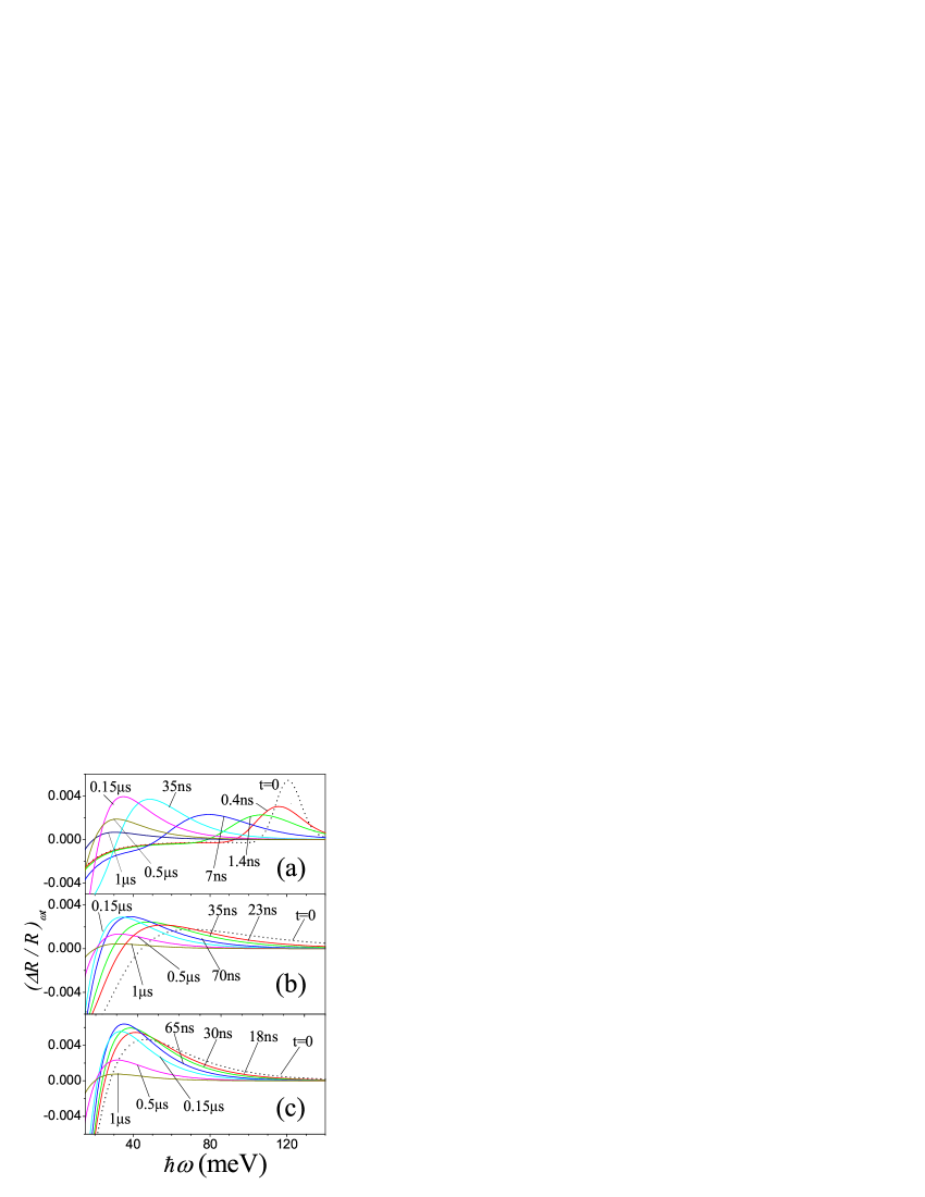
Figure 6: (a) Spectral dependencies of differential reflectivity, $(\Delta R/R)_{\omega t}$, for different delays (marked) at the excitation conditions: (a) $\hbar\overline{\omega}=$120 meV and $I_{ex}=0.052$ in the case ($i$), (b) $\hbar\overline{\omega}=$120 meV and $I_{ex}=$0.052 in the case ($ii$), and (c) $\hbar\overline{\omega}=$60 meV and $I_{ex}=$0.21 in the case ($ii$).

The evolution of the differential reflectivity for the cases ($i$) and ($ii$) are shown in Figs. 6a and 6b, 6c, respectively. If the Coulomb scattering is not effective [case ($i$)], the distribution of carriers relaxes during the energy relaxation time scale (around 10 ns, cf. with Fig. 3), when a quenching of photoexcited peak takes place (if $\hbar\omega$ is comparable with the peak energy). In case ($ii$) any peculiarities of the spectrsal dependencies at stort times are absent because the initial distribution is transformed into the quasiequilibrium one during times $\sim\tau_{cc}\to 0$. The further evolution of $(\Delta R/R)_{\omega t}$ is limited by the generation-recombination process and extended up to microseconds. In the THz spectral region ($\hbar\omega\geq$10 meV is considered here because we neglect the intraband relaxation), the differential reflectivity increases and changes a sign. In the high-energy region, $(\Delta R/R)_{\omega t}$ decreases monotonically with $\omega$ and $t$ and does not exceed $\sim 10^{-4}$ for the near-IR spectral region. Beside of this, the response is approximately proportional to the pumping intensity, $I_{ex}$, and $(\Delta R/R)_{\omega t}$ increases with increasing of the photoexcitation energy, $\hbar\overline{\omega}$ (cf. Figs. 6b and 6c).

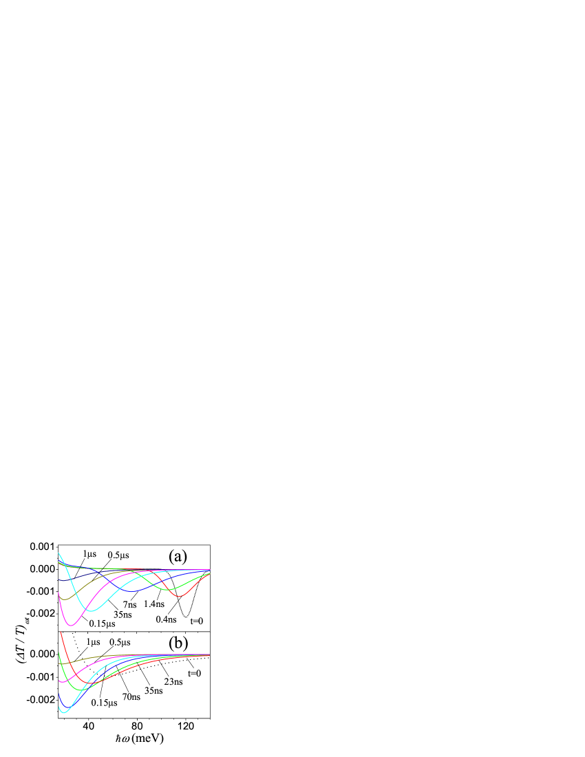
Figure 7: (a) Differential transmissivity, $(\Delta T/T)_{\omega t}$, versus $\hbar\omega$ and $t$ for cases ($i$) and ($ii$) [panels (a) and (b), respectively] at the same excitation conditions: $\hbar\overline{\omega}=$120 meV, $I_{ex}=$0.052.

In Fig. 7 we plot the differential transmissivity for the cases ($i$) and ($ii$) under the same excitation conditions. Once again, in the high-frequency region the differential transmissivity decreases slowly (during a microsecond time scale) and $(\Delta T/T)_{\omega t}$ does not exceed $\sim 10^{-4}$ for the near-IR spectral region. In the THz spectral region, $(\Delta T/T)_{\omega t}$ increses and changes the sing in the same manner as $(\Delta R/R)_{\omega t}$ (cf. Figs. 6 and 7). The dependencies on the excitation parameters ($I_{ex}$ and $\hbar\overline{\omega}$) are also similar to the reflectivity. Additionally, in case ($i$) a fast (at $t<$10 ns) quenching of the photoexcited peak contribution in the spectral region $\sim\hbar\Omega$ takes place.

IV.2 Photoconductivity

Finally, we consider the transient photoconductivity, i.e. the response of the photoexcited carriers to the weak dc electric field. Since the momentum relaxation is governed by elastic scattering mechanisms, 13 one can use the following expression for the dc conductivity $\sigma_{t}$:

$$\sigma_{t}=\sigma_{0}\left[2f_{p=0t}-\frac{l_{c}}{\hbar}\int_{0}^{\infty}dpf_{pt}\frac{\Psi^{\prime}(pl_{c}/\hbar)}{\Psi(pl_{c}/\hbar)^{2}}\right].$$ (18)

Here $l_{c}$ is the correlation length characterizing the disorder scattering and the function $\Psi(z)=e^{-z^{2}}I_{1}(z^{2})/z^{2}$ is written through the first order Bessel function of imaginary argument, $I_{1}(z)$. The normalized conductivity, $\sigma_{0}$, is introduced for the case of short-range scattering, when $l_{c}=0$. The distribution $f_{p=0t}$ is shown in Fig. 4b for the case ($ii$) while $2f_{p=0t}=1$ for the case ($i$). If $l_{c}=0$, one obtains $\sigma_{t}/\sigma_{0}=1$, i.e. there is no transient photoconductivity for the case ($i$); for the case ($ii$) one obtains $\sigma_{t}/\sigma_{0}=2f_{t}$ and the transient photoconductivity is clear from Fig. 4b.

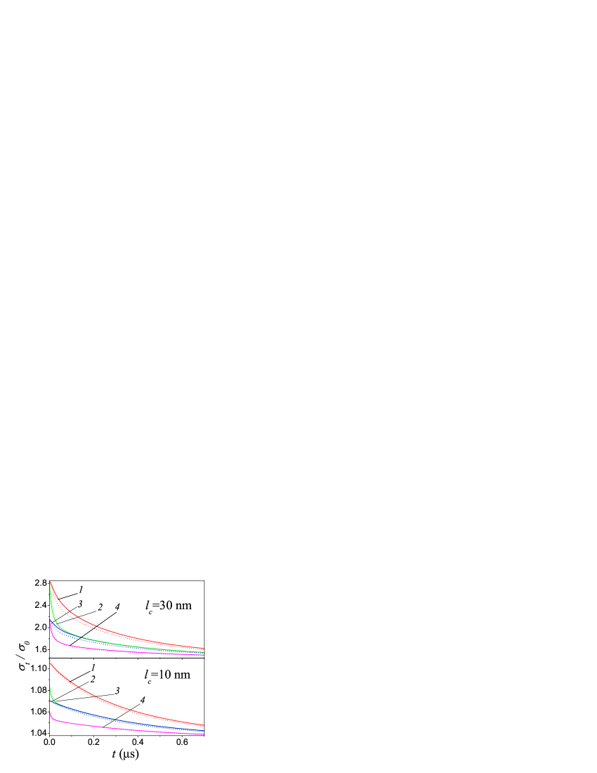
Figure 8: Temporal evolution of conductivity for excitation conditions (1)-(4) which are the same as in Fig. 4 for the correlation length $l_{c}=$30 nm and 10 nm. Solid and dashed curves are correspondent to the cases ($ii$) and ($i$).

If $l_{c}\neq 0$, the transient evolution of conductivity is shown in Fig. 8. For the definiteness, it was assumed that $l_{c}$=10 and 30 nm and variations of $\sigma_{t}$ are increased with $l_{c}$ essentially due to contribution of high-energy carriers. Similar to Sec. IVA, one can separate two stages of evolution: the fast decrease of $\sigma_{t}$ due to energy relaxation (up to $\sim 30\div 50$ ns for the conditions considered) and the slow quenching of $\sigma_{t}$ due to carrier recombination. If $t>1~{}\mu$s, the conductivity approaches to the equilibrium values: $\sigma_{t\to\infty}/\sigma_{0}=$1.445 if $l_{c}$=30 nm and $\sigma_{t\to\infty}/\sigma_{0}=$1.035 if $l_{c}$=10 nm. Since the transient conductivity can be measured for the subnanosecond time scale 21 , such a scheme can be used for verification both energy relaxation and recombination mechanisms.

V Concluding remarks

To summarize, we have considered both the interband ultrafast photoexcitation and the relaxation dynamics of the carriers in an intrinsic graphene. In contrast to the measurements 3 ; 4 ; 5 ; 6 and calculations 8 ; 9 performed, where the evolution corresponds to the subpicosecond time scales due to the opticlal phonon contribution, here we consider the slow relaxation of the low-energy carriers. The distribution of carriers at $T=$77 K is obtained for the limiting cases with negligible or dominating intercarrier scattering when the energy relaxation and generation-recombination processes are caused by the quasielastic acoustic phonon scattering and thermal radiation, respectively. The initial distribution is obtained in the framework of the linear, with respect to pumping, approximation for the collisionless regime of the interband transitions. The transient optical response on the probe radiation (transmission and reflection) as well as on the weak dc field (transient photoconductivity) appears to be strongly dependent on the relaxation and recombination dynamics of carriers.

Next, we discuss the assumptions made. The main restrictions of the results presented are the consideration of the low-energy carriers, when the interaction with optical phonons is unessential, and the single generation-recombination mechanism (due to thermal radiation) is taken into account. These conditions are realized at low temperatures under the mid-IR ultrafast excitation 17 of the clean sample (e.g. suspended graphene 22 ). Such an approach can be used for the case of optical interband excitation, when the low-energy initial distrbution, with a phenomenological broadening, is formed after the cascade process of optical phonon emission. The consideration is restricted by the radiative recombination (the Auger processes are forbidden due to the symmetry of electron-hole states 23 ), with the characteristic time scales up to microseconds. Any visible contribution of other generation-recombination mechanism (e.g., because of disorder-induced interband transitions with acoustic phonons, or under intercarrier scattering) leads to fast decrease of photoresponse. Such a regime requires an additional investigation but the quasielastic energy relaxation stage is described by the presented results.

The rest of assumptions are rather standard. The consideration in Sec. III is limited by the simple cases ($i$) and ($ii$), with and without the intercarrier scattering. The main peculiarities of the response under consideration are similar for both cases but the complete description of the nonequilibrium carriers had been performed neither under optical excitation, nor under high dc field, see 18 ; 24 and Refs. therein. The description of the momentum relaxation in Sec. IV is based on the phenomenological model of Ref. 13. The utilization of the quasielastic energy scattering and the collisionless interband photoexcitation appear to be rather natural. The listed assumptions do not change either the character of the response or the numerical estimates.

In closing, the peculiarities of the transient optical response (transmission and reflection) as well as of the transient photoconductivity appear to be useful tool in order to verify the relaxation and generation-recombination mechanisms of carriers. Thus, in addition to the recently obtained experimental results 3 ; 4 ; 5 ; 6 ; 7 measurements under mid-IR excitation and at low-temperature will be useful for characterization of graphene.

Appendix A Generation rate

Below we describe the interband carrier excitation under ultrafast mid-IR pumping ${\bf E}_{t}\exp(-i\Omega t)$ for the collisionless case, when $\tau_{p}$ is shorter than relaxation times. The photogeneration rate into the $\alpha$-state is based on the general expression (see 1 and Sec. 54 in Ref. 12)

$$G_{\alpha t}=2Re\left(\frac{e}{\hbar\Omega}\right)^{2}\int\limits_{-\infty}^{0}d\tau e^{\lambda\tau-i\Omega\tau}~{}~{}~{}~{}~{}~{}~{}~{}~{}$$ (19)

$$\times\left\langle\alpha\left|\left[e^{i\hat{h}\tau/\hbar}\left[\left({\bf E}_{t+\tau}\cdot{\bf\hat{v}}\right),\hat{\rho}_{t+\tau}\right]e^{-i\hat{h}\tau/\hbar},\left({\bf E}_{t}\cdot{\bf\hat{v}}\right)^{+}\right]\right|\alpha\right\rangle,$$

where $\hat{\rho}_{t}$ is the density matrix, $\hat{\bf v}$ is the velocity operator, and $\lambda\to+0$. Since the collisionless regime of photoexcitation, we calculate (A1) with the use of the free states $|l{\bf p}\rangle$ and the energy $\varepsilon_{lp}$ where $l=\pm 1$ stands for $c$- or $v$-bands and $\bf p$ is the 2D momentum. Neglecting the nondiagonal components of the density matrix $\hat{\rho}_{t}$ and using the distribution functions $f_{l{\bf p}t}$, one obtains the generation rate

$$G\{f|1{\bf p}t\}=\left(\frac{e}{\hbar\Omega}\right)^{2}\int\limits_{-\infty}^{0}d\tau e^{\lambda\tau-i\Omega\tau}e^{i(\varepsilon_{1p}-\varepsilon_{-1p})\tau/\hbar}$$

$$\times\langle 1{\bf p}|({\bf E}_{t+\tau}\cdot{\bf\hat{v}})|-1{\bf p}\rangle\langle-1{\bf p}|({\bf E}_{t}\cdot{\bf\hat{v}})^{+}|1{\bf p}\rangle~{}~{}~{}~{}~{}$$ (20)

$$\times\left(f_{-1{\bf p}t+\tau}-f_{1{\bf p}t+\tau}\right)+c.c.~{},$$

moreover $G\{f|-1{\bf p}t\}=-G\{f|1{\bf p}t\}$ according to the particle concervation law. Next, we separate the envelope form-factor $w_{t}$ using ${\bf E}_{t}={\bf E}w_{t}$ and take into account the in-plane isotropy of the problem, when one arrives to the averaged matrix element $\overline{\left|\left\langle+1{\bf p}\left|({\bf E}\cdot{\bf\hat{v}})\right|-1{\bf p}\right\rangle\right|^{2}}=(Ev_{W})^{2}/2$. As a result, we obtain the in-plane isotropic generation rate $G\{f|pt\}=\pm G\{f|\pm lpt\}$ in the following form:

$$G\{f|pt\}=\left(\frac{eEv_{W}}{\hbar\Omega}\right)^{2}\frac{w_{t}}{2}\int\limits_{-\infty}^{0}d\tau w_{t+\tau}e^{\lambda\tau-i\Omega\tau}$$

$$\times e^{i(2v_{W}p)\tau/\hbar}\left(f_{-1{\bf p}t+\tau}-f_{1{\bf p}t+\tau}\right)+c.c.~{}.$$ (21)

Finally, using the electron-hole representation and replacing the filling factor here by $(1-2f_{pt})$, we arrive to Eq. (2).

Appendix B Dynamic conductivity

The response of graphene on the in-plane probe field ${\bf E}\exp(-i\omega t)$ is described by the dynamic conductivity 20 ; 25

$$\sigma_{\omega t}\approx i\frac{2(ev_{W})^{2}}{\omega L^{2}}\sum\limits_{\bf p}(1-2f_{pt})~{}~{}~{}~{}$$ (22)

$$\times\left(\frac{1}{\hbar\omega+2v_{W}p+i\lambda}-\frac{1}{\hbar\omega-2v_{W}p+i\lambda}\right)$$

with $\lambda\to+0$. The parametric time dependency of $\sigma_{\omega t}$ is valid if the time scales under consideration exceed $\omega^{-1}$. It is convenient to separate the time-independent contribution, $\overline{\sigma}_{\omega}$, described the undoped graphene in the absence of photoexcitation, when $f_{pt}$ vanishes. Using the energy conservation law one obtains ${\rm Re}\overline{\sigma}_{\omega}=e^{2}/4\hbar$. In the framework of the Weyl-Wallace model, the ${\rm Im}$-contribution into $\overline{\sigma}_{\omega}$ appears to be divergent at $p\to\infty$. It is convenient to approximate ${\rm Im}\overline{\sigma}_{\omega}$ as a sum of $\propto\omega^{-1}$ and $\propto\omega$ terms, which correspond to the contributions of the virtual interband transitions and the ion background, correspondingly. As a result, we obtain:

$${\rm Im}\overline{\sigma}_{\omega}\approx\frac{e^{2}}{\hbar}\left(\frac{\varepsilon_{m}}{\hbar\omega}-\frac{\hbar\omega}{\varepsilon_{i}}\right),$$ (23)

where the characteristic energies, $\varepsilon_{m}\simeq$0.1 eV, and $\varepsilon_{i}\simeq$ 6.8 eV are correspondent to the recent measurements of the graphene optical spectrum. 26

Next, substituting the time-dependent distribution $f_{pt}$ obtained in Sec. III into the dynamic conductivity (B1) one transforms the real and imagional parts of $\sigma_{\omega t}$ as follows

$${\rm Re}\sigma_{\omega t}=\frac{e^{2}}{4\hbar}\left[1-2F\left(p_{\omega},t\right)\right],~{}~{}~{}~{}~{}~{}~{}$$ (24)

$${\rm Im}\sigma_{\omega t}={\rm Im}\overline{\sigma}_{\omega}-\frac{e^{2}}{\pi\hbar}{\cal P}\int\limits_{0}^{\infty}\frac{dyy^{2}}{1-y^{2}}F(p_{\omega}y,t).$$

Here $\cal P$ means the principal value of integral. We also introduced the function $F(p,t)=f_{pt}$ for the case ($i$) and

$$F\left(p_{\omega}y,t\right)=\frac{f_{t}}{\exp[(\hbar\omega/T_{t})y](1-f_{t})+f_{t}}$$ (25)

for the case ($ii$), when $\sigma_{\omega t}$ is determined both the effective temperature and the carrier concentration, $T_{t}$ and $f_{t}$.

References

- (1) J. Shah, Ultrafast Spectroscopy of Semiconductors and Semiconductor Nanostructures, (Springer, New York, 1996); F. T. Vasko and A. V. Kuznetsov, Electron States and Optical Transitions in Semiconductor Heterostructures (Springer, New York, 1998).
- (2) E. M. Lifshitz, L. P. Pitaevskii, and V. B. Berestetskii, Quantum Electrodynamics, (Butterworth-Heinemann, Oxford 1982); P. R. Wallace, Phys. Rev. 71, 622 (1947).
- (3) J. M. Dawlaty, S. Shivaraman, M. Chandrashekhar, F. Rana, and M. G. Spencer Appl. Phys. Lett. 92, 042116 (2008).
- (4) D. Sun, Z.-K. Wu, C. Divin, X. Li, C. Berger, W. A. de Heer, P. N.First, and T. B. Norris, Phys. Rev. Lett. 101, 157402 (2008).
- (5) P. A. George, J. Strait, J. Dawlaty, S. Shivaraman, Mvs. Chandrashekhar, F. Rana, and M. G. Spencer, Nanoletters 8, 4248 (2008).
- (6) R. W. Newson, J. Dean, B. Schmidt, and H. M. van Driel, Opt. Exp. 17, 2326 (2009).
- (7) H. Wang, J. H. Strait, P. A. George, S. Shivaraman, V. B. Shields, Mvs Chandrashekhar, J. Hwang, F. Rana, M. G. Spencer, C. S. Ruiz-Vargas, and J. Park, arXiv:0909.4912
- (8) S. Butscher, F. Milde, M. Hirtschulz, E. Malic, and A. Knorr, Appl. Phys. Lett. 91, 203103 (2007).
- (9) F. Rana, P. A. George, J. H. Strait, J. Dawlaty, S. Shivaraman, Mvs Chandrashekhar, and M. G. Spencer, Phys. Rev. B 79, 115447 (2009.
- (10) F. T. Vasko and V. Ryzhii, Phys. Rev. B 77, 195433 (2008); A. Satou, F. T. Vasko and V. Ryzhii, Phys. Rev. B 78, 115431 (2008).
- (11) R. Bistritzer and A. H. MacDonald, Phys. Rev. Lett. 102, 206410 (2009).
- (12) F. T. Vasko and O. E. Raichev, Quantum Kinetic Theory and Applications (Springer, New York, 2005).
- (13) F. T. Vasko and V. Ryzhii, Phys. Rev. B 76, 233404 (2007).
- (14) The form-factor is normalized according to the condition . The shape of normalized form-factor has little effect on the transient photoexcitation under consideration because the ultrafast response is determined fundamentally by the pulse duration, .
- (15) Here we use the characteristic velocities 2.5 cm/s (for the nitrogen temperature) and 41.6 cm/s (for graphene sheet placed between SiO2 substrate and cover layer), see 10 .
- (16) D. Potter, Computational Physics (J. Wiley, London, 1973).
- (17) T. Elsaesser and M. Woerner, Physics Reports 321, 253 (1999).
- (18) O. G. Balev, F. T. Vasko and V. Ryzhii, Phys. Rev. B 79, 165432 (2009).
- (19) According to Eq.(B3), the negative interband absorption () takes place, if , see 10 and Refs. therein. This low-energy instability is suppressed due to an effective intraband (Drude) absorption.
- (20) L. A. Falkovsky, Phys. Usp. 51, 887 (2008); T. Stauber, N. M. R. Peres, and A. K. Geim, Phys. Rev. B78, 085432 (2008); M. V. Strikha and F. T. Vasko, submitted.
- (21) T. Yao, K. Inagaki, and S. Maekawa, in Proceedings of the 11th International Conference on the Physics of Semiconductors (Polish Scientific Publishers, Warszawa, 1972), Vol. 1, p. 417.
- (22) G. Li, A. Luican, and E. Y. Andrei, Phys. Rev. Lett. 102, 176804 (2009); P. Neugebauer, M. Orlita, C. Faugeras, A. L. Barra, and M. Potemski, Phys. Rev. Lett. 103, 136403 (2009).
- (23) M. S. Foster and I. L. Aleiner, Phys. Rev. B 79, 085415 (2009).
- (24) A. Akturka and N. Goldsman, J. Appl. Phys. 103, 053702 (2008); R. S. Shishir and D. K. Ferry, J. Phys.: Condens. Matter, 21, 344201 (2009).
- (25) R. R. Nair, P. Blake, A. N. Grigorenko, K. S. Novoselov, T. J. Booth, T. Stauber, N. M. R. Peres, and A. K. Geim, Science 320, 1308 (2008); T. Stauber, N. M. R. Peres, and A. K. Geim, Phys. Rev. B78, 085432 (2008); K. F. Mak, M. Y. Sfeir, Y. Wu, C. H. Lui, J. A. Misewich, and T. F. Heinz, Phys. Rev. Lett. 101, 196405 (2008).
- (26) M. Bruna and S. Bonilla, Appl. Phys. Lett. 94, 031901 (2009).