Abstract

For an integer $d\geq 1$, let $\tau(d)$ be the smallest integer with the following property: If ${\bf v}_{1},{\bf v}_{2},\ldots,{\bf v}_{t}$ is a sequence of $t\geq 2$ vectors in $[-1,1]^{d}$ with ${\bf v}_{1}+{\bf v}_{2}+\cdots+{\bf v}_{t}\in[-1,1]^{d}$, then there is a set $S\subseteq\{1,2,\ldots,t\}$ of indices, $2\leq|S|\leq\tau(d)$, such that $\sum_{i\in S}{\bf v}_{i}\in[-1,1]^{d}$. The quantity $\tau(d)$ was introduced by Dash, Fukasawa, and Günlük, who showed that $\tau(2)=2$, $\tau(3)=4$, and $\tau(d)=\Omega(2^{d})$, and asked whether $\tau(d)$ is finite for all $d$.

Using the Steinitz lemma, in a quantitative version due to Grinberg and Sevastyanov, we prove an upper bound of $\tau(d)\leq d^{d+o(d)}$, and based on a construction of Alon and Vũ, whose main idea goes back to Håstad, we obtain a lower bound of $\tau(d)\geq d^{d/2-o(d)}$.

These results contribute to understanding the master equality polyhedron with multiple rows defined by Dash et al., which is a “universal” polyhedron encoding valid cutting planes for integer programs (this line of research was started by Gomory in the late 1960s). In particular, the upper bound on $\tau(d)$ implies a pseudo-polynomial running time for an algorithm of Dash et al. for integer programming with a fixed number of constraints. The algorithm consists in solving a linear program, and it provides an alternative to a 1981 dynamic programming algorithm of Papadimitriou.

1 Introduction

Let $d\geq 1$ and let us consider the unit cube $[-1,1]^{d}$; we will call it the box in this paper. We want to construct a large number $t$ of vectors ${\bf v}_{1},{\bf v}_{2},\ldots,{\bf v}_{t}$, each of them lying in the box, such that

1. the sum ${\bf s}={\bf v}_{1}+{\bf v}_{2}+\cdots+{\bf v}_{t}$ also lies in the box, but

2. for every proper subset $S\subset[t]$ of indices with $2\leq|S|<t$, the sum $\sum_{i\in S}{\bf v}_{i}$ lies outside the box (we have to exclude $|S|=1$, since every ${\bf v}_{i}$ itself does lie in the box).

So we are interested in long minimal sequences with sum in the box. Let $\tau(d)$ denote the largest $t$ such that a minimal sequence as above exists (it is easy to see that the definition in the abstract, although phrased differently, is actually equivalent).

In order to illustrate this definition, let us check that $\tau(2)=2$. We have $\tau(d)\geq 2$ for all $d$ by definition. For proving $\tau(d)\leq 2$, we need to show that in every sequence ${\bf v}_{1},\ldots,{\bf v}_{t}\in[-1,1]^{2}$ with sum in the box there are two vectors with sum in the box.

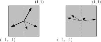
Figure 1: Illustration to the proof of $\tau(2)=2$: Either we find two vectors in opposite quadrants, or one of the coordinates has the same sign for all the vectors and can be ignored.

If two of the vectors lie in opposite quadrants, as in Fig. 1 left, then their sum is in the box and we are done. Otherwise, some two neighboring quadrants have to be empty, which means that one of the two coordinates has the same sign for all the ${\bf v}_{i}$; w.l.o.g. we may assume that all the ${\bf v}_{i}$ have a positive $y$-coordinate. Then the $y$-coordinate can be ignored (since it lies in $[-1,1]$ for the sum of any subsequence), and it suffices to show that the sum of some two of the $x$-coordinates lies in $[-1,1]$. In other words, it now suffices to check that $\tau(1)=2$, which we leave to the reader.

An example showing $\tau(3)\geq 4$ is the sequence $(1,1,\frac{2}{3})$, $(1,-\frac{2}{3},-1)$, $(-\frac{2}{3},1,-1)$, $(-\frac{2}{3},-\frac{2}{3},\frac{2}{3})$.

The quantity $\tau(d)$ was introduced by Dash, Fukasawa, and Günlük [5] in the context of integer programming (we will discuss the motivation later). They found the values $\tau(2)=2$ and $\tau(3)=4$, and they asked whether $\tau(d)$ is finite for all $d$. We provide a positive answer, with the following upper bound:

Theorem 1.1

For all $d\geq 1$ we have $\tau(d)<4(2d)^{d}.$

Our proof, presented in Section 2 below, is based on the so-called Steinitz lemma, in a quantitative version due to Grinberg and Sevastyanov [7].

We also show that the upper bound is not far from the truth.

Theorem 1.2

There is a constant $c>0$ such that

$$\tau(d)\geq(cd)^{d/2}$$

for all $d$ that are powers of $2$.

The proof, given in Section 2 is based on a construction of very ill-conditioned square matrices with $\pm 1$ entries, due to Alon and Vũ [2] (the basic idea going back to Håstad [8]). It seems likely that the lower bound could be extended to all $d$, instead of just powers of $2$, but this might need a careful analysis of another construction from [2].

There is a natural and, in our opinion, interesting variant of the quantity $\tau(d)$, where one again considers sequences ${\bf v}_{1},\ldots,{\bf v}_{t}\in[-1,1]^{d}$ satisfying (i) and (ii) above, but the ${\bf v}_{i}$ are restricted to only $\pm 1$ vectors. Let $\tau_{\pm 1}(d)$ denote the corresponding maximum length of such a sequence; we have $\tau_{\pm 1}(d)\leq\tau(d)$ by definition. We obtain the following slightly weaker lower bound:

Theorem 1.3

There is a constant $c>0$ such that $\tau_{\pm 1}(d)\geq(cd)^{d/4}$ for all $d$ that are powers of $2$.

The IP connection. The quantity $\tau(d)$ has been motivated by a connection to an algorithm for integer programming.

Let us consider an integer program in the form

$$\min\{{\bf c}^{T}{\bf x}:{\bf x}\in{\mathbb{Z}}^{\ell},A{\bf x}={\bf b},{\bf x}\geq{\bf 0}\},$$ (1)

where $A$ is an $m\times\ell$ integer matrix, ${\bf c}\in{\mathbb{Z}}^{\ell}$, and ${\bf b}\in{\mathbb{Z}}^{m}$. This optimization problem is well-known to be NP-hard even for $m=1$, i.e., for a single equality constraint (this follows, e.g., from the hardness of the knapsack problem). On the other hand, Papadimitriou [9] proved that if $m$ is fixed and the entries of $A$ and ${\bf b}$ are small integers, bounded in absolute value by a parameter $N$, then the integer program can be solved in pseudo-polynomial time. That is, the running time can be bounded by a polynomial in $\ell$ and $N$ (and the input size of ${\bf c}$); the polynomial depends on $m$.

Papadimitriou’s algorithm is based on dynamic programming (also see Schrijver [10] for a description); it searches for a shortest path in an auxiliary graph. Dash et al. [5] provided a completely different algorithm for the same problem, which consists in solving a linear program over an auxiliary polyhedron (the so-called polaroid). They obtained a pseudo-polynomial bound for the number of inequalities in the linear program, and thus also for the running time, but only for input integer programs with $m\leq 3$ constraints (actually, they handled the case of $m=1$ constraint earlier in [4]). To get pseudo-polynomiality for larger $m$, they needed the finiteness of $\tau(m)$. Thus, combined with our Theorem 1.1, their algorithm provides an alternative to Papadimitriou’s method.

We won’t review the algorithm here; we only recall some of the key concepts, and then we indicate how $\tau(m)$ is related to the linear program.

The approach of Dash et al. goes back to a paper of Gomory [6]. In that remarkable work, which introduced several important ideas of modern polyhedral combinatorics, Gomory defined a certain “universal” polyhedron, the master cyclic group polyhedron, whose faces encode all instances of integer programs in a certain class (see, e.g., [1] for an introduction). Dash et al. [5] use the somewhat related concept of the master equality polyhedron $K^{m}(N,{\bf b})$, which we recall below. For $m=1$, it was introduced in an earlier paper by Dash et al. [4], who attribute its origin to a 2005 talk of Uocha, and it contains as a face Gomory’s master cyclic group polyhedron, as well as the master knapsack polyhedron of Araóz.

Let

$$I:=\{-N,-N+1,\ldots,N\}^{m},$$

and let ${\bf b}\in I$ be a vector corresponding to the right-hand side in (1). Then the master equality polyhedron resides in ${\mathbb{R}}^{I}$ and it is defined as

$$K^{m}(N,{\bf b}):={\mathop{\rm conv}\nolimits}\{{\bf x}\in{\mathbb{Z}}^{I}:\sum_{{\bf v}\in I}x_{\bf v}{\bf v}={\bf b},{\bf x}\geq{\bf 0}\}.$$

It turns out that the separation problem for the integer program (1) can be reduced to the separation problem for $K^{m}(N,{\bf b})$.

For $m=1$, Dash et al. [4] obtained a description of a nontrivial polar $T$ of $K^{1}(N,b)$, i.e. a polyhedron whose vertices correspond to the nontrivial facets of $K^{1}(N,b)$, and thus reduced the separation problem for $K^{1}(N,b)$ to optimizing a linear function over $T$. It is important that $T$ is described by polynomially many linear constraints.

In [5] Dash et al. describe an example showing that for $m\geq 2$, a sufficiently compact description of a nontrivial polar of $K^{m}(N,{\bf b})$ may be very hard to find, if it exists at all. However, they defined the new notion of a polaroid of $K^{m}(N,{\bf b})$, and proved that the separation problem for $K^{m}(N,{\bf b})$ can be reduced to a suitable linear program over the polaroid. Again, one needs a polynomial bound on the number of constraints in this linear program, and here $\tau(m)$ enters the game.

The variables of the linear program are $\pi_{{\bf v}}$ for all integer vectors ${\bf v}\in I$, and the main kind of constraints in it are subadditivity constraints of the form

$$\pi_{{\bf v}_{1}}+\cdots+\pi_{{\bf v}_{t}}\geq\pi_{{\bf v}_{1}+\cdots+{\bf v}_{t}},$$ (2)

where ${\bf v}_{1},\ldots,{\bf v}_{t}\in I$ are vectors whose sum also lies in $I$. Now suppose, for example, that ${\bf v}_{1}+{\bf v}_{2}+\cdots+{\bf v}_{k}$ also lies in $I$, for some $k$ with $2\leq k<t$. Then (2) is a consequence of the subadditivity constraints

$$\pi_{{\bf v}_{1}}+\cdots+\pi_{{\bf v}_{k}}\geq\pi_{{\bf v}_{1}+\cdots+{\bf v}_{k}}\ \ \mbox{and}\ \ \pi_{{\bf v}_{1}+\cdots+{\bf v}_{k}}+\pi_{{\bf v}_{k+1}}+\cdots+\pi_{{\bf v}_{t}}\geq\pi_{{\bf v}_{1}+\cdots+{\bf v}_{t}}.$$

Similarly, whenever there is an $S\subset[t]$ with $2\leq|S|<t$ and $\sum_{i\in S}{\bf v}_{i}\in I$, the constraint (2) is implied by subadditivity constraints with a smaller number of terms. Thus, it is sufficient to consider only subadditivity constraints with $t\leq\tau(m)$.

The quantity $\tau(m)$ gives only an upper bound on the number of non-redundant subadditivity constraints. Dash et al. [5] define another quantity $k^{*}(m)\leq\tau(m)$, which is related to the number of non-redundant constraints more directly. In Corollary 3.3 we will give a lower bound of $(cm)^{m/4}$ for $k^{*}(m)$, which shows that it is not much smaller than $\tau(m)$.

2 The Upper Bound

Let $B\subset{\mathbb{R}}^{d}$ be a $d$-dimensional closed convex body symmetric about ${\bf 0}$ (in other words, the unit ball of a norm on ${\mathbb{R}}^{d}$). Riemann and Lévy in the 19th century raised the question of whether there exists a number $m=m(B)$, depending only on $B$, such that the vectors of an arbitrary finite set (or multiset) $V\subset B$ with $\sum_{{\bf v}\in V}{\bf v}={\bf 0}$ can be ordered into a sequence ${\bf v}_{1},{\bf v}_{2},\ldots,{\bf v}_{n}$ so that each of the partial sums ${\bf v}_{1}+{\bf v}_{2}+\cdots+{\bf v}_{k}$, $1\leq k\leq n$, belongs to the expanded body $mB=\{m{\bf x}:{\bf x}\in B\}$. The first complete proof of a positive answer was given by Steinitz [11]. The strongest known quantitative version, with $m(B)=d$ for all bodies in ${\mathbb{R}}^{d}$, is due to Grinberg and Sevastyanov [7] (their beautiful proof can also be found in Bárány’s survey [3, Theorem 2.1]).

Theorem 2.1 (Steinitz lemma)

Let $B$ be a symmetric convex body in ${\mathbb{R}}^{d}$, and let $V\subset B$ be a finite set (or multiset) of vectors satisfying $\sum_{{\bf v}\in V}{\bf v}=0$. Then there is an ordering ${\bf v}_{1},{\bf v}_{2},\mathellipsis,{\bf v}_{n}$ of the elements of $V$ such that for all $k=1,2,\ldots,n$, we have $\sum_{i=1}^{k}{\bf v}_{i}\in dB$.

Proof of Theorem 1.1. Given a collection of $t$ vectors in the box whose sum also lies in the box, and assuming $t\geq t_{0}:=4(2d)^{d}$, we want to find a proper subcollection with sum in the box.

Here it will be more convenient to regard the given collection of $t$ vectors as a multiset $W$ (rather than as a sequence)—later we will obtain suitable ordering of the vectors in $W$ from the Steinitz lemma.

Thus, $W$ is a multiset of $t$ vectors; we let ${\bf s}:=\sum_{{\bf v}\in W}{\bf v}\in[-1,1]^{d}$ be their sum. We apply the Steinitz lemma as above with $B=[-1,1]^{d}$ and $V:=W\cup\{-{\bf s}\}$ (this is again a multiset, with $t+1$ vectors). This yields an ordering

$${\bf v}_{1},{\bf v}_{2},\ldots,{\bf v}_{i},-{\bf s},{\bf v}_{i+1},\ldots,{\bf v}_{t}$$

such that the sum of the first $k$ terms lies in $dB$ for every $k=1,2,\ldots,t+1$.

First, let us assume that the “artificial” element $-{\bf s}$ falls in the second half of the above sequence; that is, $i\geq t/2\geq t_{0}/2$. Let us subdivide the blown-up cube $dB$, whose side length is $2d$, into $(2d)^{d}$ cubes of side $1$, of the form $[0,1]^{d}+{\bf z}$, ${\bf z}\in\{-d,-d+1,\ldots,d-1\}^{d}$.

Let ${\bf s}_{k}:={\bf v}_{1}+\cdots+{\bf v}_{k}$ be the $k$th partial sum, $k=0,1,\ldots,t_{0}/2$, and let us consider every second of these, i.e., the points ${\bf s}_{0},{\bf s}_{2},{\bf s}_{4},\ldots,{\bf s}_{t_{0}/2}$. These are more than $t_{0}/4=(2d)^{d}$ points in $dB$, and so some two of them, ${\bf s}_{2i}$ and ${\bf s}_{2j}$, $0\leq i<j\leq t_{0}/4$, fall in the same cube $[0,1]^{d}+{\bf z}$.

Then the difference ${\bf s}_{2j}-{\bf s}_{2i}$ lies in the box. At the same time, it equals

$${\bf v}_{2i+1}+{\bf v}_{2i+2}+\cdots+{\bf v}_{2j},$$

and so we have found the desired proper submultiset of $W$ with sum in the box (and with at least two elements).

It remains to deal with the case when the artificial element $-{\bf s}$ lies in the first half of the sequence—then we use the same kind of argument as above for the second half. Theorem 1.1 is proved.   $\Box$

3 Lower bounds

All of our lower bounds are based on results of Alon and Vũ [2]. The main theme of that paper are ill-conditioned matrices with $\pm 1$ entries (or $0/1$ entries; these two settings are not very different).

Let us consider a nonsingular $d\times d$ matrix $A$ whose entries are $+1$’s and $-1$’s, and let $\chi(A)$ be the maximum of the absolute values of the entries of $A^{-1}$; the larger $\chi(A)$, the more ill-conditioned the matrix $A$ is. Let $\chi(d):=\max_{A}\chi(A)$, where the maximum is over all $d\times d$ nonsingular $\pm 1$ matrices.

Alon and Vũ showed that $\chi(d)=d^{d/2+o(d)}$ and gave several interesting applications. The main achievement was the (surprisingly large) lower bound, which was obtained by an explicit construction. For that purpose, Alon and Vũ modified and extended a construction of Håstad [8], which was formulated in a different setting, namely, in the language of threshold gates.

In this section we will provide three lower bound constructions for vectors in the box. The first construction is the simplest: It follows rather directly from a result explicitly stated in [2], but it loses a factor of two in the dimension, leading only to the lower bound of $\tau(d)\geq d^{d/4-o(d)}$. Then we give another, different and more complicated construction, which gives $\tau(d)\geq d^{d/2-o(d)}$ and proves Theorem 1.2, and finally, we modify the latter construction so that only $\pm 1$ vectors are used, obtaining Theorem 1.3.

Large quantities. In order to avoid boring formulas or repetitive phrases, we introduce the following piece of terminology. If $Q=Q(d)$ is some quantity in the forthcoming constructions, depending on $d$, we say that $Q$ is large if there is a constant $c>0$ such that $|Q|\geq(cd)^{d/2}$ holds for all of the considered values of $d$ (in the first construction we will consider all $d$, while in the second and third only powers of two). In particular, we note that a large quantity can be either positive or negative.

We note that being large is immune to division by exponential factors; e.g., if some $Q$ is large, then $Q/2^{d}$ is large as well.

3.1 The First Construction

Here we use the following result of Alon and Vũ:

Proposition 3.1 ([2, Proposition 3.4.3])

For every $d\geq 1$, there exists a $d\times(d+1)$ matrix $C$ of rank $d$ with entries $+1$ and $-1$ such that any nonzero integral solution ${\bf z}$ of the system $C{\bf x}={\bf 0}$ has at least one large component.

The construction. The following construction will show that $\tau(2d)$ is large (for all $d$), or in other words, that $\tau(d)\geq(cd)^{d/4}$.

Let $C$ be the $d\times(d+1)$ matrix as in Proposition 3.1. Since the system $C{\bf x}={\bf 0}$ is homogeneous, with rational coefficients, and has fewer equations than unknowns, there exist nonzero integral solutions.

Let ${\bf z}\in{\mathbb{Z}}^{d+1}$ be a nonzero integral solution of $C{\bf x}={\bf 0}$ with the smallest possible $L_{1}$ norm, i.e., minimizing $\|{\bf z}\|_{1}=\sum_{j=1}^{d+1}|z_{j}|$. Let us set $t:=\|{\bf z}\|_{1}$; by the above, $t=t(d)$ is large.

After possibly flipping the signs of some of the columns of $C$, we may assume that all components of ${\bf z}$ are nonnegative. Let ${\bf c}_{j}$ denote the $j$th column of $C$, and let ${\bf w}_{1},{\bf w}_{2},\ldots,{\bf w}_{t}$ be an (auxiliary) sequence of vectors containing $z_{j}$ copies of each ${\bf c}_{j}$, $j=1,2,\ldots,d+1$.

The ${\bf w}_{i}$ are vectors in the box (even $\pm 1$ vectors), and we have $\sum_{i=1}^{t}{\bf w}_{i}=\sum_{j=1}^{d+1}z_{j}{\bf c}_{j}=C{\bf z}={\bf 0}$.

It is also easy to see that no proper subsequence of the ${\bf w}_{i}$ has sum in the interior of the box. Indeed, the sum of any subsequence is an integral vector, so if it lies in $(-1,1)^{d}$, it has to be ${\bf 0}$. But choosing a proper subsequence of the ${\bf w}_{i}$ corresponds to choosing multiplicities $z^{\prime}_{1},\ldots,z^{\prime}_{d+1}$, with $z^{\prime}_{j}\leq z_{j}$ for all $j$ and with at least one of the inequalities strict. So a proper subsequence with zero sum corresponds to a nontrivial solution ${\bf z}^{\prime}$ of $C{\bf z}^{\prime}={\bf 0}$ with $\|{\bf z}^{\prime}\|_{1}<t=\|{\bf z}\|_{1}$, contradicting the assumed minimality of $\|{\bf z}\|_{1}$.

Thus, the ${\bf w}_{i}$ almost achieve what we want, but only almost, since there may be some sums of proper subsequences on the boundary of the box. We get around this by a simple dimension-doubling trick.

Let us set $\varepsilon:=1/(10t)$, say. Let ${\bf w}^{\prime}_{i}$ be the vector obtained from ${\bf w}_{i}$ by replacing all $-1$ components by $-(1-\varepsilon)$ and keeping all $+1$ components. Similarly, ${\bf w}^{\prime\prime}_{i}$ is obtained by keeping the $-1$ components of ${\bf w}_{i}$ and replacing $+1$’s by $1-\varepsilon$. Thus, for example, if we had ${\bf w}_{i}=(+1,+1,-1)$, then ${\bf w}^{\prime}_{i}=(+1,+1,-(1-\varepsilon))$ and ${\bf w}^{\prime\prime}_{i}=(1-\varepsilon,1-\varepsilon,-1)$. Finally, let ${\bf v}_{i}\in{\mathbb{R}}^{2d}$ be obtained by concatenating ${\bf w}^{\prime}_{i}$ and ${\bf w}^{\prime\prime}_{i}$.

We claim that this sequence ${\bf v}_{1},\ldots,{\bf v}_{t}$ witnesses $\tau(2d)\geq t$. Clearly, the ${\bf v}_{i}$ lie in the box. Moreover, since all the ${\bf w}_{i}$ sum to ${\bf 0}$ and $\|{\bf w}_{i}-{\bf w}^{\prime}_{i}\|_{\infty}\leq\varepsilon$, $\|{\bf w}_{i}-{\bf w}^{\prime\prime}_{i}\|_{\infty}\leq\varepsilon$, we have $\sum_{i=1}^{t}{\bf v}_{i}\in[-t\varepsilon,t\varepsilon]^{2d}\subset[-1,1]^{2d}$.

Next, let us consider a proper subset $S\subset[t]$, $2\leq|S|<t$. We already know that $\sum_{i\in S}{\bf w}_{i}\neq{\bf 0}$; let us fix a coordinate $k$ in which this sum has a nonzero component. Let $a$ be the number of $+1$’s in the $k$th coordinate of the sum, and let $b$ be the number of $-1$’s there; that is, $a:=|\{i:({\bf w}_{i})_{k}=1\}|$, $b:=|S|-a=|\{i:({\bf w}_{i})_{k}=-1\}|$. We have $a\neq b$.

Then $\left(\sum_{i\in S}{\bf v}_{i}\right)_{k}=\left(\sum_{i\in S}{\bf w}^{\prime}_{i}\right)_{k}=(a-b)+b\varepsilon$ and $\left(\sum_{i\in S}{\bf v}_{i}\right)_{d+k}=\left(\sum_{i\in S}{\bf w}^{\prime\prime}_{i}\right)_{k}=(a-b)-a\varepsilon$; we claim that at least one of these numbers falls outside $[-1,1]$. Indeed, this is clear if $|a-b|\geq 2$. If $a-b=1$, then $b\geq 1$ (since $a+b=|S|\geq 2$), and so $(a-b)+b\varepsilon\geq 1+\varepsilon>1$. Similarly, for $a-b=-1$ we find that $a-b-a\varepsilon\leq-1-\varepsilon<-1$. Thus, $\sum_{i\in S}{\bf v}_{i}$ is not in the box and Theorem 1.2 is proved.   $\Box$

A lower bound for the quantity $k^{*}(m)$. As was mentioned in the last part of the introduction, Dash et al. [5] define an integer function $k^{*}(m)$, which is bounded above by $\tau(m)$, but which is more directly related to the number of constraints in their linear program. Here we won’t recall the definition of $k^{*}(m)$, since we won’t use it directly. Rather, we will rely on a property of $k^{*}(m)$, which is expressed in Lemma 6.1 of [5], and which in our notation can be re-phrased as follows.

Lemma 3.2 (Dash et al. [5])

Let $m\geq 1$, and suppose that there are rational vectors ${\bf v}_{1},\ldots,{\bf v}_{t}\in[-1,1]^{m}$, with ${\bf s}:=\sum_{i=1}^{t}{\bf v}_{i}\in[-1,1]^{d}$, such that $\sum_{i\in S}{\bf v}_{i}$ lies outside the box for every $S\subset[t]$, $2\leq|S|<t$, and moreover, for every choice of nonnegative integer coefficients $q_{1},\ldots,q_{t}$ with $1\leq q:=\sum_{i=1}^{t}q_{i}\leq t/2$, the vector ${\bf s}-{\bf s}^{\prime}$, where ${\bf s}^{\prime}:=\sum_{i=1}^{t}q_{i}{\bf v}_{i}$, also lies outside the box. Then $k^{*}(m)\geq t$.

It turns out that the vectors ${\bf v}_{1},\ldots,{\bf v}_{t}$ constructed in the previous proof also have the additional property in the above lemma, and so we get $k^{*}(m)\geq(cm)^{m/4}$ for all even $m$:

Corollary 3.3

We have $k^{*}(m)\geq(cm)^{m/4}$ for all even $m$, where $c$ is a positive constant.

Sketch of proof. Let us set $m=2d$ and use the vectors ${\bf v}_{1},\ldots,{\bf v}_{t}\in[-1,1]^{2d}$ from the previous proof. The only property which we haven’t yet verified for them is the “moreover” part in Lemma 3.2, and we do this now. We need to assume $t\geq 4$ (which we can since the bound is asymptotic and so very small values of $m$ can be ignored).

It is easily checked that the first $d$ coordinates of ${\bf s}$ equal $\frac{1}{2}t\varepsilon$ and the remaining $d$ coordinates are $-\frac{1}{2}t\varepsilon$.

Arguing as in the previous proof, we get that $\sum_{i=1}^{t}q_{i}{\bf w}_{i}\neq{\bf 0}$ (the fact that one ${\bf w}_{i}$ may appear several times in the sum makes no difference), and so there is some coordinate $k$ where the number $a$ of $+1$ contributions differs from the number $b$ of $-1$ contributions, $a+b=q$. (More formally, $a=\sum_{i:({\bf w}_{i})_{k}=+1}q_{i}$, $b=\sum_{i:({\bf w}_{i})_{k}=-1}q_{i}$.) Let us suppose, for example, that $a<b$; then we calculate that the $k$th coordinate of ${\bf s}-{\bf s}^{\prime}$ equals $\frac{1}{2}t\varepsilon-(a-b)-b\varepsilon$, which is surely above $+1$ for $a-b\leq-2$. For $a-b=-1$ it equals $1+(t/2-b)\varepsilon$, and we have $b=\frac{q+1}{2}\leq\frac{t/2+1}{2}<t/2$. For $a>b$ we argue similarly using the $(k+d)$th coordinate.   $\Box$

3.2 The Second Construction

The stronger construction used in the proof of Theorem 1.2 is based on the following result of Alon and Vũ [2].

Proposition 3.4

For every $d$ that is a power of $2$, there exists a $d\times d$ nonsingular matrix $A$ with entries $\pm 1$ such that the matrix $B:=2^{d}A^{-1}$ is integral, has nonnegative row sums, and all the entries in the first row of $B$ are nonnegative and large.

This statement is not explicitly formulated in [2]; rather, it can be combined from several remarks scattered throughout that paper, so we recall a (very easy) proof from more a explicit statement in [2].

Proof. Let $d$ be a power of $2$. In the proof of Theorem 2.1.1 in [2], Alon and Vũ construct an $d\times d$ nonsingular matrix $\tilde{A}$ with entries $\pm 1$ such that there exists a column of $\tilde{A}^{-1}$ in which all entries are large.

They also show that $\det(\tilde{A})=2^{d-1}$. By transposing $\tilde{A}$ and reordering its columns, we can guarantee that the first row of the inverse matrix consists of large entries. Since changing the sign of a column changes the sign of the corresponding row of the inverse matrix, by flipping the signs of suitable rows we can make all entries in the first row of the inverse nonnegative. Finally, by flipping the signs of some columns we can arrange for nonnegativity of the row sums of the inverse. In this way we obtain the desired $A$.

Since all the operations performed above preserve the determinant, we still have $\det(A)=2^{d-1}$, and since the adjoint ${\rm adj}(A)$ is integral, $B=2^{d}A^{-1}$ is integral as well.   $\Box$

For a vector ${\bf x}\in{\mathbb{R}}^{n}$, the notation ${\bf x}>{\bf 0}$ means that all entries of ${\bf x}$ are nonnegative and ${\bf x}\neq{\bf 0}$.

Corollary 3.5

Let $A$ be as in the previous proposition and let ${\bf b}>{\bf 0}$ be an integral vector. Then the (unique) solution ${\bf z}$ of $A{\bf x}={\bf b}$ has the first component $z_{1}$ positive and large.

Proof. Since ${\bf z}=A^{-1}{\bf b}$, $z_{1}$ is a linear combination of the entries of the first row of $A^{-1}$ with nonnegative integer coefficients (given by ${\bf b}$), at least one of them nonzero. Since the entries in the first row of $A^{-1}$ are all large and positive, the corollary follows.   $\Box$

Proof of Theorem 1.2. Using the matrix $A$ provided by Proposition 3.4, we construct a sequence ${\bf v}_{1},\mathellipsis,{\bf v}_{t}$ of vectors in $[-1,1]^{d+1}$ with $t=t(d)$ large and with sum in the box. This time we won’t show that the sequence is minimal; rather, we will prove that every subsequence with at least $2$ terms and with sum in the box has to have a large number of terms.

Let $r_{j}$ be the sum of all entries in the $j$th row of $B=2^{d}A^{-1}$, which, as Proposition 3.4 asserts, is a nonnegative integer. We can also write ${\bf r}=(r_{1},\ldots,r_{d})=B{\bf 1}$, where ${\bf 1}$ is the all 1’s vector. Let $R:=\sum_{j=1}^{d}r_{j}$, and let $\alpha:=\frac{2^{d}}{R}$. We note that since $R$ is large, may assume $\alpha\in(0,1)$.

Let ${\bf a}_{j}$ denote the $j$th column of $A$, and let $\overline{{\bf a}}_{j}=({\bf a}_{j},1)\in{\mathbb{R}}^{d+1}$ be obtained from ${\bf a}_{j}$ by appending the component $1$ to the end.

Our sequence ${\bf v}_{1},\mathellipsis,{\bf v}_{t}$ consists of $r_{i}$ copies of $\overline{{\bf a}}_{j}$, $j=1,2,\ldots,d$, and of $R$ copies of the vector ${\bf c}:=(-\alpha{\bf 1},-1)\in{\mathbb{R}}^{d+1}$, making a total number of $t=2R$ vectors.

The vector ${\bf c}$ and its multiplicity were chosen so that the sum of all vectors in the sequence is ${\bf 0}$, as we now check. For the $(d+1)$st coordinate this is equivalent to $\sum_{j=1}^{n}r_{j}=R$. The vector consisting of the first $d$ entries of $\sum_{i=1}^{t}{\bf v}_{i}$ equals

$$\biggl{(}\sum_{j=1}^{n}r_{j}{\bf a}_{j}\biggr{)}-R\alpha{\bf 1}=A{\bf r}-2^{d}{\bf 1}=A(B{\bf 1})-2^{d}{\bf 1}=2^{d}AA^{-1}{\bf 1}-2^{d}{\bf 1}={\bf 0}.$$

It remains to show that if for some $S\subseteq[t]$, $|S|\geq 2$, the sum $\sum_{i\in S}{\bf v}_{i}$ lies in the box, then $|S|$ is large.

Choosing a subsequence corresponds to choosing multiplicities of the vectors $\overline{{\bf a}}_{1},\ldots,\overline{{\bf a}}_{d}$ and ${\bf c}$; we denote these multiplicities by $z_{1},\ldots,z_{d}$ and $k$, respectively. The number of terms is $\sum_{j=1}^{d}z_{j}+k\geq 2$.

Let us suppose that the sum ${\bf s}^{\prime}:=\sum_{i\in S}{\bf v}_{i}$ lies in $[-1,1]^{d+1}$. First we check the $z_{j}$ can’t be all $0$. If we had ${\bf z}={\bf 0}$, then we would get $k\geq 2$, and $s^{\prime}_{d+1}\leq-2$—a contradiction. So ${\bf z}>{\bf 0}$.

Similarly we find, using the last coordinate again, that $k>0$. Indeed, if we had $k=0$, then $s^{\prime}_{d+1}=\sum_{j=1}^{d}z_{j}\geq 2$. Thus, $k>0$ as claimed.

The vector of the first $d$ coordinates of ${\bf s}^{\prime}$ equals $A{\bf z}-k\alpha{\bf 1}$. We consider the vector ${\bf b}:=A{\bf z}$. Clearly, it is integral and nonzero (since the only solution of $A{\bf x}={\bf 0}$ is ${\bf 0}$, while ${\bf z}\neq{\bf 0}$). We claim that ${\bf b}\geq{\bf 0}$. Indeed, if $b_{j}<0$, then $b_{j}\leq-1$ by integrality, and so we would get $s^{\prime}_{j}=b_{j}-k\alpha\leq-1-\alpha<-1$ (using $k\geq 1$)—a contradiction.

We have shown that $A{\bf z}={\bf b}$ with ${\bf b}>{\bf 0}$ integral, and we can apply Corollary 3.5 to conclude that $z_{1}$ is large. This also means that $|S|$ is large.   $\Box$

3.3 The Third Construction: $\pm 1$ Vectors

Here we will prove Theorem 1.3, the lower bound for $\tau_{\pm 1}(d)$. To this end, we will exhibit a a sequence ${\bf v}_{1},\ldots,{\bf v}_{t}$, $t$ large, of $\pm 1$ vectors in ${\mathbb{R}}^{2d+1}$, with sum ${\bf 0}$ and such that every subsequence of length at least $2$ with sum in the box has a large number of terms.

As in the previous subsection, we use the matrix $A$ provided by Proposition 3.4, we set $r_{j}:=(2^{d}A^{-1}{\bf 1})_{j}$, $R:=\sum_{j=1}^{n}r_{j}$, and $t=2R$. By Corollary 3.5, $t$ is large. Moreover, we note that $R$ is divisible by two because, as we demonstrated in the previous section, $\sum_{j=1}^{d}r_{j}{\bf a}_{j}=2^{d}{\bf 1}$, and since all the ${\bf a}_{j}$ are vectors with $\pm 1$ entries, we need an even number of them to reach a point with even coordinates. Therefore, $t$ is divisible by $4$.

Now let ${\bf u}_{1},\mathellipsis,{\bf u}_{t}\in\{+1,-1\}^{d}$ be a sequence of vectors that consists of $r_{i}$ copies of the $i$th column of $A$. We build the vectors ${\bf v}_{1},\mathellipsis,{\bf v}_{t}\in\{+1,-1\}^{2d+1}$ as follows. For $i=1,2,\ldots,t/2$ and $j\in[2d+1]$, we let

$$({\bf v}_{i})_{j}\;:=\;\begin{cases}({\bf u}_{i})_{j}&\text{ if $1\leq j\leq d$}\cr+1&\text{ if $d+1\leq j\leq 2d$ and $1\leq i\leq t/4-2^{d-1}$}\cr-1&\text{ if $d+1\leq j\leq 2d$ and $t/4-2^{d-1}<i\leq t/2$}\cr+1&\text{ if $j=2d+1$.}\end{cases}$$

Then for $i=t/2+1,\ldots,t$ and $j\in[2d+1]$, we let

$$({\bf v}_{i})_{j}\;:=\;\begin{cases}({\bf v}_{i-t/2})_{j+d}&\text{ if $1\leq j\leq d$}\cr({\bf v}_{i-t/2})_{j-d}&\text{ if $d+1\leq j\leq 2d$}\cr-1&\text{ if $j=2d+1$.}\end{cases}$$

We first claim that the sequence sums to ${\bf 0}$. Just as in the last section, $\sum_{i=1}^{t/2}{\bf u}_{i}=2^{d}{\bf 1}$. Therefore, by the definition of the ${\bf v}_{i}$,

$$\sum_{i=1}^{t/2}{\bf v}_{i}\;=\;(\underbrace{2^{d},2^{d},\mathellipsis,2^{d}}_{d\text{ times}},\underbrace{-2^{d},-2^{d},\mathellipsis,-2^{d}}_{d\text{ times}},t/2),$$

and

$$\sum_{i=t/2+1}^{t}{\bf v}_{i}\;=\;(\underbrace{-2^{d},-2^{d},\mathellipsis,-2^{d}}_{d\text{ times}},\underbrace{2^{d},2^{d},\mathellipsis,2^{d}}_{d\text{ times}},-t/2).$$

In conclusion, the total sum is zero.

Now let us consider an index set $S\subseteq[t]$, $|S|\geq 2$, and let us suppose that ${\bf s}:=\sum_{i\in S}{\bf v}_{i}\in\{-1,0,1\}^{d}$, and that $|S|$ is not large. By analyzing several cases, we will show that this leads to a contradiction.

Let $S_{1}:=S\cap[t/2]$ and $S_{2}:=S\setminus S_{1}$. Let ${\bf s}_{1}:=\sum_{i\in S_{1}}{\bf v}_{i}$ and ${\bf s}_{2}:=\sum_{i\in S_{2}}{\bf v}_{i}={\bf s}-{\bf s}_{1}$. Moreover, let ${\bf s}_{1}^{(1)}\in\{-1,1\}^{d}$ and ${\bf s}_{1}^{(2)}\in\{-1,1\}^{d}$ be the projections of ${\bf s}_{1}$ onto the coordinates $1$ through $d$ and the coordinates $d+1$ through $2d$, respectively, and similarly for ${\bf s}_{2}^{(1)},{\bf s}_{2}^{(2)}$.

First let us suppose that $({\bf s}_{1})_{2d+1}=0$. Then $|S_{1}|=0$, and since $|S|\geq 2$, we have $|S_{2}|\geq 2$. But then $({\bf s})_{2d+1}=(+1)|S_{1}|+(-1)|S_{2}|<-1$—a contradiction. Therefore, $({\bf s}_{1})_{2d+1}>0$. Symmetrically, $({\bf s}_{2})_{2d+1}<0$.

Next, let us suppose that ${\bf s}_{1}^{(1)}={\bf 0}$. Since $|S_{1}|>0$ and ${\bf s}_{1}^{(1)}$ is a linear combination of the columns of $A$, we would get that $A{\bf x}={\bf 0}$ has a nonzero integral solution, which is not the case, and so we can conclude ${\bf s}_{1}^{(1)}\neq{\bf 0}$. Symmetrically, ${\bf s}_{2}^{(2)}\neq{\bf 0}$.

Now we suppose that ${\bf s}_{1}^{(2)}\neq{\bf 0}$. By the way that vector is composed, we then have ${\bf s}_{1}^{(2)}=k{\bf 1}$ for some nonzero integer $k$. First let us assume $k<1$. Then, since ${\bf s}$ lies in the box, ${\bf s}_{2}^{(2)}\geq{\bf 0}$, and since we have shown ${\bf s}_{2}^{(2)}\neq{\bf 0}$, we even have ${\bf s}_{2}^{(2)}>{\bf 0}$. According to Corollary 3.5, that implies that ${\bf s}_{2}^{(2)}$ is a sum of a large number copies of the columns of $A$, and in this case $|S|$ is large, contrary to the assumption.

So we may suppose $k>1$. For analogous reasons, this implies that ${\bf s}_{2}^{(2)}<{\bf 0}$. But then, again by Corollary 3.5, it is impossible to express ${\bf s}_{2}^{(2)}<{\bf 0}$ as a nonnegative integer linear combination of the columns of $A$ (since the corollary implies that for ${\bf b}<0$, an integral solution of $A{\bf x}={\bf b}$ has a negative component)—a contradiction.

Having dealt with the case ${\bf s}_{1}^{(2)}\neq{\bf 0}$, we now assume ${\bf s}_{1}^{(2)}={\bf 0}$; symmetrically, we may assume ${\bf s}_{2}^{(1)}={\bf 0}$ as well.

Now the total sum ${\bf s}$ has ${\bf s}_{1}^{(1)}\neq{\bf 0}$ in the first $d$ coordinates and ${\bf s}_{2}^{(2)}\neq{\bf 0}$ in the coordinates $d+1$ through $2d$. For parity reasons we get ${\bf s}_{1}^{(1)},{\bf s}_{2}^{(2)}\in\{-1,1\}^{d}$. This implies that $|S_{1}|\equiv|S_{2}|\equiv 1\,({\rm mod}\,2)$. On the other hand, we have shown ${\bf s}_{1}^{(2)}={\bf s}_{2}^{(1)}={\bf 0}$, and this gives $|S_{1}|\equiv|S_{2}|\equiv 0\,({\rm mod}\,2)$—a contradiction. Theorem 1.3 is proved.   $\Box$

4 Conclusion

It would be interesting to determine the asymptotics of $\tau(d)$ more precisely. We conjecture that the truth should be close to the lower bound, i.e., of order roughly $d^{d/2}$.

One way of improving on the upper bound might be to get a factor better than $d$ in the Steinitz lemma (Theorem 2.1) for the case $B=[-1,1]^{d}$. It is known, and not hard to see, that if $B$ is the unit ball of the $\ell_{1}$ norm, then the factor cannot be smaller than $\frac{d}{2}$. However, it is possible that the factor of $O(\sqrt{d})$ suffices for $B=[-1,1]^{d}$ (from which the bound $d^{d/2+o(d)}$ for $\tau(d)$ would follow).

However, apparently there is no improvement over $d$ for any $B$ known, and the problem may be hard. As Bárany [3] puts it, for the case where $B$ is the Euclidean ball, “even the much weaker $o(d)$ estimate seems to be out of reach though quite a few mathematicians have tried,” and for $B=[-1,1]^{d}$ “there is no proof in sight even for the weaker $o(d)$ estimate.”

Acknowledgment

We would like to thank Tibor Szabó for raising the problem at the GWOP’09 workshop, Sanjeeb Dash for prompt answers to our questions, and Patrick Traxler for useful discussions.

References

- [1] K. Aardal, R. Weismantel, and L. A. Wolsey. Non-standard approaches to integer programming. Discrete Appl. Math., 123(1-3):5–74, 2002.
- [2] N. Alon and V. H. Vũ. Anti-Hadamard matrices, coin weighing, threshold gates, and indecomposable hypergraphs. J. Comb. Theory Ser. A, 79(1):133–160, 1997.
- [3] I. Bárány. On the power of linear dependencies. In Gy. O. H. Katona and M. Grötschel, editors, Building bridges, pages 31–46. Springer, Berlin, 2008.
- [4] S. Dash, R. Fukasawa, and O. Günlük. On a generalization of the master cyclic group polyhedron. Mathematical Programming. To appear.
- [5] S. Dash, R. Fukasawa, and O. Günlük. The master equality polyhedron with multiple rows. Technical Report RC24746, IBM Research, 2009.
- [6] R. E. Gomory. Some polyhedra related to combinatorial problems. Linear Algebra and Its Applications, 2:451–558, 1969.
- [7] V. S. Grinberg and S. V. Sevastyanov. The value of the Steinitz constant (in Russian). Funk. Anal. Prilozh., 14:56–57, 1980.
- [8] J. Håstad. On the size of weights for threshold gates. SIAM J. Discr. Math., 7:484–492, 1994.
- [9] C. H. Papadimitriou. On the complexity of integer programming. J. ACM, 28(4):765–768, 1981.
- [10] A. Schrijver. Theory of linear and integer programming. John Wiley & Sons, Inc., New York, NY, USA, 1986.
- [11] E. Steinitz. Bedingt konvergente Reihen und konvexe Systeme. J. Reine Ang. Mathematik, 143:128–175, 1913. Ibid., 144(1914), 1–40. Ibid., 146(1916), 1–52.