Simulating local measurements on a quantum many body system with stochastic matrix product states

Abstract

We demonstrate how to simulate both discrete and continuous stochastic evolution of a quantum many body system subject to measurements using matrix product states. A particular, but generally applicable, measurement model is analyzed and a simple representation in terms of matrix product operators is found. The technique is exemplified by numerical simulations of the anti-ferromagnetic Heisenberg spin-chain model subject to various instances of the measurement model. In particular we focus on local measurements with small support and non-local measurements which induces long range correlations.

I Introduction

With the experimental realization of ultra-cold atoms and optical lattice-systems experimentalists begin to probe various many-body models accurately, leading to theoretical and accurate experimental studies of highly non-trivial physical ideas, such as topological states of matter, frustrated systems and phase transition phenomena. In these systems experimentalists are not only measuring macroscopic observables, but are also beginning to measure local observables Wurtz et al. (2009); Bakr et al. (2009); Mekhov and Ritsch (2009a) and correlation-functions Rom et al. (2006).

Understanding quantum many-body systems is a challenge due to the large dimensionality of the many-body Hilbert space and the associated complexity of the states. Not only can it be difficult to describe a generic many-body state, but finding the physically relevant states (e.g. diagonalizing the system Hamiltonian), and quantifying their physical properties can be extremely difficult.

Recent progress in the understanding of entanglement and the complexity of quantum many body systems have led to several simulation techniques for strongly correlated systems with local interactions based on matrix product states (MPS) for a one-dimensional lattice system, projected entangled pair states (PEPS) and variants hereof in higher dimensions Shi et al. (2006); Vidal (2008); Verstraete et al. (2004a); Vidal (2004); Verstraete et al. (2004b); Verstraete and Cirac (2004); Daley et al. (2004), which enable us to calculate ground states, perform time-evolution of states and calculate expectation-values of many interesting physical operators accurately and efficiently.

In this paper we will use the matrix product state techniques to simulate local and non-local measurements on quantum many-body systems. Measurements lead to interesting conditioned dynamics and provide alternative routes to entanglement generation Matsukevich et al. (2008); Sørensen and Mølmer (2003) and to quantum computing Raussendorf and Briegel (2001). Quantifying interaction and measurement-induced dynamics occurring on the same time-scale is, however, highly non-trivial.

In section II we review the formalism and highlight the basic features of matrix product states. In section III we will briefly review the quantum theory of measurements and introduce the measurement model studied in this paper. In section IV we describe how to simulate both discrete and continuous measurements on matrix product states, and in section V we show some example simulations. Finally we conclude and discuss further work in section VI.

II Matrix product states and operators

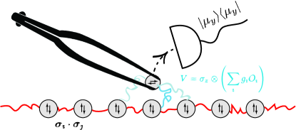
Figure 1: (Color online) Schematic of the measurement setup. A two-level ancilla interacts for a time $\tau$ with a specific site or a collection of sites in the lattice, after which a projective measurement is performed on the ancilla.

We wish to study the effect of measurements on many-body systems but, as mentioned in the introduction, solving many-body problems can be extremely difficult, and with the added complication of non-equilibrium stochastic behavior the problem is not getting any easier. We will describe how to simulate a measurement scheme in terms of matrix product states (MPS) Vidal (2004); Daley et al. (2004) or projected entangled pair states Verstraete and Cirac (2004) (PEPS) (the methods presented here can be extended very easily from the latter to the former). It will turn out that local measurements and certain global measurements have a natural description in terms of matrix product states, and since measurements are intimately connected to entanglement, this description will also highlight aspects of the entanglement properties of matrix product states.

First we will briefly review the basics of matrix product states. Any use of this technique begins with a factorization of the full many-body Hilbert space into elementary constituents of dimension $d$. This factorization is done such that the states of interest only contain a limited amount of entanglement between its subsystems (in the sense of small Schmidt-number between any bipartite cut). For spins on a periodic one-dimensional lattice of length $L$ it is natural to factor the Hilbert-space into a product of single sites. The MPS ansatz is a parametrization of the expansion coefficients in the product basis

$$\mathinner{|{\psi}\rangle}=\sum_{\sigma_{1}\ldots\sigma_{L}}\operatorname{Tr}\left(T^{[1],\sigma_{1}}T^{[2],\sigma_{2}}\ldots T^{[L],\sigma_{L}}\right)\bigotimes_{i=1}^{L}\mathinner{|{\sigma_{i}}\rangle},$$ (1)

where $T^{[i],\sigma_{i}}$ are $d$ $D\times D$ matrices (or a $d\times D\times D$ tensor), where $D$ is called the virtual dimension and $\mathinner{|{\sigma_{i}}\rangle}$ denote the $d$ single-site basis states. The trace operation in (1) is carried out over the virtual dimensions and results in coefficients of the different product states—the larger the virtual dimension $D$, the more entanglement is supported by the ansatz.

If one wishes to consider a system with open boundary conditions one can take the first and final matrices $T^{[1]}$ and $T^{[L]}$ to have dimensions $1\times D$ and $D\times 1$ respectively. The essential feature of this parametrization is that any Schmidt-decomposition of the above state will contain at most $D$ terms, thus limiting the entanglement entropy between any bipartite splitting in a systematic way. Reciprocally, it can also be shown that any state where all bipartite splittings contain at most $D$ terms are of this form Vidal (2004).

Single site reduced density-matrices for states of this form can be calculated in a clever way Verstraete et al. (2008) using only $O(Ld^{2}D^{3})$ operations. Similarly, few-site density-matrices can be calculated efficiently. Thus, expectation values of local and correlation-observables can be calculated efficiently for matrix product states.

Using variational methods it is possible not only to find good approximations for ground-states of nearest-neighbor Hamiltonians, but also Greens-functions, thermal states and time-evolution of these states, etc. Verstraete et al. (2008); Vidal (2004). All these variational methods essentially rely on the matrix element $\mathinner{\langle{\chi|A|\psi}\rangle}$ between any two matrix-product states and an operator $A$ to be calculated efficiently, which is often possible for physically relevant operators, like tensor-products of local operators.

A special set of efficiently contractible operators are the matrix product operators (MPO), which are constructed in the same way as matrix product states. An MPO is parametrized as

$$A=\sum_{j_{1},\ldots,j_{L}}\operatorname{Tr}\left(M^{[1],j_{1}}\ldots M^{[L],j_{L}}\right)\bigotimes_{i=1}^{L}X_{j_{i}},$$ (2)

where $M^{[i],j_{i}}$ are $D\times D$ matrices and the $N=d^{2}$ operators $X_{j}$ constitute a basis for the operators on a single site. If we choose the matrix-basis as the $X_{j}$ (i.e. $\mathinner{|{\sigma}\rangle}\mathinner{\langle{\sigma^{\prime}}|}$), the matrices $M^{[i],j_{i}}$ can be thought of as matrices of operators.

If $A$ is of this form, applying $A$ to $\mathinner{|{\psi}\rangle}$ in (1) amounts to the update rule $T^{\prime[j],\sigma_{j}}_{(\alpha\alpha^{\prime}),(\beta\beta^{\prime})}=\sum_{\sigma_{j}^{\prime},i_{j}}T^{[j],\sigma^{\prime}_{j}}_{\alpha\beta}M^{[j],i_{j}}_{\alpha^{\prime}\beta^{\prime}}\mathinner{\langle{\sigma_{j}|X_{i_{j}}|\sigma_{j}^{\prime}}\rangle}$, where $(\alpha\alpha^{\prime})$ is to be understood as a combined index as in the Kronecker matrix-product $C_{(ik),(jl)}=A_{ij}B_{kl}$. The virtual dimension of $A\mathinner{|{\psi}\rangle}$ will then be the product of the virtual dimensions of $A$ and $\mathinner{|{\psi}\rangle}$. In practice however, it is not desirable and often not necessary to increase the virtual dimension as one can use a variational method Verstraete et al. (2004a) to find a matrix product state $\mathinner{|{\chi}\rangle}$ of a given virtual dimension that minimizes $\left\|\mathinner{|{\chi}\rangle}-A\mathinner{|{\psi}\rangle}\right\|^{2}$. In, e.g., time-evolution, where $A$ is an approximation to the unitary time-evolution operator, one is interested in keeping a fixed virtual dimension, and the error associated with this truncation is usually negligible for short times. As shown in Hartmann et al. (2009) it is also possible to perform the time evolution in the Heisenberg picture using matrix product operators.

The above techniques can be generalized in terms of projected entangled pair states (PEPS) Verstraete and Cirac (2004), where the state is written in terms of a general tensor-network Cirac and Verstraete (2009) instead of just nearest neighbor contractions on a one-dimensional lattice. For these kinds of states it is possible to formulate variational methods in much the same way as for MPS, but the numerical stability and time-complexity of the methods can depend drastically on the topology of the graph. For an open one-dimensional lattice with nearest-neighbor interactions calculating ground states and performing time-evolution scales as $O(LD^{3})$, whereas, for a one-dimensional lattice with periodic boundary-conditions, the calculations scales as $O(LD^{5})$ due to the loop in the factorization-graph Markov and Shi (2008).

The topology of the factorization-graph is usually determined by the interactions in the system, and may be a chain, a loop, a grid, a tree or some variation of these depending on the system. Since non-local measurements can induce entanglement directly between the measured subsystems due to the obtained information, the topology can also depend on the type of measurements being performed on the system.

III The quantum theory of measurements

If we wish to simulate the stochastic evolution of a quantum system subject to measurements we can use several, closely related, techniques depending on the type of measurement being performed.

When a quantum system is being measured, the quantum state $\mathinner{|{\psi}\rangle}$ changes because the measurement alters the observers knowledge of the system. Formally this back-action is described by the action of a set of operators $\{\Omega_{\mu}\}$, where the state conditioned on the measurement outcome $\mu$ is $\Omega_{\mu}\mathinner{|{\psi}\rangle}/\sqrt{\mathinner{\langle{\psi|\Omega_{\mu}^{\dagger}\Omega_{\mu}|\psi}\rangle}}$. In general, such a set of operators is a valid measurement scheme if $\sum_{\mu}\Omega_{\mu}^{\dagger}\Omega_{\mu}=\mathds{1}$. It can be shown Nielsen and Chuang (2000) that the action of any such set of operators can be implemented by coupling the measured system unitarily to an auxiliary system and performing a projective measurement on the auxiliary system. In particular, consider a two-level ancilla interacting with the probed system. If $\sigma_{z}$ acts on the ancilla space and $A$ is an observable of the probed system with spectral resolution $A=\sum_{a}aP_{a}$ ($P_{a}$ is the projector onto the eigenspace associated with the eigenvalue $a$), then an interaction on the form

$$V=g\sigma_{z}A,$$ (3)

applied for a time $\tau$ will result in a time-evolution described by

$$U=\exp(-i\tau V)=\sum_{a}\mathcal{D}(2\phi a,\boldsymbol{z})\otimes P_{a}$$ (4)

where $\mathcal{D}$ is the spin $1/2$ rotation-operator on the ancilla-spin system and $\phi=g\tau$. In words, depending on the value of the system observable $A$, the effective spin ancilla will be rotated an angle $2\phi a$ around the $z$-axis. If we initialize the ancilla spin in state $\mathinner{|{+_{x}}\rangle}$ pointing in the $x$-direction and subsequently measure the $y$-component, we thus gain partial information about the operator $A$. Performing this measurement with the outcome $\mu=\pm 1$ for the $\sigma_{y}$-readout, corresponds to the action of the measurement operators

$$\Omega_{\mu} =(\mathinner{\langle{\mu_{y}}|}\operatorname{\otimes}\mathds{1})U(\mathinner{|{+_{x}}\rangle}\operatorname{\otimes}\mathds{1})=\frac{1}{2}\left(e^{-i\phi A}+i\mu e^{i\phi A}\right)$$ (5)

up to an arbitrary phase. Note that since we are coupling the system to a qubit-ancilla we can maximally gain one classical bit of information from the system for each measurement. Controlling $\phi$ by varying the interaction time $\tau$ or strength $g$ we can vary the strength of the measurement. For $\phi=0$ no measurement is performed. Continuous measurements with infinitesimal changes of $\mathinner{|{\psi}\rangle}$ correspond to the limit of frequent applications of weak measurements, $\phi\to 0$, while for $\phi\sim 1$ the measurement back-action becomes large.

We can use this formalism to propagate a system being measured with some rate $\kappa$ by simply evolving the state $\mathinner{|{\psi}\rangle}$ unitarily with system Hamiltonian $H$, for a time $\delta t=1/\kappa$, and then apply the measurement operator $\Omega_{\mu}$: $\mathinner{|{\psi}\rangle}\to\Omega_{\mu}\mathinner{|{\psi}\rangle}/\sqrt{p(\mu)}$, where we assume the measurement is much faster than $\delta t$ and $\mu$ is chosen randomly according to the distribution $p(\mu)=\mathinner{\langle{\psi|\Omega_{\mu}^{\dagger}\Omega_{\mu}|\psi}\rangle}$. This is then repeated until the desired final time.

If the system is continuously monitored, we model the measurement process as a limit of the above procedure in the following sense: When all the $\Omega_{\mu}$ are infinitesimally close to the identity, and the measurements are performed with a large rate compared to the system dynamics, the accumulated effect of measurements in any given time-interval (small on the timescale of unitary evolution) amounts to $N_{\mu}$ applications of $\Omega_{\mu}$ where $N_{\mu}$ are binomially distributed random numbers. Performing the limiting procedure results in a stochastic differential equation.

To be precise, if $\phi\ll 1$ and $1/\kappa\ll t_{sys}$ then the accumulated effect of $N=\kappa\Delta T$ measurements in a time $\Delta T$ is given by

$$\begin{split}\Omega(N_{+},N_{-})\propto\mathds{1}+\phi A(N_{+}-N_{-})\\ +\frac{1}{2}\phi^{2}A^{2}((N_{+}-N_{-})^{2}-2N).\end{split}$$ (6)

In the limit $N\gg 1$ we can apply the central-limit theorem to obtain $N_{+}-N_{-}\approx 2\kappa\Delta T\phi\mathinner{\langle{A}\rangle}+\sqrt{\kappa}\Delta W$, where $\Delta W$ is a normally distributed stochastic variable with zero mean and variance $\Delta T$. The accumulated effect of the measurements can then be written as

$$\begin{split}\Omega(N_{+},N_{-})\propto\mathds{1}+2\Delta T\phi^{2}\kappa\mathinner{\langle{A}\rangle}A-\frac{1}{2}\Delta T\phi^{2}\kappa A^{2}\\ +\Delta W\sqrt{\phi^{2}\kappa}A,\end{split},$$ (7)

Including the Hamiltonian evolution of the system and state-normalization, then in the limit $\Delta T\to dt$ we get the stochastic differential equation

$$\begin{split}d\mathinner{|{\psi}\rangle}=-iHdt\mathinner{|{\psi}\rangle}+dt\frac{\Gamma}{2}\left(2\mathinner{\langle{A}\rangle}A-A^{2}-\mathinner{\langle{A}\rangle}^{2}\right)\mathinner{|{\psi}\rangle}\\ +\sqrt{\Gamma}(A-\mathinner{\langle{A}\rangle})dW\mathinner{|{\psi}\rangle},\end{split}$$ (8)

where $\Gamma=\phi^{2}\kappa$ is the measurement strength.

IV Stochastic propagation of matrix product states

If we consider measurements on a system described by an MPS then we proceed as described in section III: Propagate $\mathinner{|{\psi}\rangle}$ unitarily for a time $\delta t$ and then apply $\Omega_{\mu}$ with probability $p(\mu)=\mathinner{\langle{\psi|\Omega_{\mu}^{\dagger}\Omega_{\mu}|\psi}\rangle}$. If $\Omega_{\mu}$ is efficiently contractible we can use the same variational principle as used for time-evolution, to find the matrix-product state of a given virtual dimension which best approximate $\Omega_{\mu}\mathinner{|{\psi}\rangle}$.

In particular, if $\Omega_{\mu}$ can be written as a matrix-product operator the matrix-element $\mathinner{\langle{\chi|\Omega_{\mu}|\psi}\rangle}$ for any MPS ansatz $\mathinner{|{\chi}\rangle}$ can be calculated. The probability $p(\mu)=\mathinner{\langle{\psi|\Omega_{\mu}^{\dagger}\Omega_{\mu}|\psi}\rangle}$ can also be calculated efficiently since $\Omega_{\mu}^{\dagger}\Omega_{\mu}$ is also a matrix-product operator, although possibly of a higher virtual dimension. In particular if the system is measured at a single site, $\Omega_{\mu}$ and $\Omega_{\mu}^{\dagger}\Omega_{\mu}$ are just tensor products of a number of identities and a single-site operator. In this case the application of $\Omega_{\mu}$ to the MPS is of course trivial just as the application of any local operator $V$ is trivial for an MPS: Simply update $T^{\prime[i],\sigma_{i}}_{\alpha\beta}=\sum_{\sigma_{i}^{\prime}}T^{[i],\sigma^{\prime}_{i}}_{\alpha\beta}\mathinner{\langle{\sigma_{i}|V|\sigma_{i}^{\prime}}\rangle}$, where $V$ acts on site $i$.

We thus find that many-body systems with local interactions combined with single-site measurements are easy to simulate using matrix product states in one dimension or PEPS in higher dimensions. If, however, the measurement extends across multiple sites, e.g. if our probe is not absolutely confined to a single site, then we need to decompose $\Omega_{\mu}$ into an MPO and use the variational methods in order to avoid growth of the virtual dimension of the state.

We will now consider the measurement discussed in section III described by (3), (4) and (5), but with $A$ a sum of local operators, i.e. $A=\sum_{i}g_{j}O_{j}$. This can arise either as a combined simultaneous interaction, but also as result of a sequential interaction of an ancilla with multiple sites. As in equation (5) the measurement operators for this measurement is given by

$$\Omega_{\mu} =\frac{1}{2}\left(e^{-i\phi\sum_{j}g_{j}O_{j}}+i\mu e^{i\phi\sum_{j}g_{j}O_{j}}\right)$$ (9)

$$=\frac{1}{2}\left(\bigotimes_{j}e^{-i\phi g_{j}O_{j}}+i\mu\bigotimes_{j}e^{i\phi g_{j}O_{j}}\right)$$ (10)

We see that applying this $\Omega_{\mu}$ to a general MPS results in a superposition of two MPS each a copy of the original state but multiplied with the product-operators $\otimes_{j}\exp(\pm i\phi g_{j}O_{j})$. One should think that such a superposition state would not be well represented by an MPS, but if we increase the virtual dimension of the state from $D$ to $2D$ we can in fact represent the state exactly as well as any superposition of two MPSs McCulloch (2007).

Indeed, $\Omega_{\mu}$ can be written as an MPO with tensors

$$\begin{split}M^{[1]}&=\begin{pmatrix}\frac{1}{2}\exp(-i\phi g_{1}O_{1})&\frac{1}{2}i\mu\exp(i\phi g_{1}O_{1})\end{pmatrix}\\ M^{[i]}&=\begin{pmatrix}\exp(-i\phi g_{i}O_{i})&0\\ 0&\exp(i\phi g_{i}O_{i})\end{pmatrix}\\ M^{[L]}&=\begin{pmatrix}\exp(-i\phi g_{L}O_{L})\\ \exp(i\phi g_{L}O_{L})\end{pmatrix},\end{split}$$ (11)

i.e., of virtual dimension 2. Note that it is the use of a 2-dimensional ancilla, that results in virtual dimension 2. Had we used an $n$-dimensional ancilla, generically we would need a virtual dimension of $n$ for the MPO. For the calculation of the branching probabilities $p(\mu)$, we note that also $\Omega_{\mu}^{\dagger}\Omega_{\mu}$ can be represented by an MPO of virtual dimension 3, since $\Omega_{\mu}^{\dagger}\Omega_{\mu}=\frac{1}{2}(\mathds{1}+2\mu i(\exp(2i\phi A)-\exp(-2i\phi A)))$.

As mentioned above, the variational method can now be applied to find a matrix-product state with a specified virtual dimension which is closest to $\Omega_{\mu}\mathinner{|{\psi}\rangle}$. The truncation-error for the posterior state will naturally depend not only on how close to the identity $\Omega_{\mu}$ is, but also on the state being measured. As an example, an initially uncorrelated spin-chain where all the spins point in the $x$-direction, will get long-range correlations if we, e.g., measure the $z$-component of the total spin to 0. If however, a measurement of the $x$-component is performed, the spin-chain will remain in a product state.

In the above measurement scheme the rate $\kappa$ is the inverse of the simulation time-step and the measurement strength $\phi$ can be adjusted. If we wish to model continuous measurements, the measurement rate and strength can no longer be chosen independently and the accumulated effect of many measurements for each simulation time-step has to be taken into account. One approach would be to implement the limit discussed in section III by simply choosing smaller time-steps and scaling $\phi$ accordingly. But then a larger number of truncations will be performed, so even if one is able to apply the measurement exactly the regular time-evolution may lead to an increased error.

If we seek to approximate the continuous measurement regime, the time-evolution is given by (8), which is not only non-linear in $\mathinner{|{\psi}\rangle}$ via the terms $\mathinner{\langle{A}\rangle}A$ and $\mathinner{\langle{A}\rangle}^{2}$, but also contains terms proportional to $A^{2}$, which cannot readily be cast into a matrix-product form. In each time-step, however, we can calculate $\mathinner{\langle{A}\rangle}$ and pick a random $\Delta W$ to select the relevant $\Omega$-operator. To apply this operator to $\mathinner{|{\psi}\rangle}$ we need to evaluate $\mathinner{\langle{\chi|\Omega|\psi}\rangle}$ as described in section II, but even though $\Omega$ is not on a clear MPO-form one can just evaluate the terms separately, provided $A^{2}$ is not too pathological. This amounts to the stochastic Euler method which has a global error of $O(\Delta t^{1/2})$ Kloeden and Platen (1995).

Alternatively, and in general, if the measurement extends over more than one site, it is of course always possible to combine those subsystems into a single Hilbert space and then apply the measurement operator directly on that space. If the measurement has sufficiently small support, this will not ruin the power of MPS, since it only treats a small part of the system exactly.

V Numerical examples

Figure 2: (Color online) Examples of posterior states after different types of measurement on the spin-chain ground state. In both plots $\phi=0.3\pi/4$ using the measurement operators (5). The plotted values are $\mathinner{\langle{\sigma_{z}^{i}}\rangle}$ (red) $\mathinner{\langle{\sigma_{y}^{i}}\rangle}$ (blue) and $\mathinner{\langle{\sigma_{z}^{1}\sigma_{z}^{i}}\rangle}$ for the ground state (solid black) for states subject to $\Omega_{+}(A=\sigma_{z}^{1})$ in 2a and $\Omega_{+}(A=\sigma_{z}^{1})\Omega_{+}(A=\sigma_{y}^{L})$ in 2b.

We have applied the above techniques to a spin-1/2 chain with an anti-ferromagnetic Heisenberg Hamiltonian

$$H=\frac{1}{2}J\sum_{\langle i,j\rangle}\boldsymbol{\sigma}_{i}\cdot\boldsymbol{\sigma}_{j},$$ (12)

where the sum is over nearest neighbors. We first find an MPS for the ground state, and with this as our initial state we begin to probe the system with the measurement scheme outlined above.

V.1 Local measurements

The interesting regime in this numerical study is when the measurement- and Hamiltonian dynamics are of comparable importance, but let us first imagine a projective measurement of the $z$-component spin on one of the end-points of the chain. Since the reduced density-matrix for each site in the anti-ferromagnetic ground-state are completely mixed (the Hamiltonian is rotational invariant), the expectation value of the local spin is zero and hence the projective measurement will have probability $1/2$ for both $\mathinner{|{+_{z}}\rangle}$ and $\mathinner{|{-_{z}}\rangle}$. The spin is, however, correlated with its neighbors, and the spin-expectation-value of the conditioned state $\mathinner{\langle{\sigma_{z}^{i}}\rangle}_{\mathrm{cond}}$ is directly related to the ground state correlation function.

Rewriting the correlation-function between two arbitrary spins in terms of the projector onto eigenspaces of the $i$’th spin-$z$, $P_{+/-}^{i}$, we obtain

$$\mathinner{\langle{\sigma_{z}^{i}\sigma_{z}^{j}}\rangle}=\frac{1}{2}\left(\mathinner{\langle{P_{+}^{i}\sigma_{z}^{j}}\rangle}-\mathinner{\langle{P_{-}^{i}\sigma_{z}^{j}}\rangle}\right)=\mathinner{\langle{P_{+}^{i}\sigma_{z}^{j}}\rangle}=-\mathinner{\langle{P_{-}^{i}\sigma_{z}^{j}}\rangle},$$

since the ground state is invariant under $\sigma_{z}^{j}\to-\sigma_{z}^{j}$ for all $j$. But $\mathinner{\langle{P_{\pm}\sigma_{z}^{j}}\rangle}$ is proportional to the conditioned expectation value of $\sigma_{z}^{j}$.

To get a feel for what a single measurement (close to the projective case) can do to a spin-chain ground state see figure 2. Figure 2a shows data for the state $\Omega_{+}\mathinner{|{\psi}\rangle}$, where $\Omega_{\mu}$ is given by (5) with $\phi=0.3\pi/4$ and $A=\sigma_{z}^{1}$. We see, as noted above, the spins align (on average) with the $z$-$z$ correlation function and nothing happens to the $\sigma_{y}$-average. In addition, $\mathinner{\langle{\sigma_{z}^{1}\sigma_{z}^{i}}\rangle}$ is less modulated than in the initial ground state due to the partial projection. In figure 2b we show the effects of a joint measurement, where we couple two ancillas to the system—one to $\sigma_{z}^{1}$ and one to $\sigma_{y}^{L}$. Notice how the $z$ and $y$-averages follow their respective correlation-functions from each end of the spin-chain.

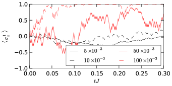
Figure 3: (Color online) Trajectories for single-site measurements with varying strengths showing both the quantum zeno- and weak-limit of the measurements. In all simulations $\kappa=100J$ and the values of $\phi$ are shown in the legend.

If the system- and measurement-dynamics occur on the same timescale the dynamics becomes far more complex. We have simulated repeated measurements over time for a spin-chain with 60 spins with varying measurement strengths $\phi$, as shown in figure 3, where time-series for $\mathinner{\langle{\sigma_{z}^{1}}\rangle}$ is shown. For weak measurements (black solid and dashed) the measurements are not strong enough to project the spin to a $\sigma_{z}$-eigenstate, since the spin is strongly driven by its neighbors. For strong measurements (red dashed) the interaction is not strong enough to drive the measured spin away from its measured value quickly enough, and we observe a quantum zeno effect on the first spin; effectively pinning the spin to a random, but definite, direction. In the intermediate regime (red solid) the measured spin exhibits oscillations with comparable signatures from both measurement- and interaction-dynamics.

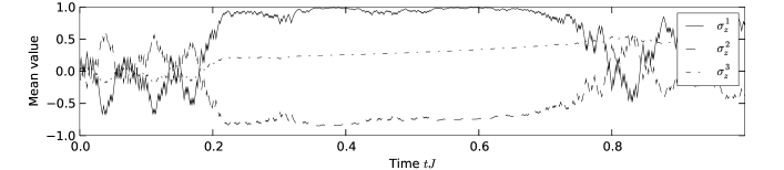
Figure 4: Time-series of $\mathinner{\langle{\sigma_{z}^{1}}\rangle}$ (solid), $\mathinner{\langle{\sigma_{z}^{2}}\rangle}$ (dashed) and $\mathinner{\langle{\sigma_{z}^{3}}\rangle}$ (dash-dotted) for measurements using (5) with $A=\sigma_{z}^{1}$ for $\phi=0.05$ and $\kappa=100J$.

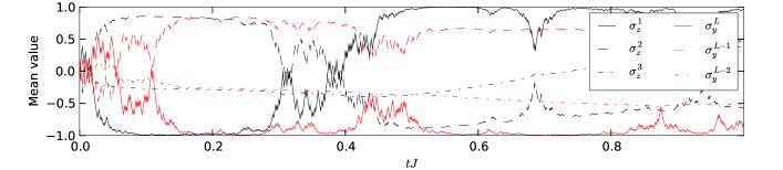
Figure 5: (Color online) Time-series for measurements using (5) with both $A=\sigma_{z}^{1}$ and $A=\sigma_{y}^{L}$ for $\phi=0.05$ and $\kappa=100J$.

In figure 4 the single-site scheme has been simulated (as in figure 2a) and the expectation-values of $\sigma_{z}$ for the first three spins are shown as function of time. As noted above the measurements induce oscillations in the average-spin values, and in the example shown, the measurements are strong enough to project the first spin onto an eigenstate for a long interval of time. Note also that the second and third spins reflect anti-correlation and correlation with the first spin respectively, both in time-intervals, when the spin is almost in a $\sigma_{z}$-eigenstate, and when $\mathinner{\langle{\sigma_{z}^{1}}\rangle}$ is close to zero.

Notice, that the anti-correlations persist even after the measured spin has been almost completely projected. This can be understood, if we consider the weak measurements as a stochastic perturbation: In order to excite the high-energy non-anti correlated eigenstates of $H$ the stochastic perturbation needs to have significant support at frequencies of comparable magnitude. Since this particular measurement is weak it does not provide enough energy to excite these states.

Figure 5 shows simulations, where $\sigma^{1}_{z}$ measurements are performed on site 1 and $\sigma_{y}^{L}$ at the end $L=60$ as in figure 2b. Here we also see the characteristic oscillations of measurements competing with interactions. In this case the measurements appear to be completely independent. In the very long time-limit, one might expect to see temporal correlations arise due to propagation-effects along the chain.

V.2 Non-local measurements

Figure 6: (Color online) To deal with non-local measurements, e.g., by sequential system-ancilla interactions (left), in the PEPS-formalism it is necessary to add an additional entanglement-bond in order to provide an efficient parametrization of the many-body state (right).

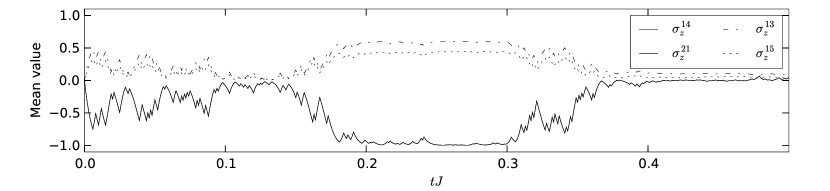
Figure 7: Time-series for a measurement using (5) for $A=\sigma_{z}^{14}+\sigma_{z}^{21}$, $\phi=0.1$ and $\kappa=100J$.

In figure 6 we consider a process where we measure two sites far from each other at the same time. This might be accomplished by an ancilla first interacting with site $i$, then with site $j$ and then being projectively measured.

This can be simulated in two ways within the theory of MPS and PEPS. One way is to keep the usual matrix product states and simply apply (9) in the form of MPO as in (11) where $g_{k}=0$ for $k\neq i,j$. The result of such a simulation can be seen in figure 7, where we have simulated a measurement of the sum $\sigma_{z}^{14}+\sigma_{z}^{21}$ in a lattice of 30 spins. In the simulation we see many of the same features as in figures 4 and 5, where the spin-expectation values are projected onto eigenstates of the observable $A$. In this case the observable $A$ also has eigenstates with eigenvalue 0, and in the simulations (figure 7) we see a projection onto this eigenvalue for $t>4$. By closer inspection of the simulation data it was found that in the periods where the measured spins have average value 0, the two-site density matrix is a slightly asymmetric statistical mixture of the $\mathinner{|{S=0,m=0}\rangle}$ and $\mathinner{|{S=1,m=0}\rangle}$ state with a purity of about $50\%$.

For sites not too far apart this works well, but truncation-error will quickly become a problem due to the emerging entanglement between site $i$ and $j$. If the sites are far apart, however, one might introduce a PEPS-graph as shown to the right in figure 6, where an extra entanglement bond has been introduced between the two distant sites. This topology constitutes a new parametrization of our states, but it is also a good illustration of the physical effects of the measurement: We are now, effectively dealing with a kind of closed boundary conditions mediated by measurements. This entails an increase in computational complexity as mentioned above, but it is still possible to use many of the same numerical tricks and techniques as used in open- and closed boundary conditions in usual MPS-simulations.

VI Conclusion and outlook

In summary we have shown how to simulate measurements on a quantum many-body system described by a MPS or PEPS formalism. In particular, a natural class of measurement-schemes can be represented simply by matrix product operators and their PEPS-equivalents. We have illustrated the use of these techniques on the anti-ferromagnetic Heisenberg spin-chain ground state and investigated the dynamics resulting from particular weak measurement schemes.

There are a number of natural applications and extensions of this work. Cold atoms in optical lattices constitute a very attractive model of many-body dynamics, where both direct optical imaging by a high aperture lens Bakr et al. (2009) and by the transmission properties of an optical cavity enclosing part of the atomic ensemble Karski et al. (2009); Takamizawa et al. (2006); Mekhov and Ritsch (2009a, b, c) is possible. High resolution achieved through non-linear atomic response Yavuz and Proite (2007); Gorshkov et al. (2008) as well as localized ionization signals, due to the impact of a scanning electron beam Wurtz et al. (2009), may be modelled by our approach.

This will allow studies of the interplay between measurement induced and interaction induced localization phenomena in such models. In a future perspective, closed feedback-loops on quantum many body systems may constitute a promising application to perform more general quantum state engineering and possibly to control phase transitions in many-body systems.

References

- Wurtz et al. (2009) P. Wurtz, T. Langen, T. Gericke, A. Koglbauer, and H. Ott, Phys. Rev. Lett. 103, 080404 (2009).
- Bakr et al. (2009) W. S. Bakr, J. I. Gillen, A. Peng, S. Foelling, and M. Greiner, arXiv:0908.0174 [cond-mat] (2009).
- Mekhov and Ritsch (2009a) I. B. Mekhov and H. Ritsch, Phys. Rev. Lett. 102, 020403 (2009a).
- Rom et al. (2006) T. Rom, T. Best, D. van Oosten, U. Schneider, S. Folling, B. Paredes, and I. Bloch, Nature 444, 733 (2006).
- Shi et al. (2006) Y. Y. Shi, L. M. Duan, and G. Vidal, Phys. Rev. A 74, 022320 (2006).
- Vidal (2008) G. Vidal, Phys. Rev. Lett. 101, 110501 (2008).
- Verstraete et al. (2004a) F. Verstraete, D. Porras, and J. I. Cirac, Phys. Rev. Lett. 93, 227205 (2004a).
- Vidal (2004) G. Vidal, Phys. Rev. Lett. 93, 040502 (2004).
- Verstraete et al. (2004b) F. Verstraete, J. J. Garcia-Ripoll, and J. I. Cirac, Phys. Rev. Lett. 93, 207204 (2004b).
- Verstraete and Cirac (2004) F. Verstraete and J. I. Cirac, arXiv:0407066 [cond-mat] (2004).
- Daley et al. (2004) A. J. Daley, C. Kollath, U. Schollwock, and G. Vidal, Journal of Statistical Mechanics: Theory and Experiment 2004, P04005 (2004).
- Matsukevich et al. (2008) D. N. Matsukevich, P. Maunz, D. L. Moehring, S. Olmschenk, and C. Monroe, Phys. Rev. Lett. 100, 150404 (2008).
- Sørensen and Mølmer (2003) A. S. Sørensen and K. Mølmer, Phys. Rev. Lett. 90, 127903 (2003).
- Raussendorf and Briegel (2001) R. Raussendorf and H. J. Briegel, Phys. Rev. Lett. 86, 5188 (2001).
- Verstraete et al. (2008) F. Verstraete, V. Murg, and J. I. Cirac, Adv. Phys. 57, 143 (2008).
- Hartmann et al. (2009) M. J. Hartmann, J. Prior, S. R. Clark, and M. B. Plenio, Phys. Rev. Lett. 102, 057202 (2009).
- Cirac and Verstraete (2009) J. I. Cirac and F. Verstraete, arXiv:0910.1130 [cond-mat] (2009).
- Markov and Shi (2008) I. L. Markov and Y. Shi, SIAM Journal on Computing 38, 963 (2008).
- Nielsen and Chuang (2000) M. A. Nielsen and I. L. Chuang, Quantum computation and quantum information (Cambridge University Press, 2000).
- McCulloch (2007) I. P. McCulloch, Journal of Statistical Mechanics: Theory and Experiment 2007, P10014 (2007).
- Kloeden and Platen (1995) P. E. Kloeden and E. Platen, Numerical solution of stochastic differential equations (Springer, 1995).
- Karski et al. (2009) M. Karski, L. Forster, J. M. Choi, W. Alt, A. Widera, and D. Meschede, Phys. Rev. Lett. 102, 053001 (2009).
- Takamizawa et al. (2006) A. Takamizawa, T. Steinmetz, R. Delhuille, T. W. Hänsch, and J. Reichel, Optics Express 14, 10976 (2006).
- Mekhov and Ritsch (2009b) I. B. Mekhov and H. Ritsch, Phys. Rev. A 80, 013604 (2009b).
- Mekhov and Ritsch (2009c) I. B. Mekhov and H. Ritsch (2009c), eprint arXiv:0911.0389 [quant-ph].
- Yavuz and Proite (2007) D. D. Yavuz and N. A. Proite, Phys. Rev. A 76, 041802(R) (2007).
- Gorshkov et al. (2008) A. V. Gorshkov, L. Jiang, M. Greiner, P. Zoller, and M. D. Lukin, Phys. Rev. Lett. 100, 093005 (2008).