Fourier Transform of the Stretched Exponential Function: Analytic Error Bounds, Double Exponential Transform, and Open-Source Implementation libkww.

Abstract

The C library libkww provides functions to compute the Kohlrausch-Williams-Watts function, i. e. the Laplace-Fourier transform of the stretched (or compressed) exponential function $\exp(-t^{\beta})$ for exponents $\beta$ between 0.1 and 1.9 with sixteen-digits accuracy. Analytic error bounds are derived for the low and high frequency series expansions. For intermediate frequencies the numeric integration is enormously accelerated by using the Ooura-Mori double exponential transformation. The source code is available from the project home page http://apps.jcns.fz-juelich.de/doku/sc/kww.

I Introduction

The C library libkww provides functions for computing the Laplace-Fourier transform of the stretched or compressed exponential function $\exp(-t^{\beta})$. It improves upon previous work DiWB85 ; ChSt91 in several respects: (1) A wider $\beta$ range is covered. (2) Results have the full accuracy of double-precision floating-point numbers. (3) The computation is very fast, thanks to two measures: (a) rigorous error bounds allow to maximally extend the low and high frequency domains where series expansions are used, and (b) the numeric integration at intermediate frequency is enormously accelerated by using a recent mathematical innovation, the Oouri-Mori double exponential transform. (4) The implementation is made available in the most portable way, namely as a C library.

Claims (1)–(3) require some explanation. Dishon et al. published tables for values of $\beta$ between 0.01 and 2 DiWB85 . However, for $\beta\lesssim 0.3$, those tables only cover an asymptotic power-law regime, which renders them practically useless. This will become clear in Sect. IV.3.

With respect to accuracy, one might argue that a numeric precision of $10^{-3}$ or $10^{-4}$ is largely sufficient for fitting spectroscopic data. However, violations of monotonicity at a level $\delta$ can trap a fit algorithm in a haphazard local minimum unless the minimum search step of the algorithm is correspondingly set to ${\cal O}(\delta)$. Since libkww returns function values with double precision, it can be smoothly integrated into existing fit routines.

With respect to speed of calculation, one might oppose that given todays computing power this is no longer a serious concern. However, the Fourier transform of the stretched exponential is often embedded in a convolution of a theoretical model with an instrumental resolution function, which in turn is embedded in a nonlinear curve fitting routine. In such a situation, accelerating the innermost loop is still advantageous.

The implementation in libkww is targeting a IEEE 754 compliant floating-point unit. Returned function values are accurate within the relative error of the double data type,

$$\delta:=2.2\cdot 10^{-16}\lesssim 2^{-52}.$$ (1)

Internally, series expansions and trapezoid sums are computed using long double variables, expecting that this translates at least to 80 bits (extended double) so that floating-point errors are not larger than

$$\epsilon:=5.5\cdot 10^{-20}\gtrsim 2^{-64}.$$ (2)

The modest signal-to-noise ratio $\delta/\epsilon$ made painstaking fine-tuning of the numeric integration unavoidable. The good side is that it will be easy to port libkww to other architectures.

This paper, after discussing typical application (Sect. II, App. A) and introducing some notation (Sect. III), describes the mathematical foundations of the implemented algorithm in full detail (Sects. IV, V, Apps. B, C). Based on this, the application programming interface and some test programs are documented (Sect. VI). Exemplary results are shown in Fig. 1.

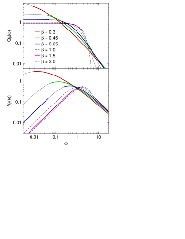
Figure 1: Fourier transforms $Q_{\beta}(\omega)$, $V_{\beta}(\omega)$ for selected values of $\beta$. Colored lines have been obtained by series expansions, solid black lines by numeric integration. Dashed lines have been computed using analytic expressions for $\beta=1,2$.

II Applications

II.1 The stretched exponential

The stretched exponential function arises in different mathematical contexts, for instance as Lévy symmetric alpha-stable distribution, or as the complement of the cumulative Weibull distribution.

In physics, the stretched exponential function is routinely employed to describe relaxation in glasses, in glass-forming liquids, and in other disordered materials. The earliest known use is by Rudolf Kohlrausch in 1854 who investigated charge relaxation in a Leiden jar. He was followed by his son Friedrich Kohlrausch in 1863 who used the stretched exponential to describe torsional relaxation in glass fibers, thereby improving previous studies by Wilhelm Weber (1841) and his father (1847). In the modern literature, these early accomplishments are often confounded, and a majority of references to Poggendorff’s Annalen der Physik und Chemie is incorrect CaCM07 .

In 1993, Böhmer et al. BoNA93 listed stretching exponents for over 70 materials, obtained by viscoelastic, calorimetric, dielectric, optical, and other linear response measurements. Other important compilations, though tinted by highly personal theoretical views, include a review by Phillips Phi96 , and a book by Ngai Nga11 . As of 2011, the Böhmer review has been cited over 1100 times, indicating a huge increase in the use of the stretched exponential function for describing relaxation phenomena. In the meantime it has also become clear that nonexpenential relaxation is not limited to supercooled, glass-forming materials but that it also occurs in in normal liquids WiWu02 ; ToBR04 ; TuWy09 .

Other physical applications of the stretched exponential function are the time dependence of luminiscence or fluorescence decays BeBV05 , and the concentration dependence of diffusion coefficients and viscosities PhPe02 . In most applications, the exponent is restricted to values $\beta\leq 1$. However, in recent years some uses of the “compressed” or “squeezed” exponential function with $1<\beta<2$ have been proposed, mostly in protein kinetics NaST04 ; FaBN06 ; HaHB06 , but also in magnetism XiFG07 .

Outside physics, the stretched exponential function has been found to provide a good fit to various socio-economic statistics, like urban agglomeration sizes, currency exchange rate variations, or the ‘success’ of scientists, musicians, and Hollywood blockbusters LaSo98 ; Dav02 ; SiRa04 .

II.2 The Kohlrausch-Williams-Watts function

The use of the Fourier transform to describe dynamic susceptibilities and scattering experiments has its foundations in linear response theory. The relations between response functions, relaxation functions, susceptibilities, correlation functions, and scattering laws are briefly summarized in Appendix A.

In 1970, Williams and Watts introduced the Fourier sine and cosine transform of the stretched exponential function to describe dielectric response as function of frequency WiWa70 . Their intuition is remarkable, since they were neither aware of earlier uses of the stretched exponential in the time domain, nor had they the technical means of actually computing the Fourier transform: based on analytic expressions for $\beta=1$ and $\beta=0.5$, they courageously extrapolated to $\beta=0.38$. In a subsequent paper WiHa71 it is quite obvious that the curves, perhaps drawn with a curving tool, are not really fits to the data.

It was noticed soon that series expansions can be used to calculate the Fourier transform of the stretched exponential in the limit of low or high frequencies WiWD71 ; LiPa80 ; MoBe84 . Based on this, computer routines were implemented that complemented these series expansions by explicit integration for intermediate frequencies DiWB85 ; ChSt91 . In actual fit routines, it was found more convenient to interpolate between tabulated values than to calculate the Fourier transform explicitely Mac97 . Other experimentalists fit their data with the Havriliak-Negami function (a Cauchy-Lorentz-Debye spectrum decorated with two fractional exponent) and use some approximations AlAC91 ; AlAC93 to express their results as Kohlrausch-Williams-Watts parameters. This clearly shows the need for an efficient implementation of the Fourier transform of the stretched exponential.

III Notation

We write the stretched exponential function in dimensionless form as

$$f_{\beta}(t):=\exp\left(-t^{\beta}\right).$$ (3)

Motivated by the relations between relaxation, linear response, and dynamic susceptibility (Appendix A), we define the Laplace-Fourier transform of $f_{\beta}$ as

$$F_{\beta}(\omega):=\int_{0}^{\infty}\!{\rm d}t\,{\rm e}^{i\omega t}\,f_{\beta}(t).$$ (4)

In most applications, one is interested in either the cosine or the sine transform,

$$\begin{array}[]{lcl}Q_{\beta}(\omega)&:=&{\rm Re}\,F_{\beta}(\omega),\\[8.61108pt] V_{\beta}(\omega)&:=&{\rm Im}\,F_{\beta}(\omega).\end{array}$$ (5)

$Q_{\beta}(\omega)$ is even in $\omega$, with

$$Q_{\beta}(0)=\Gamma(1/\beta)/\beta,$$ (6)

$V_{\beta}(\omega)$ is odd. To simplify the notation, we restrict ourselves to $\omega>0$ for the remainder of this paper.

In physical applications, the stretched exponential function is almost always used with an explicit time constant $\tau$,

$$f_{\beta,\tau}(t):=\exp\left(-(t/\tau)^{\beta}\right).$$ (7)

Its transform $F_{\beta,\tau}$ can be expressed quite simply by the dimensionless function $F_{\beta}$:

$$F_{\beta,\tau}(\omega)=\tau F_{\beta}(\tau\omega).$$ (8)

IV Series Expansions

IV.1 Small-$\omega$ expansion

For small and for large values of $\omega$, $F_{\beta}(\omega)$ can be determined from series expansions WiWD71 ; LiPa80 ; MoBe84 ; DiWB85 ; ChSt91 . For small values of $\omega$, one may expand the $\exp(i\omega t)$ term in (4). Substituting $x=t^{\beta}$, and using the defining equation of the gamma function,

$$\int_{0}^{\infty}\!{\rm d}x\,x^{\mu-1}{\rm e}^{-x}=:{\Gamma(\mu)},$$ (9)

one obtains a Taylor series in powers of $\omega$ (in Ref. MoBe84 traced back to Cauchy 1853):

$$\begin{array}[]{lcl}F_{\beta}(\omega)&=&\displaystyle\frac{1}{\beta}\sum_{k=0}^{\infty}A_{k}{(i\omega)}^{k},\\[13.77771pt] Q_{\beta}(\omega)&=&\displaystyle\frac{1}{\beta}\sum_{k=0}^{\infty}{(-1)}^{k}A_{2k}\omega^{2k},\\[13.77771pt] V_{\beta}(\omega)&=&\displaystyle\frac{1}{\beta}\sum_{k=0}^{\infty}{(-1)}^{k}A_{2k+1}\omega^{2k+1}\end{array}$$ (10)

with amplitudes

$$A_{k}=\frac{\Gamma((k+1)/\beta)}{\Gamma(k+1)}.$$ (11)

These series are useful only for small $\omega$; otherwise large alternating terms prevent efficient summation.

For $\beta\geq 1$, the series (10) converge for all values of $\omega$. For $\beta<1$, they are asymptotic expansions, which means Cop65 ; BlHa86 they diverge, but when truncated at the right place nevertheless provide useful approximations. An upper bound for the truncation error of the asymptotic series is derived in Appendix B. It is shown that the modulus of the remainder is not larger than that of the first neglected term. This improves upon a weaker and unproven estimate in Ref. ChSt91 . To minimize the truncation error, the summation must be terminated just before the term with the smallest modulus.

IV.2 Large-$\omega$ expansion

A complementary series expansion for large $\omega$ can be derived by expanding the $\exp(-t^{\beta})$ term in (4). Using

$$\int_{0}^{\infty}\!{\rm d}t\,t^{\mu-1}{\rm e}^{i\omega t}=\frac{\Gamma(\mu)}{\omega^{\mu}}{\rm e}^{i\mu\pi/2},$$ (12)

one obtains a series in powers of $\omega^{-\beta}$ (in Ref. MoBe84 attributed to Wintner 1941 Win41 ):

$$\begin{array}[]{lcl}F_{\beta}(\omega)&=&\displaystyle i\sum_{k=0}^{\infty}{(-1)}^{k}{\rm e\vphantom{()}}^{ik\beta\pi/2}B_{k}{\omega}^{-1-k\beta},\\[13.77771pt] Q_{\beta}(\omega)&=&\displaystyle\sum_{k=1}^{\infty}{(-1)}^{k-1}\sin(k\beta\pi/2)B_{k}{\omega}^{-1-k\beta},\\[13.77771pt] V_{\beta}(\omega)&=&\displaystyle\sum_{k=0}^{\infty}{(-1)}^{k}\cos(k\beta\pi/2)B_{k}{\omega}^{-1-k\beta}\\[13.77771pt] \end{array}$$ (13)

with amplitudes

$$B_{k}=\frac{\Gamma(k\beta+1)}{\Gamma(k+1)}.$$ (14)

These series are useful only for large $\omega$. Their asymptotic behavior is complementary to that of (10): For $\beta\leq 1$, they converge for all $\omega\neq 0$; for $\beta>1$, they are asymptotic expansions.

Numerically, the case $\beta\to 2$ requires special attention. The trigonometric factors in (13) can become inaccurate for large $k$ and $\beta\simeq 2$. The accuracy of $Q_{\beta}(\omega)$ can be improved if ${(-1)}^{k-1}\sin(k\beta\pi/2)$ is replaced by $\sin(k\bar{\beta}\pi/2)$ with $\bar{\beta}:=2-\beta$. Similarly, for $V_{\beta}$ we use ${(-1)}^{k}\cos(k\beta\pi/2)=\cos(k\bar{\beta}\pi/2)$.

An upper bound for the truncation error of the asymptotic series is derived in Appendix C, generalizing a result of Ref. Win41 and correcting unfounded statements of Ref. ChSt91 . If $k$ is the index of the first neglected term in (13), then the modulus of the truncation error is not larger than

$${(\sin\phi)}^{-1-k\beta}B_{k}\omega^{-k\beta+1}$$ (15)

with

$$\phi:=\left\{\begin{array}[]{ll}\pi/2&\mbox{ if }\beta\leq 1,\\[8.61108pt] \pi/(2\beta)&\mbox{ if }\beta>1.\end{array}\right.$$ (16)

IV.3 Cross-over frequencies

The leading-order terms in (10) and (13) are power-laws in $\omega$. In a plot of $\ln Q_{\beta}$ or $\ln V_{\beta}$ versus $\ln\omega$, these power-law asymptotes are straight lines that intersect at

$$\omega_{Q}:={\left(\frac{\beta\Gamma(1+\beta)\sin(\beta\pi/2)}{\Gamma(1/\beta)}\right)}^{1/(1+\beta)},$$ (17)

and

$$\omega_{V}:=\displaystyle\left(\frac{\beta}{\Gamma(2/\beta)}\right)^{1/2}.$$ (18)

For $\beta\to 0$, both cross-over frequencies go rapidly to zero, with a leading singularity

$$\omega_{Q,V}\sim\beta^{1/\beta}.$$ (19)

This explains why the limiting case $\beta\to 0$ has no practical importance, and it also explains why previously published tables DiWB85 of $Q_{\beta}(\omega)$ and $V_{\beta}(\omega)$ are useless for small exponents $\beta\lesssim 0.3$: As these tables employ the same linear $\omega$ grid for all $\beta$, for small $\beta$ they only the asymptotic large-$\omega$ power-law regime, and not the nontrivial cross-over regime for which alone a table would be needed.

For $\beta\to 2$, $\omega_{Q}$ goes to zero because of the sine term in (17) that comes from the large-$\omega$ expansion (13) of $Q_{\beta}$, as discussed above. This regime, probably of little practical importance, will be dealt with in Sect. V.5.

IV.4 Algorithm

Let as write $S$ for either $Q_{\beta}(\omega)$ or $V_{\beta}(\omega)$. We approximate $S$ by the sum (10) or (13), which we denote for short as

$$S_{n}=\sum_{k=k_{0}}^{n-1}s_{k}.$$ (20)

The return value shall have a relative accuracy of $\delta$. To avoid cancellation, the sum is computed using an extended floating-point precision $\epsilon$, as described in Sect. I. This ensures an upper bound for the total floating-point error of

$$\Delta_{\rm fp}S_{n}\leq\sum_{k=k_{0}}^{n-1}\epsilon|s_{k}|=\epsilon T_{n},$$ (21)

where we introduced the sum of absolute values

$$T_{n}:=\sum_{k=k_{0}}^{n-1}|s_{k}|$$ (22)

that needs to be computed along with $S_{n}$. An upper bound $r_{n}$ for the truncation error has been derived Appendix B or C:

$$\Delta_{\rm tr}S_{n}:=|S_{n}-S|\leq r_{n}.$$ (23)

The requested accuracy $(\Delta_{\rm fp}+\Delta_{\rm tr})S_{n}\leq\delta\cdot S_{n}$ is achieved if

$$(\epsilon T_{n}+r_{n})/S_{n}\leq\delta.$$ (24)

This leads to the following algorithm:

For each $n=k_{0}+1,k_{0}+2,\ldots$, compute $s_{n-1}$, $S_{n}$, $T_{n}$, and $r_{n}$. Terminate and return $S_{n}$ if Eq. (24) is fulfilled. Terminate and return an error code if one of the following conditions is met:

(i) $s_{k}$ is excessively large (approaching the largest floating-point number);

(ii) $s_{k}$ is excessively small (approaching the smallest normalized floating-point number);

(iii) $\epsilon T_{n}/S_{n}\geq\delta$: alternating terms have cancelled to an extent that floating-point errors may exceed $\delta$;

(iv) this is an asymptotic expansion and $r_{k+1}>r_{k}$;

(v) a preset limit $n=n_{\rm lim}$ is reached.

Since $s_{k}$ and $r_{k}$ have several common factors, involving the gamma function, these factors ought to be computed ahead to avoid the repetition of costly operations, even if this makes the loop more complicated. For $S=Q$, precomputing

$$u_{k}:=\left\{\begin{array}[]{ll}A_{2k}\omega^{2k}/\beta&\text{(small-$\omega$ expansion)},\\[8.61108pt] B_{k}\omega^{-1-k\beta}&\text{(large-$\omega$ expansion)}\end{array}\right.$$ (25)

allows to obtain quite simply

$$s_{k}=\left\{\begin{array}[]{l}(-1)^{k}u_{k},\\[8.61108pt] (-1)^{k-1}\sin(k\beta\pi/2)u_{k},\end{array}\right.$$ (26)

and

$$r_{k}=\left\{\begin{array}[]{l}u_{k},\\[8.61108pt] (\sin\phi)^{-1-k\beta}u_{k}.\end{array}\right.$$ (27)

For $S=V$, similar expressions hold. The computations for $Q$ and $V$ can be further unified by using a start index $k_{0}$ of either 0 or 1, as anticipated in Eqs. (20) to (22).

IV.5 Application domains

Let $\omega_{Q,V}^{\rm L}(\beta)$ be the smallest $\omega$ at given $\beta$ for which the small-$\omega$ algorithm returns an error code. Similarly, $\omega_{Q,V}^{\rm H}(\beta)$ is the largest $\omega$ for which the large-$\omega$ expansion fails. Fig. 2 shows these four limits, determined by a simple script (kww_findlims, cf. Sect. VI.4), as function of $\beta$. Results for $Q$ and $V$ are very similar. For $\beta<1$, the $\omega_{Q,V}^{\rm H}(\beta)$ fluctuate strongly, due to the trigonometric factor in (13).

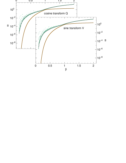
Figure 2: Frequency limits for the series expansions (10) and (13), for a required accuracy $\delta=2\cdot 10^{-16}$ and a machine precision $\epsilon=1\cdot 10^{-19}$. Orange points represent $\omega_{Q,V}^{\rm L}$, green points $\omega_{Q,V}^{\rm H}$. Black lines show the piecewise fits that are hardcoded in libkww to decide whether a series expansion is tried or whether numeric integration is used from the outset.

For later use (Sect. VI.3), the $\omega_{Q,V}^{\rm L,H}(\beta)$ are approximated by simple functions $\tilde{\omega}_{Q,V}^{\rm L,H}(\beta)$, defined piecewise after dividing the $\beta$-range $[0.1,2[$ in two or three sections. Typically, within one section, $\tilde{\omega}_{Q,V}^{\rm L,H}(\beta)$ is an exponential of a rational function with three or four parameters. Details can be found in the source kww.c where the fit results are hard-coded. For the fluctuating data at $\beta<1$, $\tilde{\omega}_{Q,V}^{\rm H}(\beta)$ approximates the lower bound rather than the full data set.

V Numeric Integration

V.1 Integrating on a double-exponential grid

Popular approaches to calculate numeric Fourier transforms include straightforward fast Fourier transform, and Tuck’s simple “Filon-trapezoidal” rule Tuc67 . Both methods evaluate the Fourier integrand on an equidistant grid $t_{k}=k\Delta t$. The Filon rule optimizes the weight of the grid points.

In our application, especially for small $\beta$, the decay of $f_{\beta}(t)$ extends over several decades. To limit the number of grid points that must be taken into account, it is customary to use a decimation algorithm. A more efficient, and perhaps even simpler alternative is the double-exponential transformation. It was first proposed by Takahasi and Mori in 1974 for the efficient evaluation of integrals with end-point singularities MoSu01 ; Mor05 . Afterwards, it was adapted to oscillatory functions by Ooura and Mori OoMo91 ; OoMo99 . The key idea is to choose grid points $t_{k}$ close to the zeros of the trigonometric function in the Fourier cosine or sine transform.

A double-exponential transformation is a monotonous function $\phi(x)$ that satisfies

$$\phi(x\to-\infty)\to 0,$$ (28)

$$\phi^{\prime}(x\to-\infty)\to 0\mbox{ double exponentially,}$$ (29)

$$\phi(x\to+\infty)\to x\mbox{ double exponentially.}$$ (30)

This transformation shall now be applied to the time variable in the Fourier integral (4):

$$t=\frac{\pi}{\omega}\phi(k-\kappa).$$ (31)

The offset

$$\kappa:=\left\{\begin{array}[]{ll}1/2&\text{ for }S=Q_{\beta}(\omega),\\[5.16663pt] 0&\text{ for }S=V_{\beta}(\omega)\end{array}\right.$$ (32)

allows us to express the cosine and the sine transform by one common equation. With the abbreviations

$$a_{k} := \pi\phi(k-\kappa),$$ (33)

$$b_{k} := \phi^{\prime}(k-\kappa)\sin(\pi(\phi(k-\kappa)+\kappa)),$$ (34)

$$\tilde{S} := \frac{\omega}{\pi}S,$$ (35)

this equation is

$$\tilde{S}=\int_{-\infty}^{\infty}\!{\rm d}k\,b_{k}f_{\beta}\left(\frac{a_{k}}{\omega}\right).$$ (36)

At this point, the integral shall be approximated by a sum, using the trapezoidal rule with stepwidth 1:

$$\tilde{S}=\sum_{k=-\infty}^{+\infty}b_{k}f_{\beta}\left(\frac{a_{k}}{\omega}\right)+\Delta_{\rm di}\tilde{S},$$ (37)

where the last term is the discretization error, to be discussed below (Sect. V.3). As a second approximation, we truncate the summation at $\pm N$,

$$\tilde{S}=\sum_{k=-N}^{+N}b_{k}f_{\beta}\left(\frac{a_{k}}{\omega}\right)+\Delta_{\rm di}\tilde{S}+\Delta_{\rm tr}\tilde{S},$$ (38)

where the new term is the truncation error, also discussed below. This sum is used in libkww to compute the KWW function at intermediate frequencies. Since $a_{k}$ and $b_{k}$ do not dependend on $\beta$ and $\omega$, they must be generated only once, which greatly accelerates repeated evaluations of (38).

In practice, (38) can be well approximated with relatively small $N$. For $k\to-\infty$, condition (29) ensures that $b_{k}$ goes double exponentially to $0$. For $k\to+\infty$, condition (30) makes the argument of the sine function in (34) tend towards $\pi k$. If $N$ is integer, then all $k$ are integer as well, and the sine can be expanded around $\sin(\pi k)=0$. In consequence, $|b_{k}|$ goes double exponentially to $0$.

V.2 Choosing a double-exponential transform

To proceed, the double-exponential transformation $\phi(k)$ must be specified. All $\phi$ considered by Ooura and Mori OoMo99 have the form

$$\phi(x)=\frac{x}{1-\exp\left(-\eta(x)\right)}.$$ (39)

Inserting this in (34), the sine term can be recast to make $b_{k}$ robust for large $k$:

$$b_{k}=\phi^{\prime}(k-\kappa)(-1)^{k}\sin\left(\frac{\pi(k-\kappa)}{{\rm e}^{\eta(k-\kappa)}-1}\right).$$ (40)

Next, the function $\eta(x)$ shall be chosen. It must fulfill the conditions

$$\eta(x\to-\infty)\to-\infty\mbox{ exponentially,}$$ (41)

$$\eta(0)=0,$$ (42)

$$\eta(x\to+\infty)\to\infty\mbox{ exponentially,}$$ (43)

Condition (42) guarantees that numerator and denominator of (39) have a zero at the same location $x=0$. This singularity is removable. To compute (38) in the case $\kappa=0$, we actually need

$$\phi(0)=\frac{1}{\eta^{\prime}(0)},\quad\phi^{\prime}(0)=\frac{1}{2}\left(1-\frac{\eta^{\prime\prime}(0)}{\eta^{\prime}(0)^{2}}\right).$$ (44)

Originally, Ooura and Mori OoMo91 had proposed

$$\eta_{\rm OM}(k):=2p\,\mbox{sinh}(hk)$$ (45)

with $p=3$ or $p=\pi$. The parameter $h$ controls the mesh width in $t$; it will be determined below (53). In a later study, Ooura and Mori suggested a more complicated function $\eta(x)$ that copes better with singularities near the real axis OoMo99 . Since our kernel $f_{\beta}(t)$ has no such singularities, we stay with the simple form (45), extending it however by a linear term that decelerates the exponential asymptote at equal $\eta^{\prime}(0)$:

$$\eta(k):=2p\,\mbox{sinh}(hk)+2qhk.$$ (46)

Given the poor signal-to-noise ratio $\delta/\epsilon$, it was not possible to find one parameterization for the entire $\beta,\omega$ domain not covered by series expansions. Therefore, distinct sets of $a_{k}$, $b_{k}$ are precomputed for five $\beta$ ranges, using the parameter set shown in Table 1.

$\beta$	$p$	$q$
0.1…0.25	1.6	0.4
0.25 …1.0	1.4	0.6
1.0 …1.75	1.0	0.2
1.75 …1.95	0.75	0.2
1.95 …2	0.15	0.4

Table 1: Hand-optimized parameters $p$, $q$ for different $\beta$ ranges, for use in the kernel $\eta$ (46) of the double-exponential transform $\phi$ (39).

V.3 Truncation error and mesh width

There are three sources of errors: Floating-point cancellation, discretization, and truncation. A bound for the floating-point error $\Delta_{\rm fp}\tilde{S}$ can be estimated as in Eq. (21). The discretization error will be controlled by iterative refinement of the grid (Sect. V.4).

Truncation errors arise from the introduction of finite summation limits in (38). The truncation error at the lower summation limit is

$$\begin{array}[]{lll}\Delta_{\rm tr}^{-}\tilde{S}&=&\displaystyle\left|\int_{-\infty}^{-N}\!{\rm d}k\,\phi^{\prime}(k)\cos(\ldots)f_{\beta}(\ldots)\right|\\[12.91663pt] &<&\displaystyle\int_{-\infty}^{-N}\!{\rm d}k\,|\phi^{\prime}(k)|.\end{array}$$ (47)

Provided $\phi^{\prime}$ does not change its sign for $k<-N$, the absolute-value operator can be omitted, and the integral becomes trivial, yielding

$$\Delta_{\rm tr}^{-}\tilde{S}<\phi(-N)<N{\rm e}^{\eta(-N)}.$$ (48)

To obtain a bound for the upper truncation error, we start from the trapezoidal sum:

$$\Delta_{\rm tr}^{+}\tilde{S}\simeq\displaystyle\left|\sum_{k=N+1}^{\infty}b_{k}f_{\beta}(\ldots)\right|$$ (49)

Using (40),

$$\Delta_{\rm tr}^{+}\tilde{S}<\displaystyle\sum_{k=N+1}^{\infty}\phi^{\prime}(k)\frac{\pi N}{{\rm e}^{\eta(k)}-1}<\displaystyle\sum_{k=N+1}^{\infty}\pi N{\rm e}^{-\eta(k)}.$$ (50)

The summands decay faster than in a geometric series so that

$$\Delta_{\rm tr}^{+}\tilde{S}<\pi N{\rm e}^{-\eta(+N)},$$ (51)

similar to (48). Altogether, the truncation error decreases double exponentially with increasing $N$. Therefore we can request at very little cost a safety factor of $m=10$ or more in the error bound,

$$\Delta_{\rm tr}\tilde{S}/\tilde{S}<\delta/m,$$ (52)

which ensures that truncation contributes almost nothing to the overall error. At this point we need a lower bound for $\tilde{S}$. From the data shown in Fig. 2, we can infer that the lowest $\tilde{S}$ that needs to be computed numerically is at $\beta=0.1$, $\omega=\omega_{V}^{\rm L}$; its value is little above $\tilde{S}_{0}:=2\cdot 10^{-20}$. The choice (46) ensures the asymptotic behavior $\eta(x)\to\pm q{\rm e}^{hx}$ for $x\to\pm\infty$. Thence (52) is satisfied by

$$h=\frac{1}{N}\ln\left(\frac{1}{q}\ln\frac{(\pi+1)mN}{\delta\tilde{S}_{0}}\right).$$ (53)

V.4 Iterative integration

The numeric integration is performed by computing the trapezoidal sum (38) in iterations $n=0,1,\ldots$ with increasing mesh size $N_{n}$ and decreasing steps $h_{n}$,

$$\tilde{S}_{n}:=\sum_{k=-N_{n}}^{N_{n}}b^{n}_{k}f_{\beta}\left(\frac{a^{n}_{k}}{\omega}\right).$$ (54)

To estimate the floating-point error, we also need the sum of absolute terms

$$\tilde{T}_{n}:=\sum_{k=-N_{n}}^{N_{n}}|b^{n}_{k}|f_{\beta}\left(\frac{a^{n}_{k}}{\omega}\right).$$ (55)

The discretization error is estimated by comparing the present with the previous result. The success criterion is

$$\Delta_{\rm fp}\tilde{S}+\Delta_{\rm di}\tilde{S}\leq\epsilon\tilde{T}_{n}+\left|\tilde{S}_{n}-\tilde{S}_{n-1}\right|\leq\delta\tilde{S}_{n}.$$ (56)

If this is fulfilled, the algorithm terminates and returns $\tilde{S}_{n}$. Otherwise, when $n$ reaches a limit $n_{\rm lim}$, the iteration exits with an error code.

In libkww, the simple iteration scheme

$$N_{n}=2^{n}N_{0}$$ (57)

is used, and $h_{n}$ is set according to (53).

V.5 Special case $\beta\to 2$

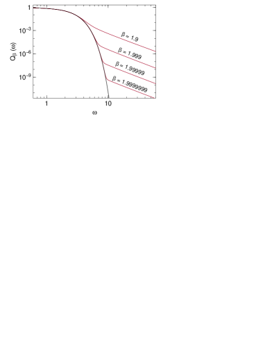
Figure 3: Red lines: Cosine transform $Q_{\beta}(\omega)$ close to the Gaussian limit $\beta\to 2$. Black line: Gaussian $\sqrt{\pi/4}\exp(-\omega^{2}/4)$.

Fig. 3 shows $Q_{\beta}(\omega)$ for representative values of $\beta$. In the limit $\beta=2$, the cosine transform is just a Gaussian,

$$Q_{2}(\omega)=\frac{\sqrt{\pi}}{2}\exp\left(-\omega^{2}/4\right),$$ (58)

whereas for $\beta\lesssim 2$ it has a power-law tail

$$Q_{2-\bar{\beta}}(\omega)\simeq\sin(\bar{\beta}\pi/2)\Gamma(2-\bar{\beta})\omega^{-3+\bar{\beta}}\mbox{ for }\omega\gg 1.$$ (59)

This qualitative change is intimately connected with the fact that the high $\omega$ expansion (13) becomes useless at $\beta=2$ where $\sin(k\beta\pi/2)=0$ for all $k$. All this is not a problem, but in the cross-over range between the two series expansions (10) and (13), the numeric quadrature fails to reach the required accuracy because of cancellation. This problem can be remediate to a certain degree by quadrating not $f_{\beta}(t)$ but the difference $f_{\beta}(t)-f_{2}(t)$. The analytic transform $Q_{2}(\omega)$ is then simply added to the numeric $\mbox{Re FT}[f_{\beta}-f_{2}]$. In our implementation, this is done for $1.75<\beta<2$. Even then, for $\beta>1.9$ the integration fails for some $\omega$.

VI Implementation

VI.1 Download and installation

Routines for the computation of $Q_{\beta}(\omega)$ and $V_{\beta}(\omega)$ have been implemented in form of a small library libkww. In order to ensure maximum portability, the programming language C has been chosen. The source code is published under the terms of the GNU General Public License (GPL); other licenses can be negotiated when needed.

The source distribution is available as a tar archiv from our institute’s application server at http://apps.jcns.fz-juelich.de/doku/sc/kww; options for long-term archival are under investigation. The build procedure is automatized with GNU autotools; the distribution contains all files needed to build the library and some test programs with the standard command sequence ./configure, make, sudo make install.

The source code resides in the subdirectory lib/. The build process normally produces a static and a dynamic version of the library libkww, and installs it to the appropriate location. Besides, a header file kww.h is copied to the appropriate include directory. Subdirectory test/ contains programs and scripts used for fine-tuning and testing.

Subdirectory doc/ provides a manual page kww (3) in plain old documentation (POD) format. The tools pod2man and pod2html are required to translate it into Unix manual ($*$roff) and HTML formats.

VI.2 Application programming interface

The application programming interface (API) can be summarized as follows:

#include <kww.h>
double  kwwc (double  omega, double  beta);
double  kwws (double  omega, double  beta);

The letters c and s stand for cosine and sine transform, respectively; the respective routines return $Q_{\beta}(\omega)$ and $V_{\beta}(\omega)$.

If $\beta$ is outside the allowed range $0.1\leq\beta\leq 2$, an error message is written to stderr, and exit is called with errno EDOM. For the cosine transform, the range $1.9<\beta<2.0$ is allowed but not supported: failures of the numeric integration in this range will not be considered bugs. If the numeric integration fails in the non-supported range, kwwc simply returns 0. Upon all other failures, an error message is written to stderr, and exit is called with errno ENOSYS.

VI.3 Algorithm

In a few special cases ($\omega=0$, or $\beta=2$ for the cosine transform), the analytically known return value is computed immediately. If $\omega<0$, the absolute value is taken; for the sine transform, a flag is set so that kwws can ultimately return $V_{\beta}(\omega)=\pm V_{\beta}(|\omega|)$ for $\omega\gtrless 0$. In the following, as everywhere else in this text, we consider only $\omega>0$.

The domain limits $\tilde{\omega}_{Q,V}^{\rm L,H}$ are implemented in functions

double kwwc_lim_low( double b );
double kwwc_lim_hig( double b );

and similar for the sine transform. If $\omega\leq\tilde{\omega}_{Q,V}^{\rm L}(\beta)$ or $\omega\geq\tilde{\omega}_{Q,V}^{\rm H}(\beta)$, the appropriate series expansion is tried. If it returns an error code (any return value below 0) which may legitimately happen for $\omega$ close to the approximate domain limit $\tilde{\omega}$, the computation falls back to the numeric integration. If $\omega$ lies between $\tilde{\omega}_{Q,V}^{\rm L}$ and $\tilde{\omega}_{Q,V}^{\rm H}$, the numeric integration is invoked from the outset.

Series expansions and numeric integration are implemented by the functions

double kwwc_low( double w, double b );
double kwwc_mid( double w, double b );
double kwwc_hig( double w, double b );

and similar for the sine transform. Since the algorithms for the cosine and sine transforms are very similar, they have a common implementation: The above functions that are actually thin wrappers around the core functions

double kww__low( double w, double b, int koffs);
double kww__mid( double w, double b, int kind);
double kww__hig( double w, double b, int koffs);

where the actual computations are carried out, following the algorithms described above (Sects. IV.4, V.4). For test purposes, all low-level functions can be called directly from outside.

VI.4 Diagnostic variables and test programs

For optimizing and testing the program it is important to know which algorithm is chosen for given $\omega,\beta$, and how many terms need to be summed. This information is provided by two global variables in the source file kww.c. Programs linked with libkww can access them using extern declarations:

extern int kww_algorithm;
extern int kww_num_of_terms;

The variable kww_algorithm is set to 1, 2, or 3, to indicate whether the low-$\omega$ expansion (10), the numeric integration (38), or the high-$\omega$ expansion (13) has been used. The variable kww_num_of_terms counts the evaluations of $f_{\beta}$.

The test program runkww (source code runkww.c in directory test/) allows to call the high-level functions of Sect. VI.2 and the low-level functions of Sect. VI.3 from the command line. If the program is called without arguments it prints a help text. Besides the function values $Q_{\beta}(\omega)$ or $V_{\beta}(\omega)$, runkww also prints the diagnostic variables described above.

The script kww_findlims.rb, written in the Ruby programming language, uses bisection to determine the limits $\omega_{Q,V}^{\rm L,H}$ where the series expansion first fails.

The program kww_countterms tests the numeric integration within a hard-coded $\beta$ range and for $\omega$ within the limits $\tilde{\omega}_{Q,V}^{\rm L,H}$, and prints the average number of evaluations of $f_{\beta}$. It has been used to optimize the parameters $p$ and $q$ of the kernel $\eta$ of the double-exponential transform $\phi$ (Sect. V.2).

The script kww_checks.rb performs scans in $\omega$ at fixed $\beta$, or vice versa, and detects points where the used algorithm or the number of function evaluations has changed. It then checks the continuity of $Q$ or $V$ across this border. Results of numerous test runs confirm that violations of monotonicity are extremely rare and never exceed a few $\delta$.

Change log

Changes to the software are described in the file CHANGE_LOG that is part of the source distribution.

Version 1 of this paper was released on arXiv (http://arxiv.org/abs/0911.4796) in 2009. Version 2 brought minor editorial changes. Version 3 was largely rewritten to describe software release kww-2.0 that provides double precision for the first time.

Appendix A Description of relaxation in time and frequency

The use of the Fourier transform to describe dynamic susceptibilities and scattering experiments has its foundations in linear response theory. In this appendix, the relations between response functions, relaxation functions, susceptibilities, correlation functions, and scattering laws shall be briefly summarized.

The linear response $B(t)$ to a perturbation $A(t)$ can be written as

$$B(t)=\int_{-\infty}^{t}\!{\rm d}t^{\prime}\,R(t-t^{\prime})\,A(t^{\prime}).$$ (60)

Consider first the momentary perturbation $A(t)=\delta(t)$. The response is $B(t)=R(t)$. Therefore, the memory kernel $R$ is identified as the response function.

Consider next a perturbation $A(t)={\rm e}^{\eta t}\Theta(-t)$ that is slowly switched on and suddenly switched off ($\Theta$ is the Heavyside step function, $\eta$ is sent to $0^{+}$ at the end of the calculation). For $t>0$, one obtains $B(t)=\Phi(t)$ where $\Phi$ is the negative primitive of the response function

$$R(t)=-\partial_{t}\Phi(t)$$ (61)

Since $\Phi$ describes the time evolution after an external perturbation has been switched off, it is called the relaxation function. Kohlrausch’s stretched exponential function is a frequently used approximation for $\Phi(t)$.

Consider finally a periodic perturbation that is switched on adiabatically, $A(t)=\exp(-i\omega t+\eta t)$, implying again the limit $\eta\to 0^{+}$. Introducing the dynamic susceptibility

$$\eta(\omega):=\int_{0}^{\infty}\!{\rm d}t\,{\rm e}^{i(\omega+i\eta)t}\,R(t),$$ (62)

the response can be written $B(t)=\eta(\omega)A(t)$. To avoid the differentiation (61) in the integrand, it is more convenient to Fourier transform the relaxation function,

$$F(\omega):=\int_{0}^{\infty}\!{\rm d}t\,{\rm e}^{i\omega t}\,\Phi(t).$$ (63)

This is Eq. (4), the starting point of the present work.

Partial integration yields a simple relation between $\eta$ and $F$:

$$\eta(\omega)=\Phi(0)+i\omega F(\omega).$$ (64)

In consequence, the imaginary part of the susceptibility, which typically describes the loss peak in a spectroscopic experiment, is given by the real part of the Fourier transform of the relaxation function, $\mbox{Im~{}}\eta=\omega\mbox{Re~{}}F(\omega)$.

Up to this point, the only physical input has been Eq. (60). To make a connection with correlation functions, more substantial input is needed. Using the full apparatus of statistical mechanics (Poisson brackets, Liouville equation, Boltzmann distribution, Yvon’s theorem), it is found Kub66 that for classical systems

$$\langle A(t)B(0)\rangle=k_{\rm B}T\Phi(t).$$ (65)

Pair correlation functions are typically measured in scattering experiments. For instance, inelastic neutron scattering at wavenumber $q$ measures the scattering law $S(q,\omega)$, which is the Fourier transform of the density correlation function,

$$S(q,\omega)=\frac{1}{2\pi}\int_{-\infty}^{\infty}\!{\rm d}t\,{\rm e}^{i\omega t}\langle\rho(q,t)^{*}\rho(q,0)\rangle.$$ (66)

In contrast to (4) and (62), this is a normal, two-sided Fourier transform. If we let $\langle\rho(q,t)^{*}\rho(q,0)\rangle=\Phi_{q}(t)$, then the scattering law $S(q,\omega)$ is

$$S(q,\omega)=\frac{1}{\pi}\mbox{Re}\;F_{q}(\omega).$$ (67)

Appendix B Truncation error in small-$\omega$ expansion

In this appendix, we derive an upper bound for the error made by truncating the small-$\omega$ expansion (10). We consider the cosine transform, and write the Taylor expansion with Lagrange remainder as

$$Q_{\beta}(\omega)=\sum_{k=0}^{n-1}Q_{\beta}^{(k)}(0)\frac{\omega^{k}}{k!}+Q_{\beta}^{(n)}(\xi)\frac{\omega^{n}}{n!}$$ (68)

with $0\leq\xi\leq\omega$. From (10), we know that

$$Q_{\beta}^{(k)}(0)=\left\{\begin{array}[]{ll}0&\mbox{ for $k$ odd,}\\[8.61108pt] \displaystyle{(-1)}^{k/2}A_{k}&\mbox{ for $k$ even.}\end{array}\right.$$ (69)

Choosing $n$ even, we have

$$\begin{array}[]{lcl}|Q_{\beta}^{(n)}(\xi)|&=&|\mbox{Re }F_{\beta}^{(n)}(\xi)|\\[8.61108pt] &\leq&|F_{\beta}^{(n)}(\xi)|\\[12.91663pt] &=&\displaystyle\left|\frac{{\rm d}^{n}}{{\rm d}\xi^{n}}\int_{0}^{\infty}\,{\rm d}t\,{\rm e}^{i\xi t}{\rm e}^{-t^{\beta}}\right|\\[12.91663pt] &=&\displaystyle\left|\int_{0}^{\infty}\,{\rm d}t\,{(it)}^{n}{\rm e}^{i\xi t}{\rm e}^{-t^{\beta}}\right|\\[12.91663pt] &\leq&\displaystyle\int_{0}^{\infty}\,{\rm d}t\,\left|{(it)}^{n}{\rm e}^{i\xi t}{\rm e}^{-t^{\beta}}\right|\\[12.91663pt] &=&\displaystyle\int_{0}^{\infty}\,{\rm d}t\,t^{n}{\rm e}^{-t^{\beta}}\\[12.91663pt] &=&\left|F_{\beta}^{(n)}(0)\right|\\[8.61108pt] &=&\left|Q_{\beta}^{(n)}(0)\right|.\end{array}$$ (70)

Therefore, the truncation error is not larger than the first neglected term. The same holds for the sine transform.

Appendix C Truncation error in large-$\omega$ expansion

In this appendix, we derive an upper bound for the error made by truncating the high-$\omega$ expansion (13). We thereby correct Ref. ChSt91 where the two incorrect statements are introduced without proof: (i) the most accurate results are obtained truncating the summation before the smallest term; and (ii) the truncation error is less than twice the first neglected term.

We specialize again to the cosine transform $Q_{\beta}(\omega)$. If we choose $\beta=4/3$ the oscillatory factor $\sin(k\beta\pi/2)$ in (13) is zero for $k=3$. If the statements of Ref. ChSt91 were correct then we could stop the summation at $k=2$ with a truncation error of zero for all values of $\omega$. This is obviously wrong. A correct truncation criterion can only be based on the amplitudes $B_{k}$; it must disregard the oscillating prefactor $\sin(k\beta\pi/2)$.

But even after omitting oscillatory factors the two statements are unfounded. In Ref. ChSt91 they are underlaid by a reference to a specific page in a book on numerical analysis Sca30 . However, that page only says “the error committed is usually less than twice the first neglected term”, followed by a reference to a specific page in a 1907 book on Celestial Mechanics Cha07 . Going back to this source, we find a rigorous theorem, which however holds only under very restrictive conditions not fulfilled here.

Figure 4: Integration path $C$ in the complex plane, used to compute an upper bound for $G^{(k)}(\xi)$.

Therefore we have to restart from scratch. We will simplify an argument of Wintner Win41 , and generalize it to cover not only the convergent case $\beta\leq 1$ but also the asymptotic expansion for $\beta>1$.

Substituting $s=\omega t$, the Fourier integral (4) takes the form

$$F_{\beta}(\omega)=\omega^{-1}\int_{0}^{\infty}\!{\rm d}s\,\exp\left(is-\omega^{-\beta}s^{\beta}\right).$$ (71)

For brevity, we discuss only the cosine transform $Q_{\beta}(\omega)=\mbox{Re }F_{\beta}(\omega)$, which we rewrite as $Q_{\beta}(\omega)=G(\omega^{-\beta})/\omega$, introducing the functions

$$G(x):=\mbox{Re}\,\int_{0}^{\infty}\!{\rm d}s\,\gamma(s,x,0)$$ (72)

and

$$\gamma(s,x,a):=s^{a}\exp\left(is-xs^{\beta}\right).$$ (73)

The Taylor expansion of $G(x)$, including the Lagrange remainder, reads

$$G(x)=\sum_{k=0}^{n-1}G^{(k)}(0)\frac{x^{k}}{k!}+G^{(n)}(\xi)\frac{x^{n}}{n!}$$ (74)

with $0\leq\xi\leq x$ and

$$G^{(k)}(\xi)={(-1)}^{k}\,\mbox{Re}\,\int_{0}^{\infty}\!{\rm d}s\,\gamma(s,\xi,k\beta).$$ (75)

Now, we choose an integration path $C$ in the complex plane, consisting of two line segments, $s$ and $s{\rm e}^{i\phi}$, and two arcs, $r{\rm e}^{i\varphi}$ and $R{\rm e}^{i\varphi}$, with $0<r\leq s\leq R<\infty$ and $0\leq\varphi\leq\phi$ as shown in Figure 4. The integral of $\gamma$ along this path is zero:

$$\int_{C}\,\!{\rm d}z\,\gamma(z,x,a)=0.$$ (76)

The contributions of the two arcs tend to 0 as $r\to 0$ and $R\to\infty$. Hence the contributions of the two line segments have equal modulus. This allows us to obtain the following bounds:

$$\begin{array}[]{lcl}\left|G^{(n)}(\xi)\right|&=&\displaystyle\left|{(-1)}^{n}\,\mbox{Re}\,\int_{0}^{\infty}\!{\rm d}s\,\gamma(s,\xi,n\beta)\right|\\[12.91663pt] &\leq&\displaystyle\left|\int_{0}^{\infty}\!{\rm d}s\,\gamma(s,\xi,n\beta)\right|\\[12.91663pt] &=&\displaystyle\left|\int_{0}^{\infty}\!{\rm d}s\,\gamma(s{\rm e}^{i\phi},\xi,n\beta)\right|\\[12.91663pt] &\leq&\displaystyle\int_{0}^{\infty}\!{\rm d}s\,\left|\gamma(s{\rm e}^{i\phi},\xi,n\beta)\right|\\[12.91663pt] &=&\displaystyle\int_{0}^{\infty}\!{\rm d}s\,\left|s^{n\beta}{\rm e}^{i\phi n\beta}\exp\left(is{\rm e}^{i\phi}-\xi s^{\beta}{\rm e}^{i\phi\beta}\right)\right|\\[12.91663pt] &=&\displaystyle\int_{0}^{\infty}\!{\rm d}s\,s^{n\beta}\exp\left(-s\sin\phi-\xi s^{\beta}\cos(\phi\beta)\right).\end{array}$$ (77)

At this point we choose

$$\phi=\left\{\begin{array}[]{ll}\pi/2&\mbox{ if }\beta\leq 1,\\[8.61108pt] \pi/(2\beta)&\mbox{ if }\beta>1,\end{array}\right.$$ (78)

which ensures $\cos(\phi\beta)\geq 0$, yielding a bound

$$\left|G^{(n)}(\xi)\right|\leq\int_{0}^{\infty}\!{\rm d}s\,s^{n\beta}\exp\left(-s\sin\phi\right)$$ (79)

that is independent of $\xi$. Evaluating the well-known integral (9) we obtain

$$\left|G^{(n)}(\xi)\right|\leq\frac{\Gamma(n\beta+1)}{{(\sin\phi)}^{n\beta+1}}.$$ (80)

Only trivial changes are needed to adapt this argument to the sin trafo $V_{\beta}(\omega)$.

References

- (1) M. Dishon, G. H. Weiss and J. T. Bendler, J. Res. N. B. S. 90, 27 (1985).
- (2) S. H. Chung and J. R. Stevens, Am. J. Phys. 59, 1024 (1991).
- (3) M. Cardona, R. V. Chamberlin and W. Marx, Ann. Phys. (Leipzig) 16, 842 (2007).
- (4) R. Böhmer, K. L. Ngai, C. A. Angell and D. J. Plazek, J. Chem. Phys. 99, 4201 (1993).
- (5) J. C. Phillips, Phys. Rev. E 53, 1732 (1996).
- (6) K. L. Ngai, Relaxation and Diffusion in Complex Systems, Springer: New York (2011).
- (7) S. Wiebel and J. Wuttke, New J. Phys. 4, 56 (2002).
- (8) R. Torre, P. Bartolini and R. Righini, Nature 428, 296 (2004).
- (9) D. A. Turton and K. Wynne, J. Chem. Phys. 131, 201101 (2009).
- (10) M. N. Berberan-Santos, E. N. Bodunov and B. Valeur, Chem. Phys. 315, 171 (2005).
- (11) G. D. J. Phillies and P. Peczak, Macromolecules 21, 214 (2002).
- (12) H. K. Nakamura, M. Sasai and M. Takano, Chem. Phys. 307, 259 (2004).
- (13) P. Falus, M. A. Borthwick, S. Narayanan, A. R. Sandy and S. G. J. Mochrie, Phys. Rev. Lett. 97, 066102 (2006).
- (14) P. Hamm, J. Helbing and J. Bredenbeck, Chem. Phys. 323, 54 (2006).
- (15) H. Xi, S. Franzen, J. I. Guzman and S. Mao, J. Magn. Magn. Mat. 319, 60 (2007).
- (16) J. Laherrère and D. Sournette, Eur. Phys. J. B 2, 525 (1998).
- (17) J. A. Davies, Eur. Phys. J. B 27, 445 (2002).
- (18) S. Sinha and S. Raghavendra, Eur. Phys. J. B 42, 293 (2004).
- (19) G. Williams and D. C. Watts, Trans. Faraday Soc. 66, 80 (1970).
- (20) G. Williams and P. J. Hains, Chem. Phys. Lett. 10, 585 (1971).
- (21) G. Williams, D. C. Watts, S. B. Dev and A. M. North, Trans. Faraday Soc. 67, 1323 (1971).
- (22) C. P. Lindsey and G. D. Patterson, J. Chem. Phys. 73, 3348 (1980).
- (23) E. W. Montroll and J. T. Bendler, J. Stat. Phys. 34, 129 (1984).
- (24) J. R. Macdonald, J. Non-Cryst. Solids 212, 95 (1997).
- (25) F. Alvarez, A. Alegría and J. Colmenero, Phys. Rev. B 44, 7306 (1991).
- (26) F. Alvarez, A. Alegría and J. Colmenero, Phys. Rev. B 47, 125 (1993).
- (27) E. T. Copson, Asymptotic Expansions, Cambridge University Press: Cambridge (1965).
- (28) N. Bleistein and R. A. Handelsman, Asymptotic Expansion of Integrals, Dover Publications: London (1986).
- (29) A. Wintner, Duke Math. J. 8, 678 (1941).
- (30) E. O. Tuck, Math. Comput. 21, 239 (1967).
- (31) M. Mori and M. Sugihara, J. Comp. Appl. Math. 127, 287 (2001).
- (32) M. Mori, Publ. RIMS, Kyoto Univ. 41, 897 (2005).
- (33) T. Ooura and M. Mori, J. Comp. Appl. Math. 38, 353 (1991).
- (34) T. Ooura and M. Mori, J. Comp. Appl. Math. 112, 229 (1999).
- (35) R. Kubo, Rep. Progr. Phys. 29, 255 (196).
- (36) J. B. Scarborough, Numerical mathematical analysis, John Hopkins Press: Baltimore (1930). The statement about usual truncation errors in asymptotic series is on p. 158 of the 2nd edition (1950), and on p. 164 of the 5th edition (1962).
- (37) C. L. Charlier, Die Mechanik des Himmels. Zweiter Band, Veit & Comp.: Leipzig (1907).