Dark Matter Particle Spectroscopy at the LHC:
Generalizing to Asymmetric Event Topologies
Abstract:
We consider SUSY-like missing energy events at hadron colliders and critically examine the common assumption that the missing energy is the result of two identical missing particles. In order to experimentally test this hypothesis, we generalize the subsystem variable to the case of asymmetric event topologies, where the two SUSY decay chains terminate in different “children” particles. In this more general approach, the endpoint of the distribution now gives the mass of the parent particles as a function of two input children masses and . We propose two methods for an independent determination of the individual children masses and . First, in the presence of upstream transverse momentum the corresponding function is independent of at precisely the right values of the children masses. Second, the previously discussed “kink” is now generalized to a “ridge” on the 2-dimensional surface . As we show in several examples, quite often there is a special point along that ridge which marks the true values of the children masses. Our results allow collider experiments to probe a multi-component dark matter sector directly and without any theoretical prejudice.
1 Introduction
A general expectation in high energy physics today is that physics beyond the standard model (BSM) should emerge at the TeV scale in order to stabilize the hierarchy between the Planck and electroweak scales. Further evidence in support of this belief is provided by the dark matter problem of astro-particle physics, which can be quite naturally solved by postulating the existence of a new, weakly-interacting dark matter particle with a mass in the TeV range. Such dark matter particles are naturally present in the most popular BSM scenarios such as supersymmetry [1], extra dimensions [2, 3, 4], little Higgs theory [5, 6] etc. They will be produced in the upcoming high-energy collisions at the Large Hadron Collider (LHC) at CERN, which offers an exciting opportunity to study dark matter in a high-energy lab. Since the dark matter particles are weakly interacting, they do not leave any deposits inside the detector and can only manifest themselves in the form of missing energy. Recently, there has been a lot of theoretical effort directed at testing the dark matter hypothesis at the LHC [7, 8, 9, 10, 11, 12, 13, 14, 15, 16] and the future International Linear Collider (ILC) [7, 17, 9, 10, 11, 18, 19, 20]. Unfortunately, most of these studies have been performed in some very model-dependent as well as very complex setup111Some notable exceptions are the studies in Refs. [7, 8].. In the literature, a typical collider study of dark matter most often starts with the assumption of a specific model with a dark matter candidate (usually supersymmetry with its myriad of parameters) and then investigates the model’s predictions for the expected rates at the LHC in one or several missing energy channels. Rarely, if ever, has the question been posed in reverse: what does the observation of a missing energy signal at the LHC tell us about the dark matter particle and its properties in a generic and model-independent way [21].
1.1 Probing the dark matter sector at colliders
Naturally, the most pertinent question after the discovery of any BSM missing energy signal at the LHC is simply whether the new signal is indeed due to the production of new massive particles, or whether it is just an enhancement in the production of SM neutrinos [21]. In principle, there are two handles that can be used in addressing this question. In order to prove dark matter production, one can measure the mass of the missing particle and show that it is different (heavier) from the SM neutrino masses. Alternatively, one can try to measure the spin of the missing particle and show that it is different from (the spin of the neutrino). While there is a large body of recent work on spin measurements in missing energy events [22, 23, 24, 25, 26, 27, 28, 29, 30, 31, 32, 33, 34, 35, 36, 37, 38, 39, 40, 41, 42, 43, 44, 45, 46, 47, 48], once again very few of those methods are model-independent [45, 47]. Furthermore, in all considered examples in the literature the spin measurement appears to be very difficult. Therefore, in this paper we shall concentrate on the question of measuring the mass(es) of the particles responsible for the missing energy. In doing so, we are motivated by two reasons. First, previous experience indicates that the mass question will be answered long before any spin measurements, and second, many of the spin determination methods require prior knowledge of the mass spectrum anyway.
The difficulty in measuring the mass of the dark matter particle at a hadron collider like the Tevatron or the LHC is widely appreciated and has generated a lot of recent activity [49, 50, 51, 52, 53, 54, 55, 56, 57, 58, 59, 60, 61, 62, 63, 64, 65, 66, 67, 68, 69, 70, 71, 72, 73, 74, 75, 76, 77, 78, 79, 80, 81, 82, 83, 84, 85, 86, 87, 88, 89, 90, 91, 92, 93, 94, 95, 96, 97, 98, 99, 100, 101, 102]. The main problem can be understood as follows. In a typical BSM dark matter scenario, the cosmological longevity of the dark matter particle is ensured by some new symmetry222Some popular examples are: -parity in supersymmetry, KK parity in Universal Extra Dimensions, -parity in Little Higgs models, -parity in warped extra dimensions, -parity in extended gauge theories, etc. under which the SM particles are singlets. At the same time, there are additional particles in the spectrum which are charged under the new symmetry. If the lightest one among those is electrically and color neutral, it is a potential dark matter candidate, whose lifetime is protected by the new symmetry. With any such setup, it is clear that single production of dark matter particles at colliders is forbidden by the symmetry. Therefore, each event has at least two missing particles, whose energies and momenta are unknown. As a rule, it is typically impossible to fully reconstruct the kinematics of such events and observe the mass of the missing particle directly as an invariant mass peak333For studies attempting full event reconstruction in long cascade chains, see Refs. [63, 75, 88, 92, 101].. Consequently, one has to resort to various indirect methods of extracting the mass of the dark matter particle.
Unfortunately, all existing studies in the literature have explicitly or implicitly made the following two assumptions:
-
•
Single dark matter component. A common assumption throughout the collider phenomenology literature is that colliders are probing only one dark matter species at a time, i.e. that the missing energy signal at colliders is due to the production of one and only one type of dark matter particles. Of course, there is no astrophysical evidence that the dark matter is made up of a single particle species: it may very well be that the dark matter world has a rich structure, just like ours [103]. Consequently, if there exist several types of dark matter particles, each contributing some fraction to the total relic density, a priori there is no reason why they cannot all be produced in high energy collisions. Theoretical models with multiple dark matter candidates have also been proposed [104, 105, 106, 107, 108, 109, 110, 111, 112].
-
•
Identical missing particles in each event. A separate assumption, common to most previous studies, is that the two missing particles in each event are identical. This assumption could in principle be violated as well, even if the single dark matter component hypothesis is true. The point is that one of the missing particles in the event may not be a dark matter particle, but simply some heavier cousin which decays invisibly. An invisibly decaying heavy neutralino ( with ) and an invisibly decaying sneutrino () are two such examples from supersymmetry. As far as the event kinematics is concerned, the mass of the heavier cousin is a relevant parameter and approximating it with the mass of the dark matter particle will simply give nonsensical results. Another relevant example is provided by models in which the SUSY cascade may terminate in any one of several light neutral particles [113].
Given our utter ignorance about the structure of the dark matter sector, in this paper we set out to develop the necessary formalism for carrying out missing energy studies at hadron colliders in a very general and model-independent way, without relying on any assumptions about the nature of the missing particles. In particular, we shall not assume that the two missing particles in each event are the same. We shall also allow for the simultaneous production of several dark matter species, or alternatively, for the production of a dark matter candidate in association with a heavier, invisibly decaying particle. Under these very general circumstances, we shall try to develop a method for measuring the individual masses of all relevant particles - the various missing particles which are responsible for the missing energy, as well as their parents which were originally produced in the event.
1.2 Generalizing to asymmetric event topologies
In general, by now there is a wide variety of techniques available for mass measurements in SUSY-like missing energy events. Such events are characterized by the pair production of two new particles, each of which undergoes a sequence of cascade decays ending up in a particle which is invisible in the detector. Each technique has its own advantages and disadvantages444For a comparative review of the three main techniques, see [85].. For our purposes, we chose to revamp the method of the Cambridge variable [50] and adapt it to the more general case of an asymmetric event topology shown in Fig. 1.
Consider the inclusive production of two identical555In principle, the assumption of identical parents can also be relaxed, by a suitable generalization of the variable, in which the mass ratio of the two parents is treated as an additional input parameter [96]. parents of mass as shown in Fig. 1. The parent particles may be accompanied by any number of “upstream” objects, such as jets from initial state radiation [66, 67, 79], or visible decay products of even heavier (grandparent) particles [85]. The exact origin and nature of the upstream objects will be of no particular importance to us, and the only information about them that we shall use will be their total transverse momentum . In turn, each parent particle initiates a decay chain (shown in red) which produces a certain number of Standard Model (SM) particles (shown in gray) and an intermediate “child” particle of mass . Throughout this paper we shall use the index to classify various objects as belonging to the upper () or lower () branch in Fig. 1. The child particle may or may not be a dark matter candidate: in general, it may decay further as shown by the dashed lines in Fig. 1. We shall apply the “subsystem” concept [77, 85] to the subsystem within the blue rectangular frame. The SM particles from each branch within the subsystem form a composite particle of known666We assume that there are no neutrinos among the SM decay products in each branch. transverse momentum and invariant mass . Since the children masses and are a priori unknown, the subsystem will be defined in terms of two “test” masses and . In Fig. 1, are the trial transverse momenta of the two children. The individual momenta are also a priori unknown, but they are constrained by transverse momentum conservation:
| (1) |
Given this very general setup, in Section 3 we shall consider a generalization777The possibility of applying the variable to an event topology with different children was previously mentioned in Refs. [95, 96]. of the usual variable which can apply to the asymmetric event topology of Fig. 1. There will be two different aspects of the asymmetry:
-
•
First and foremost, we shall avoid the common assumption that the two children have the same mass. This will be important for two reasons. On the one hand, it will allow us to study events in which there are indeed two different types of missing particles. We shall give several such examples in the subsequent sections. More importantly, the endpoint of the asymmetric variable will allow us to measure the two children masses separately. Therefore, even when the events contain identical missing particles, as is usually assumed throughout the literature, one would be able to establish this fact experimentally from the data, instead of relying on an ad hoc theoretical assumption.
-
•
As can be seen from Fig. 1, in general, the number as well as the types of SM decay products in each branch may be different as well. Once we allow for the children to be different, and given the fact that we start from identical parents, the two branches of the subsystem will naturally involve different sets of SM particles.
In what follows, when referring to the more general variable defined in Section 3, we shall interchangeably use the terms “asymmetric” or “generalized” . In contrast, we shall use the term “symmetric” when referring to the more conventional definition with identical children.
The traditional approach assumes that the children have a common test mass and then proceeds to find one functional relation between the true child mass and the true parent mass as follows [50]. Construct several distributions for different input values of the test children mass and then read off their upper kinematic endpoints . These endpoint measurements are then interpreted as an output parent mass , which is a function of the input test mass :
| (2) |
The importance of this functional relation is that it is automatically satisfied for the true values and of the parent and child masses:
| (3) |
In other words, if we could somehow guess the correct value of the child mass, the function (2) will provide the correct value of the parent mass. However, since the true child mass is a priori unknown, the individual masses and still remain undetermined and must be extracted by some other means.
At this point, it may seem that by considering the asymmetric variable with non-identical children particles, we have regressed to some extent. Indeed, we are introducing an additional degree of freedom in eq. (2), which now reads
| (4) |
The standard endpoint method will still allow us to find the parent mass , but now it is a function of two input parameters and which are completely unknown. Of course, if one knew the correct values of the two children masses and entering eq. (4), the true parent mass will be given in a manner analogous to eq. (3):
| (5) |
Our main result in this paper is that in spite of the apparent remaining arbitrariness in eq. (4), one can nevertheless uniquely determine all three masses , and , just by studying the behavior of the measured function . More importantly, this determination can actually be done in two different ways! Our first method is simply a generalization of the observation made in Refs. [65, 66, 67, 68, 85] that under certain circumstances (varying or nonvanishing upstream momentum ), the function (2) develops a “kink” precisely at the correct value of the child mass:
| (6) |
In other words, the function (2) is continuous, but not differentiable at the point . In the asymmetric case, we find that the function (4) is similarly non-differentiable at a set of points , so that the kink of eq. (6) is generalized to a “ridge” on the 2-dimensional hypersurface defined by (4) in the three-dimensional parameter space of . 888Ref. [96] studied the orthogonal scenario of different parents () and identical children () and found a similar non-differentiable feature, called a “crease”, on the corresponding two-dimensional hypersurface within the three-dimensional parameter space . Interestingly enough, the ridge often (albeit not always) exhibits a special point which marks the exact location of the true values .
Our second method for determining the two children masses and is even more general and is applicable under any circumstances. The main starting point is that just like the endpoint of the symmetric , the endpoint of the asymmetric also depends on the value of the upstream transverse momentum , so that eq. (4) is more properly written as
| (7) |
Now we can explore the dependence in (7) and note that it is absent for precisely the right values of and :
| (8) |
While this property has been known, it was rarely used in the case of the symmetric , since it offers redundant information: once the correct child mass is found through the kink (6), the parent mass is given by (2) and there are no remaining unknowns, thus there is no need to further investigate the dependence. In the case of the asymmetric , however, we start with one additional unknown parameter, which cannot always be determined from the “ridge” information alone. Therefore, in order to pin down the complete spectrum, we are forced to make use of (8). The nice feature of the method is that it always allows us to determine both children masses and , without relying on the “ridge” information at all. In this sense, our two methods are complementary and each can be used to cross-check the results obtained by the other.
The paper is organized as follows999Readers who are unfamiliar with the concept may benefit from consulting Refs. [54, 68, 85, 96] first.. In Sec. 2 we begin with a review of the conventional symmetric variable and its properties. Then in Sec. 3 we introduce the asymmetric variable and highlight its properties which are relevant for our mass measurements. We also discuss some experimental subtleties in the construction of the asymmetric distribution, which are not present in the case of the symmetric . Sections 4, 5.1 and 5.2 present some simple examples of asymmetric event topologies. Finally, Sec. 6 summarizes our main results and outlines some possible directions for future work. Appendix A revisits the examples of Section 4 in the case of , which can be handled by purely analytical means [96].
2 The conventional symmetric
2.1 Definition
We begin our discussion by revisiting the conventional definition of the symmetric variable with identical daughters, following the general notation introduced in Fig. 1. Let us consider the inclusive production of two parent particles with common mass . Each parent initiates a decay chain producing a certain number of SM particles. In this section we assume that the two chains terminate in children particles of the same mass: . (From Section 3 on we shall remove this assumption.) In most applications of in the literature, the children particles are identified with the very last particles in the decay chains, i.e. the dark matter candidates. However, the symmetric can also be usefully applied to a subsystem of the original event topology, where the children are some other pair of (identical) particles appearing further up the decay chain [77, 85]. The variable is defined in terms of the measured invariant mass and transverse momentum of the visible particles on each side (see Fig. 1). With the assumption of identical children, the transverse mass of each parent is
| (9) |
where is the common test mass for the children, which is an input to the calculation, while is the unknown transverse momentum of the child particle in the -th chain. In eq. (9) we have also introduced shorthand notation for the transverse energy of the composite particle made from the visible SM particles in the -th chain
| (10) |
and for the transverse energy of the corresponding child particle in the -th chain
| (11) |
2.2 Computation
The standard definition (12) of the variable is sufficient to compute the value of numerically, given a set of input values for its arguments. The right-hand side of eq. (12) represents a simple minimization problem in two variables, which can be easily handled by a computer. In fact, there are publicly available computer codes for computing [114, 115]. The public codes have even been optimized for speed [84] and give results consistent with each other (as well as with our own code)101010Unfortunately, the assumption of identical children is hardwired in the public codes and they cannot be used to calculate the asymmetric introduced below in Section 3 without additional hacking. We shall return to this point in Section 3.. Nevertheless, it is useful to have an analytical formula for calculating the event-by-event for several reasons. First, an analytical formula is extremely valuable when it comes to understanding the properties and behavior of complex mathematical functions like (12). Second, computing from a formula will be faster than any numerical scanning algorithm. The computing speed becomes an issue especially when one considers variations of like , where in addition one needs to scan over all possible partitions of the visible objects into two decay chains [64]. Therefore, in this paper we shall pay special attention to the availability of analytical formulas and we shall quote such formulas whenever they are available.
In the symmetric case with identical children, an analytical formula for the event-by-event exists only in the special case . It was derived in [64] and we provide it here for completeness. (In the next section we shall present its generalization for the asymmetric case of different children.) The symmetric is known to have two types of solutions: “balanced” and “unbalanced” [54, 64]. The balanced solution is achieved when the minimization procedure in eq. (12) selects a momentum configuration for in which the transverse masses of the two parents are the same: . In that case, typically neither nor is at its global (unconstrained) minimum. In what follows, we shall use a superscript to refer to such balanced-type solutions. The formula for the balanced solution of the symmetric variable is given by [64, 68]
| (13) |
where is a convenient shorthand notation introduced in [68]
| (14) |
and was already defined in eq. (10).
On the other hand, unbalanced solutions arise when one of the two parent transverse masses ( or , as the case may be) is at its global (unconstrained) minimum. Denoting the two unbalanced solutions with a superscript , we have [54]
| (15) | |||||
| (16) |
Given the three possible options for , eqs. (13), (15) and (16), it remains to specify which one actually takes place for a given set of values for , , , , and in the event111111Recall that (13) only applies for .. The balanced solution (13) applies when the following two conditions are simultaneously satisfied:
| (17) | |||||
| (18) |
where
| (19) |
gives the global (unconstrained) minimum of the corresponding parent transverse mass . The unbalanced solution applies when the condition (17) is false and condition (18) is true, while the unbalanced solution applies when the condition (17) is true and condition (18) is false. It is easy to see that conditions (17) and (18) cannot be simultaneously violated, so these three cases exhaust all possibilities.
2.3 Properties
Given its definition (12), one can readily form and study the differential distribution. Although its shape in general does carry some information about the underlying process, it has become customary to focus on the upper endpoint , which is simply the maximum value of found in the event sample:
| (20) |
Notice that in the process of maximizing over all events, the dependence on , , and disappears, and depends only on two input parameters: and , the latter entering through in the momentum conservation constraint (1). The measured function (20) is the starting point of any -based mass determination analysis. We shall now review its three basic properties which make it suitable for such studies [100].
2.3.1 Property I: Knowledge of as a function of
This property was already identified in the original papers and served as the main motivation for introducing the variable in the first place [50, 54]. Mathematically it can be expressed as
| (21) |
This is the same as eq. (2), but now we have been careful to include the explicit dependence on , which will be important in our subsequent discussion. As indicated in eq. (21), the function can be experimentally measured from the endpoint (20). The crucial point now is that the relation (21) is satisfied by the true values and of the parent and child mass, correspondingly:
| (22) |
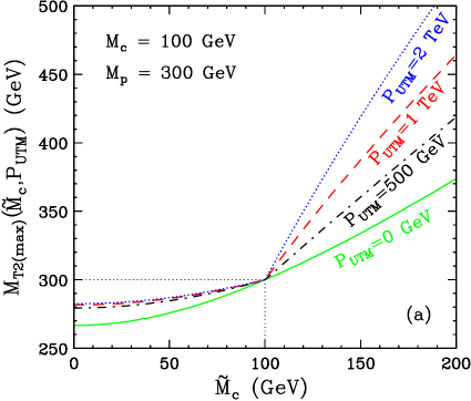
Notice that eq. (22) holds for any value of , so in practical applications of this method one could choose the most populated bin to reduce the statistical error. On the other hand, since a priori we do not know the true mass of the missing particle, eq. (22) gives only one relation between the masses of the mother and the child. This is illustrated in Fig. 2(a), where we consider the simple example of direct slepton pair production121212The corresponding event topology is shown in Fig. 3(a) below with ., where each slepton () decays to the lightest neutralino () by emitting a single lepton : . Here the slepton is the parent and the neutralino is the child. Their masses were chosen to be GeV and GeV, correspondingly, as indicated with the black dotted lines in Fig. 2(a). In this example, the upstream transverse momentum is provided by jets from initial state radiation. In Fig. 2(a) we plot the function (21) versus , for several fixed values of . The green solid line represents the case of no upstream momentum . In agreement with eq. (22), this line passes through the point corresponding to the true values of the mass parameters. Notice that the property (22) continues to hold for other values of . Fig. 2(a) shows three more cases: GeV (dotdashed black line), TeV (dashed red line) and TeV (dotted blue line). All those curves still pass through the point with the correct values of the masses, illustrating the robustness of the property (22) with respect to variations in .
2.3.2 Property II: Kink in at the true
The second important property of the variable was identified rather recently [68, 66, 65, 67, 85]. Interestingly, the endpoint , when considered as a function of the unknown input test mass , often develops a kink (6) at precisely the correct value of the child mass. The appearance of the kink is a rather general phenomenon and occurs under various circumstances. It was originally noticed in event topologies with composite visible particles, whose invariant mass is a variable parameter [68, 65]. Later it was realised that a kink also occurs in the presence of non-zero upstream momentum [66, 67, 85], as in the example of Fig. 2(a), where arises due to initial state radiation. As can be seen in the figure, the kink is absent for , but as soon as there is some non-vanishing , the kink becomes readily apparent. As expected, the kink location (marked by the vertical dotted line) is at the true child mass ( GeV), where the corresponding value of (marked by the horizontal dotted line) is at the true parent mass ( GeV). Fig. 2(a) also demonstrates that with the increase in , the kink becomes more pronounced, thus the most favorable situations for the observation of the kink are cases with large , e.g. when the upstream momentum is due to the decays of heavier (grandparent) particles [85].
2.3.3 Property III: invariance of at the true
This property is the one which has been least emphasized in the literature. Notice that the endpoint function (21) in general depends on the value of . However, the first property (22) implies that the dependence disappears at the correct value of the child mass:
| (23) |
In order to quantify this feature, let us define the function
| (24) |
which measures the shift of the endpoint due to variations in . The function can be measured experimentally: the first term on the right-hand side of (24) is simply the endpoint observed in a subsample of events with a given (preferably the most common) value of , while the second term on the right-hand side of (24) contains the endpoint of the 1-dimensional variable introduced in [100]:
| (25) |
Given the definition (24), the third property (23) can be rewritten as
| (26) |
where the equality holds only for :
| (27) |
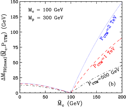
Eqs. (26) and (27) provide an alternative way to determine the true child mass : simply find the value of which minimizes the function . This procedure is illustrated in Fig. 2(b), where we revisit the slepton pair production example of Fig. 2(a) and plot the function defined in (24) versus the test mass , for the same set of (fixed) values of . Clearly, the zero of the function (24) occurs at the true child mass GeV, in agreement with eq. (27). In our studies of the asymmetric case in the next sections, we shall find that the third property (27) is extremely important, since it will always allow us the complete determination of the mass spectrum, including both children masses and .
3 The generalized asymmetric
After this short review of the basic properties of the conventional symmetric variable (12), we now turn our attention to the less trivial case of . Following the logic of Sec. 2, in Sec. 3.1 we first introduce the asymmetric variable and then in Secs. 3.2 and 3.3 we discuss its computation and mathematical properties, correspondingly.
3.1 Definition
The generalization of the usual definition (12) to the asymmetric case of is straightforward [96]. We continue to follow the conventions and notation of Fig. 1, but now we simply avoid the assumption that the children masses are equal, and we let each one be an independent input parameter . Without loss of generality, in what follows we assume . The transverse mass of each parent (9) is now a function of the corresponding child mass :
| (28) |
where the transverse energy of the composite SM particle on the -th side of the event was already defined in (10), while the transverse energy of the child is now generalized from (11) to
| (29) |
The event-by-event asymmetric variable is defined in analogy to (12) and is given by [96]
| (30) |
which is now a function of two input test children masses and . In the special case of , the asymmetric variable defined in (30) reduces to the conventional symmetric variable (12).
3.2 Computation
In this subsection we generalize the discussion in Section 2.2 and present an analytical formula for computing the event-by-event asymmetric variable (30). Just like the formula (13) for the symmetric case, our formula will hold only in the special case of . As before, the asymmetric variable has two types of solutions – balanced and unbalanced. The balanced solution occurs when the following two conditions are simultaneously satisfied (compare to the analogous conditions (17) and (18) for the symmetric case)
| (31) | |||
| (32) |
where, in analogy to (19),
| (33) |
is the test child momentum at the global unconstrained minimum of . The balanced solution for is now given by
| (34) |
where was defined in (14). For convenience, in (34) we have introduced two alternative mass parameters
| (35) | |||||
| (36) |
in place of the original trial masses and . The new parameters and are simply a different parametrization of the two degrees of freedom corresponding to the unknown child masses and entering the definition of the asymmetric . The parameters and allow us to write formula (34) in a more compact form. More importantly, they also allow to make easy contact with the known results from Section 2 by taking the symmetric limit as
| (37) |
It is easy to see that in the symmetric limit (37) our balanced solution (34) for the asymmetric reduces to the known result (13) for the symmetric .
An interesting feature of the asymmetric balanced solution is the appearance of a sign on the second line of (34). In principle, this sign ambiguity is present in the symmetric case as well, but there the minus sign always turns out to be unphysical and the sign issue does not arise [64]. However, in the asymmetric case, both signs can be physical sometimes and one must make the proper sign choice in eq. (34) as follows. For the given set of test masses , calculate the transverse center-of-mass energy
| (38) |
corresponding to each sign choice in eq. (34), and compare the result to the minimum allowed value of
| (39) |
The minus sign in eq. (34) takes precedence and applies whenever it is physical, i.e. whenever . In the remaining cases when and the minus sign is unphysical, the plus sign in eq. (34) applies.
If one of the conditions (31), (32) is not satisfied, the asymmetric is given by an unbalanced solution, in analogy to (15) and (16):
| (40) | |||||
| (41) |
The unbalanced solution of eq. (40) applies when the condition (31) is false and condition (32) is true, while the unbalanced solution of eq. (41) applies when the condition (31) is true and condition (32) is false.
Eqs. (34), (40) and (41) represent one of our main results. They generalize the analytical results of Refs. [64, 68] and allow the direct computation of the asymmetric variable without the need for scanning and numerical minimizations. This is an important benefit, since the existing public codes for [114, 115] only apply in the symmetric case .
3.3 Properties
All three properties of the symmetric discussed in Section 2.3 readily generalize to the asymmetric case.
3.3.1 Property I: Knowledge of as a function of and
In the asymmetric case, the endpoint of the distribution still gives the mass of the parent, only this time it is a function of two input test masses for the children:
| (42) |
The important property is that this relation is satisfied by the true values of the children and parent masses:
| (43) |
Thus the true parent mass will be known once we determine the two children masses and .
3.3.2 Property II: Ridge in through the true and
In the symmetric case, the endpoint function (21) is not continuously differentiable and has a “kink” at the true child mass . In the asymmetric case, the endpoint function (42) is similarly non-differentiable at a set of points
| (44) |
parametrized by a single continuous parameter . The gradient of the endpoint function (42) suffers a discontinuity as we cross the curve defined by (44). Since (42) represents a hypersurface in the three-dimensional parameter space of , the gradient discontinuity will appear as a “ridge” (sometimes also referred to as a “crease” [96]) on our three-dimensional plots below. The important property of the ridge is that it passes through the correct values for the children masses, even when they are different:
| (45) | |||||
| (46) |
for some . Thus the ridge information provides a relation among the two children masses and leaves us with just a single unknown degree of freedom — the parameter in eq. (44).
Interestingly, the shape of the ridge provides a quick test whether the two missing particles are identical or not131313To be more precise, the ridge shape tests whether the two missing particles have the same mass or not.. If the shape of the ridge in the plane is symmetric with respect to the interchange , i.e. under a mirror reflection with respect to the line , then the two missing particles are the same. Conversely, when the shape of the ridge is not symmetric under , the missing particles are in general expected to have different masses.
3.3.3 Property III: invariance of at the true and
The third property, which was discussed in Section 2.3.3, is readily generalized to the asymmetric case as well. Note that eq. (43) implies that the dependence of the asymmetric endpoint (42) disappears at the true values of the children masses:
| (47) |
This equation is the asymmetric analogue of eq. (23). Proceeding as in Sec. 2.3.3, let us define the function
| (48) |
which quantifies the shift of the asymmetric endpoint (42) in the presence of . By definition,
| (49) |
with equality being achieved only for the correct values of the children masses:
| (50) |
The last equation reveals the power of the invariance method. Unlike the kink method discussed in Sec. 3.3.2, which was only able to find a relation between the two children masses and , the invariance implied by eq. (50) allows us to determine each individual children mass, without any theoretical assumptions, and even in the case when the two children masses happen to be different ().
3.4 Examples
In the next two sections we shall illustrate the three properties discussed so far in Section 3.3 with some concrete examples. Instead of the most general event topology depicted Fig. 1, here we limit ourselves to the three simple examples shown in Fig. 3.
The simplest possible case is when , i.e. when each cascade decay contains a single SM particle, as in Fig. 3(a). In this example, is constant. For simplicity, we shall take , which is the case for a lepton or a light flavor jet. If the SM particle is a -boson or a top quark, its mass cannot be neglected, and one must keep the proper value of . This, however, is only a technical detail, which does not affect our main conclusions below. In spite of its simplicity, the topology of Fig. 3(a) is actually the most challenging case, due to the limited number of available measurements [85]. In order to be able to determine all individual masses in that case, one must consider events with upstream momentum , as illustrated in Fig. 3(a). This is not a particularly restrictive assumption, since there is always a certain amount of in the event (at the very least, from initial state radiation). In Section 4 the topology of Fig. 3(a) will be extensively studied - first for the asymmetric case of in Sec. 4.1, and then for the symmetric case of in Sec. 4.2.
Another simple situation arises when there are two massless visible SM particles in each leg, as illustrated in Figs. 3(b) and 3(c). In either case, the invariant mass is not constant any more, but varies within a certain range , where , while the value of depends on the mass of the corresponding intermediate particle. In Fig. 3(b) we assume , so that the intermediate particle is off-shell and
| (51) |
The “off-shell” case of Fig. 3(b) will be discussed in Sec. 5.1.
In contrast, in Fig. 3(c) we take , in which case the intermediate particle is on-shell and the range for is now limited from above by
| (52) |
We shall discuss the “on-shell” case of Fig. 3(c) in Sec. 5.2.
In the event topologies of Figs. 3(b) and 3(c), the mass is varying and the ridge of eq. (44) will appear even if there were no upstream transverse momentum in the event. Therefore, in our discussion of Figs. 3(b) and 3(c) in Sec. 5 below we shall assume for simplicity. The presence of non-zero will only additionally enhance the ridge feature.
3.5 Combinatorial issues
Before going on to the actual examples in the next two sections, we need to discuss one minor complication, which is unique to the asymmetric variable and was not present in the case of the symmetric variable. The question is, how does one associate the visible decay products observed in the detector with a particular decay chain or . This is the usual combinatorics problem, which now has two different aspects:
-
•
The first issue is also present in the symmetric case, where one has to decide how to partition the SM particles observed in the detector into two disjoint sets, one for each cascade. In the traditional approach, where the children particles are assumed to be identical, the two sets are indistinguishable and it does not matter which one is first and which one is second. This particular aspect of the combinatorial problem will also be present in the asymmetric case.
-
•
In the asymmetric case, however, there is an additional aspect to the combinatorial problem: now the two cascades are distinguishable (by the masses of the child particles), so even if we correctly divide the visible objects into the proper subsets, we still do not know which subset goes together with and thus gets a label , and which goes together with and gets labelled by . This leads to an additional combinatorial factor of 2 which is absent in the symmetric case with identical children.
The severity of these two combinatorial problems depends on the event topology, as well as the type of signature objects. For example, there are cases where the first combinatorial problem is easily resolved, or even absent altogether. Consider the event topology of Fig. 3(a) with a lepton as the SM particle on each side. In this case, the partition is unique, and the upstream objects are jets, which can be easily identified [97]. Now consider the event topologies of Figs. 3(b) and 3(c), with two opposite sign, same flavor leptons on each side. Such events result from inclusive pair production of heavier neutralinos in supersymmetry. By selecting events with different lepton flavors: , we can overcome the first combinatorial problem above and uniquely associate the pair with one cascade and the pair with the other. However, the second combinatorial problem remains, as we still have to decide which of the two lepton pairs to associate with and which to associate with . Recall that the labels and are already attached to the child particles, which are distinguishable in the asymmetric case. In this paper we use the convention that is attached to the lighter child particle:
| (53) |
which also ensures that the parameter defined in (36) is real.
We can put this discussion in more formal terms as follows. The correct association of the visible particles with the corresponding children will yield
| (54) |
while the other, wrong association will give simply
| (55) |
Both of these two values can be computed from the data, but a priori we do not know which one corresponds to the correct association. The solution to this problem is however already known [64, 85]: one can conservatively use the smaller of the two
| (56) |
in order to preserve the location of the upper endpoint.
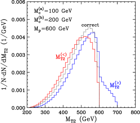
This is illustrated in Fig. 4, where we show results for the event topology of Fig. 3(b) with a mass spectrum as follows: GeV, GeV and GeV. The test children masses are taken to be the true masses: and . The dotted black distribution is the unit-normalized true distribution, where one ignores the combinatorial problem and uses the Monte Carlo information to make the correct association. The red histogram shows the unit-normalized distribution of the variable defined in (56). We see that the definition (56) preserves the corresponding endpoint:
| (57) |
Of course, we can also consider the alternative combination
| (58) |
whose unit-normalized distribution is shown in Fig. 4 with the blue histogram. One can see that some of the wrong combination entries in the histogram violate the original endpoint , yet there is still a well defined endpoint
| (59) |
Strictly speaking, in our analysis in the next sections, we only need to study the endpoint (57), which contains the relevant information about the physical endpoint. At the same time, with our convention (53) for the children masses, we only need to concentrate on the upper half of the plane. However, for completeness we shall also present results for the endpoint (59), and we shall use the lower () half of the plane to show those. Thus the endpoint shown in our plots below should be interpreted as follows
| (60) |
4 The simplest event topology: one SM particle on each side
In this section, we consider the simplest topology with a single visible particle on each side of the event. We already introduced this example in Section 3.4, along with its event topology in Fig. 3(a). In Section 4.1 below we first discuss an asymmetric case with different children. Later in Section 4.2 we consider a symmetric situation with identical children masses. The mass spectra for these two study points are listed in Table 1.
Spectrum Case I Different children 250 500 600 II Identical children 100 100 300
4.1 Asymmetric case
Before we present our numerical results, it will be useful to derive an analytical expression for the asymmetric endpoint (42) in terms of the corresponding physical spectrum of Table 1 and the two test children masses and . Our result will generalize the corresponding formula derived in [68] for the symmetric case of and no upstream momentum (). For the event topology of Fig. 3(a) the endpoint is always obtained from the balanced solution and is given by [68]
| (61) |
Here we made use of the convenient shorthand notation introduced in [85] for the relevant combination of physical masses
| (62) |
The parameter defined in (62) is simply the transverse momentum of the (massless) visible particle in those events which give the maximum value of [97]. Squaring (61), we can equivalently rewrite it as
| (63) |
Now let us derive the analogous expressions for the asymmetric case . Just like the symmetric case, the asymmetric endpoint also comes from a balanced solution and is given by
| (64) |
where the parameters and were already defined in (35) and (36), while is now the geometric average of the corresponding individual parameters
| (65) |
It is easy to check that in the symmetric limit
| (66) |
eq. (64) reduces to its symmetric counterpart (63), as it should.
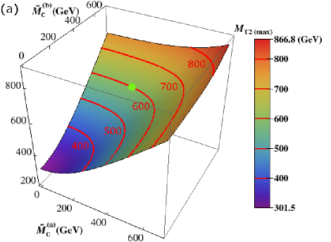
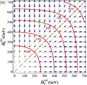
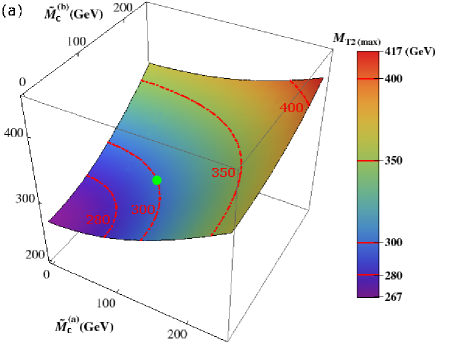
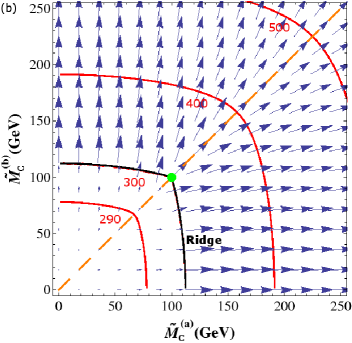
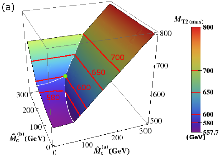
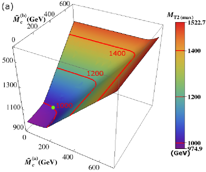
We are now ready to present our numerical results for the event topology of Fig. 3(a). We first take the asymmetric mass spectrum I from Table 1 and consider the case with no upstream momentum, when formula (64) applies. Fig. 5 shows the corresponding endpoint as a function of the two test children masses and . In panel (a) we present a three dimensional view, while in panel (b) we show a contour plot projection on the plane (red contour lines). On either panel, the green dot marks the true values of the children masses, and . Panel (b) also shows a gradient plot, where longer (shorter) arrows imply steeper (gentler) slope. The symmetric endpoint of eq. (61) can be obtained by going along the diagonal orange line in Fig. 5(b). We remind the reader that the endpoint plotted in Fig. 5 should be interpreted as in eq. (60).
Fig. 5 illustrates the first basic property of the asymmetric variable, which was discussed in Sec. 3.3.1. The endpoint allows us to find one relation between the two children masses and and the parent mass , and in order to do so, we do not have to assume equality of the children masses, as is always done in the literature. The crucial advantage of our approach, in which we allow the two children masses to be arbitrary, is its generality and model-independence. It allows us to extract the basic information contained in the endpoint, without muddling it up with additional theoretical (and unproven) assumptions.
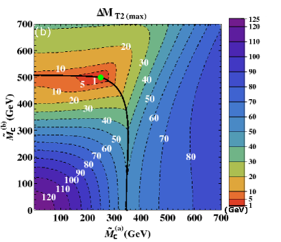
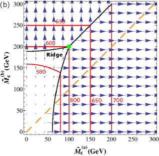
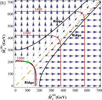
Unfortunately, to go any further and determine each individual mass, we must make use of the additional properties discussed in Secs. 3.3.2 and 3.3.3. In the case of the simplest event topology of Fig. 3(a) considered here, they both require the presence of some upstream momentum [67, 85]. As a proof of concept, we now reconsider the same type of events, but with a fixed upstream momentum of TeV. (The upstream momentum may be due to initial state radiation, or decays of heavier particles upstream.) The corresponding results are shown in Fig. 6.
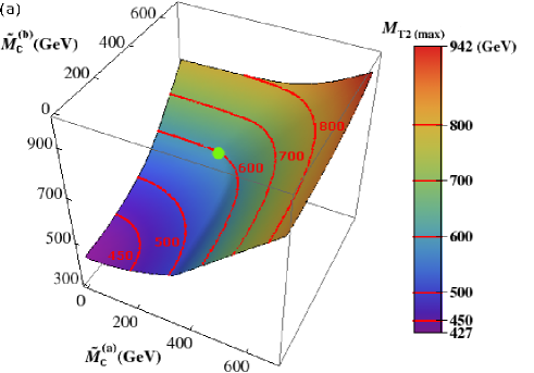
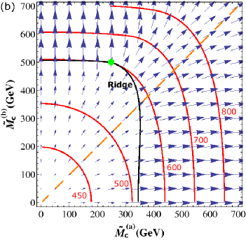
Fig. 6 demonstrates the second basic property of the asymmetric variable discussed in Sec. 3.3.2. Unlike the result shown in Fig. 5(a), which was perfectly smooth, this time the function in Fig. 6(a) shows a ridge, corresponding to the slope discontinuity marked with the black solid line in Fig. 6(b). The most important feature of the ridge is the fact that it passes through the green dot marking the true values of the children masses. Notice that applying the traditional symmetric approach in this case will give a completely wrong result. If we were to assume equal children masses from the very beginning, we will be constrained to the diagonal orange line in Fig. 6(b). The endpoint will then still exhibit a kink, but the kink will be in the wrong location. In the example shown in Fig. 6(b), we will underestimate the parent mass, while for the child mass we will find a value which is somewhere in between the two true masses and .
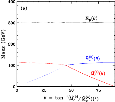
Using the ridge information, we now know an additional relation among the children masses, which allows us to express all three masses in terms of a single unknown parameter , as illustrated in Fig. 7(a).
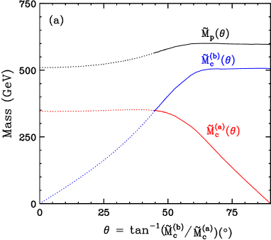
Let us choose to parametrize the ridge by the polar angle in the plane:
| (67) |
Using the ridge information from Fig. 6, we can then find all three masses as a function of . The result is shown in Fig. 7(a). The mass of the lighter child is plotted in red, the mass of the heavier child is plotted in blue, while the parent mass is plotted in black. With our convention (53) for the children masses, only values of are physical, and the corresponding masses are shown with solid lines. The dotted lines in Fig. 7(a) show the extrapolation into the unphysical region .
Fig. 7(a) has some important and far reaching implications. For example, one may now start asking the question: Are there really any massive invisible particles in those events, or is the missing energy simply due to neutrino production [21]? The ridge results shown in Fig. 7(a) begin to provide the answer to that quite fundamental question. According to Fig. 7(a), for any value of the (still unknown) parameter , the two children particles cannot be simultaneously massless. This means that the missing energy cannot be simply due to neutrinos, i.e. there is at least one new, massive invisible particle produced in the missing energy events. At this point, we cannot be certain that this is a dark matter particle, but establishing the production of a WIMP candidate at a collider is by itself a tremendously important result. Notice that while we cannot be sure about the masses of the children, the parent mass is determined with a very good precision from Fig. 7(a): the function is almost flat and rather insensitive to the particular value of 141414 Interestingly, for the example in Fig. 7(a), the maximum value of happens to give the true parent mass , but we have checked that this is a coincidence and does not hold in general for other examples which we have studied..
Once we have proved that some kind of WIMP production is going on, the next immediate question is: how many such WIMP particles are present in the data – one or two? Unfortunately, the ridge analysis of Fig. 7(a) alone cannot provide the answer to this question, since the value of is still undetermined. If , one of the missing particles is massless, which is consistent with a SM neutrino. Therefore, if were indeed , the most plausible explanation of this scenario would be that only one of the missing particles is a genuine WIMP, while the other is a SM neutrino. On the other hand, almost any other value of would guarantee that there are two WIMP candidates in each event. In that case, the next immediate question is: are they the same or are they different? Fortunately, our asymmetric approach will allow answering this question in a model-independent way. If is determined to be , the two WIMP particles are the same, i.e. we are producing a single species of dark matter. On the other hand, if , then we can be certain that there are not one, but two different WIMP particles being produced.
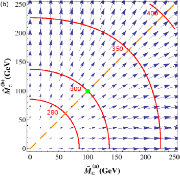
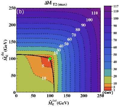
We see that in order to completely understand the physics behind the missing energy signal, we must determine the value of , i.e. we must find the exact location of the true children masses along the ridge. One of our main results in this paper is that this can be done by using the third property discussed in Sec. 3.3.3. The idea is illustrated in Fig. 7(b), where we show a contour plot in the plane of the quantity defined in eq. (48), for a fixed TeV. This plot is obtained simply by taking the difference between Fig. 6(a) and Fig. 5(a). (A more practical method for obtaining this information was proposed in [100].) Recall that the function was introduced in order to quantify the invariance of the endpoint, and it is expected that vanishes at the correct values of the children masses (see eq. (50)). This expectation is confirmed in Fig. 7(b), where we find the minimum (zero) of the function exactly at the right spot (marked with the green dot) along the ridge. Thus the function in Fig. 7(b) completely pins down the spectrum, and in this case would reveal the presence of two different WIMP particles, with unequal masses . Our analysis thus shows that colliders can not only produce a WIMP dark matter candidate and measure its mass, as discussed in the existing literature, but they can do a much more elaborate dark matter particle spectroscopy, as advertized in the title. In particular, they can probe the number and type of missing particles, including particles from subdominant dark matter species, which are otherwise unlikely to be discovered experimentally in the usual dark matter searches.
4.2 Symmetric case
While in our approach the two children masses and are treated as independent inputs, this, of course, does not mean that the approach is only valid in cases when the children masses are different to begin with. The techniques discussed in the previous subsection remain applicable also in the more conventional case when the children are identical, i.e. when colliders produce a single dark matter component. In order to illustrate how our method works in that case, we shall now work out an example with equal children masses. We still consider the simplest event topology of Fig. 3(a), but with the symmetric mass spectrum II from Table 1. We then repeat the analysis done in Figs. 5, 6, and 7 and show the corresponding results in Figs. 8, 9 and 10.
The conclusions from this exercise are very similar to what we found earlier in Sec. 4.1 for the asymmetric case. The endpoint still provides one relation among the two children masses and and the parent mass . This relation is shown in Fig. 8 (Fig. 9) for the case without (with) upstream momentum . As seen in Fig. 8, in the absence of any upstream , the function is smooth and reveals nothing about the children masses. However, the presence of upstream momentum significantly changes the picture and the function again develops a ridge, which is clearly visible151515We caution the reader that here we are presenting only a proof of concept. In the actual analysis the ridge may be rather difficult to see, for a variety of reasons - detector resolution, finite statistics, combinatorial and SM backgrounds, etc. Nevertheless, we expect that the ridge will be just as easily observable as the traditional kink in the symmetric endpoint. If the kink can be seen in the data, the ridge can be seen too, and there is no reason to make the assumption of equal children masses. Conversely, if the kink is too difficult to see, the ridge will remain hidden as well. in both the three-dimensional view of Fig. 9(a), as well as the gradient plot in Fig. 9(b). The ridge information now further constrains the children masses to the black solid line in Fig. 9(b), leaving only one unknown degree of freedom. Parametrizing it with the polar angle as in (67), we obtain the spectrum as a function of , as shown in Fig. 10(a).
Once again we find the fortuitous result that in spite of the remaining arbitrariness in the value of , the parent mass is very well determined, since is a very weakly varying function of . Furthermore, both Fig. 9(a) and Fig. 9(b) exhibit a high degree of symmetry under , which is a good hint that the children are in fact identical. This suspicion is confirmed in Fig. 10(b), where we find that the dependence disappears at the symmetric point GeV, revealing the true masses of the two children.
In the two examples considered so far in Sections 4.1 and 4.2, we used a fixed finite value of the upstream transverse momentum TeV, which is probably rather extreme — in realistic models, one might expect typical values of on the order of several hundred GeV. However, things begin to get much more interesting if one were to consider even larger values of . On the one hand, the ridge feature becomes sharper and easier to observe [85]. More importantly, the ridge structure itself is modified, and a second set of ridgelines appears161616A keen observer may have already noticed a hint of those in Figs. 7(b) and 10(b). at sufficiently large . All ridgelines intersect precisely at the point marking the true values of the children masses, thus allowing the complete determination of the mass spectrum by the ridge method alone. This procedure was demonstrated explicitly in Ref. [96], which investigated the extreme case of for a study point with different parents and identical children. The assumption of justified the use of a “decoupling argument”, in which the two branches and are treated independently, allowing the derivation of simple analytical expressions for the endpoint [96]. In Appendix A we reproduce the analogous analytical results at for the case of interest here (identical parents and different children) and study in detail the dependence of the ridgelines. Unfortunately, we find that the values of necessary to reveal the additional ridge structure, are too large to be of any interest experimentally. On the positive side, the invariance method discussed in Sec. 2.3.3 does not require such extremely large values of and can in principle be tested in more realistic experimental conditions.
4.3 Mixed case
For simplicity, so far in our discussion we have been studying only one type of missing energy events at a time. In reality, the missing energy sample may contain several different types of events, and the corresponding measurements will first need to be disentangled from each other.
For concreteness, consider the inclusive pair production of some parent particle , which can decay either to a child particle of mass , or a different child particle of mass . Let the corresponding branching fractions be and , i.e. and . Furthermore, let decay invisibly171717If decays visibly, then the respective types of events can in principle be sorted by their signature. to . Such a situation can be easily realized in supersymmetry, for example, with the parent being a squark, a slepton, or a gluino, the heavier child being a Wino-like neutralino and the lighter child being a Bino-like neutralino . The heavier neutralino has a large invisible decay mode , if its mass happens to fall between the sneutrino mass and the left-handed slepton mass: .
Let us start with a certain total number of events in which two parent particles have been produced. Then the missing energy sample will contain symmetric events where the two children are and , symmetric events where the two children are and , and asymmetric events where the two children are and . How can one analyze such a mixed event sample with a single variable?
The black histogram in Fig. 11 shows the unit-normalized distribution for the whole (mixed) event sample (for convenience, we do not show the zero bin [100]).
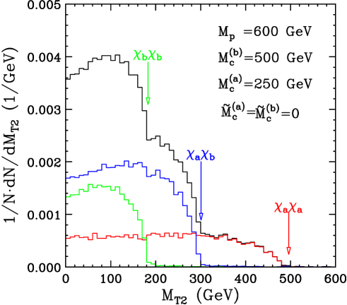
For this plot, we used the asymmetric mass spectrum I from table 1: GeV, GeV and GeV, and chose zero test masses for the children . For definiteness, we fixed equal branching fractions , so that the relative normalization of the three individual samples is . Fig. 11 shows that the observable distribution is simply a superposition of the distributions of the three individual samples , and , which are shown with the red, blue and green histograms, correspondingly. Each individual sample exhibits its own endpoint, marked with a vertical arrow, which can also be seen in the combined distribution. Using eq. (64), the three endpoints are found to be
| (68) | |||||
| (69) | |||||
| (70) |
Now suppose that all three endpoints (68-70) are seen in the data. Their interpretation is far from obvious, and in fact, there will be different competing explanations. If one insists on the single missing particle hypothesis, there can be only one type of child particle, and the only way to get three different endpoints in Fig. 11 is to have production of three different pairs of parent particles, each of which decays in exactly the same way. Since the three parent masses are a priori unrelated, one does not expect any particular correlation among the three observed endpoints (68-70). Now consider an alternative explanation where we produce a single type of parents, but have two different children types. This situation also gives rise to three different event topologies, with three different endpoints, as we just discussed. However, now there is a predicted relation among the three endpoints, which follows simply from eqs. (68-70):
| (71) |
If the parents are the same and the children are different, this relation must be satisfied. If the parents are different and the children are the same, a priori there is no reason why eq. (71) should hold, and if it does, it must be by pure coincidence. The prediction (71) therefore is a direct test of the number of children particles. Another test can be performed if we could estimate the individual event counts , and , although this appears rather difficult, due to the unknown shape of the distributions in Fig. 11. In the asymmetric example discussed here, we have another prediction, namely
| (72) |
which is another test of the different children hypothesis. Notice that eq. (72) holds regardless of the branching fractions and , although if one of them dominates, the two endpoints which require the other (rare) decay may be too difficult to observe.
Of course, the ultimate test of the single missing particle hypothesis is the behavior of the intermediate endpoint in Fig. 11 corresponding to the asymmetric events of type . Applying either one of the two mass determination methods discussed earlier in Figs. 7 and 10, we should find that is a result of asymmetric events, indicating the simultaneous presence of two different invisible particles in the data.
5 A more complex event topology: two SM particles on each side
In this section, we consider two more examples: the off-shell event topology of Fig. 3(b) is discussed in Sec. 5.1, while the on-shell event topology of Fig. 3(c) is discussed in Sec. 5.2. (For simplicity, we do not consider any in this section.) Now there are two visible particles in each leg, which form a composite visible particle of varying mass . In general, by studying the invariant mass distribution of , one should be able to observe two different invariant mass endpoints, suggesting some type of an asymmetric scenario.
5.1 Off-shell intermediate particle
Here we concentrate on the example of Fig. 3(b). Since the intermediate particle is offshell, the maximum kinematically allowed value for is given by eq. (51).
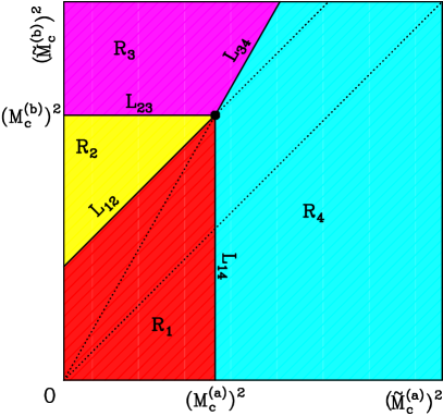
Recall that for the simple topology of Fig. 3(a) discussed in the previous section, the endpoint (64) always corresponded to a balanced solution. More precisely, the variable was maximized for a momentum configuration in which was given by the balanced solution (34). However, in this section we shall find that for the more complex topologies of Figs. 3(b) and 3(c), the endpoint may result from one of four different cases altogether: two different balanced solutions, which we shall label as and , or the unbalanced solutions and discussed in Sec. 3.2. Depending on the type of solution giving the endpoint , the parameter plane divides into the three regions181818The fourth case of the balanced solution happens to coincide with the two unbalanced solutions along the boundary between and . shown in Fig. 12.
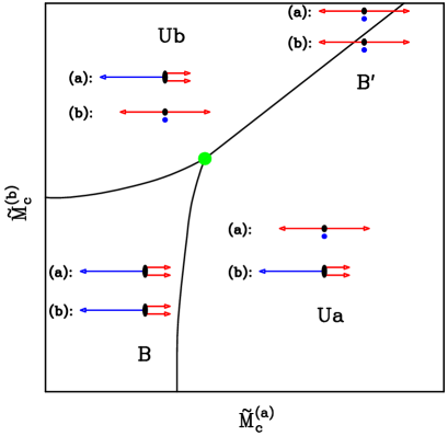
The green dot in Fig. 12 denotes the true children masses in this parameter space. Within each region, we show the relevant momentum configuration for the visible particles (red arrows) and the children particles (blue arrows) in each leg ( or ). The momenta are quoted in the “back-to-back boosted” (BB) frame [68], in which the two parents are at rest. The length of an arrow is indicative of the magnitude of the momentum. A blue dot implies that the corresponding daughter is at rest and therefore the two visible particles are emitted back-to-back. The two balanced solutions are denoted as and , while the two unbalanced solutions are and . The black solid lines represent phase changes between different solution types and delineate the expected locations of the ridges in the function shown in Fig. 13 below. Perhaps the most striking feature of Fig. 12 is that the three (in fact, all four) regions come together precisely at the green dot marking the true values of the two children masses. The boundaries of the regions shown in Fig. 12 will manifest themselves as the locations of the ridges (i.e. gradient discontinuities) in the function. Therefore, we expect that by studying the ridge structure and finding its “triple” point, one will be able to completely determine the mass spectrum.
We shall now give analytical formulas for the endpoint in each of the four regions of Fig. 12. We begin with the two balanced solutions and , for which the event-by-event balanced solution for is given by eq. (34). In the parameter space region of Fig. 12 which is adjacent to the origin, we find the balanced configuration , in which all visible particles have the same direction in the BB frame. As a result, we have
| (73) |
and
| (74) |
Substituting eqs. (73) and (74) in the balanced solution (34), where we should take the plus sign, we obtain
| (75) |
which we recognize as the balanced solution (64) found for the decay topology of Fig. 3(a).
Moving away from the origin in Fig. 12, we find a second balanced solution along the boundary of the unbalanced regions and . In this case the visible particles are back-to-back, and their invariant mass is maximized:
| (76) |
and correspondingly
| (77) |
Substituting eqs. (76) and (77) in the balanced solution (34), we obtain the -type endpoint as
| (78) |
The corresponding formulas for the unbalanced cases and are obtained by taking the maximum value for the invariant mass of the visible particles in the corresponding decay chain:
| (79) | |||||
| (80) |
The corresponding formula for is then given by
| (81) | |||||
| (82) |
One can now use the analytical results (75), (78), (81) and (82) to understand the ridge structure shown in Fig. 12. For example, the boundary between the and regions is parametrically given by the condition
| (83) |
while the boundary between the and regions is parametrically given by
| (84) |
On the other hand, the boundary
| (85) |
between the two unbalanced regions and is quite interesting. The parametric equation (85) is nothing but a straight line in the plane:
| (86) |
as seen in Fig. 12.
It is now easy to understand the triple point structure in Fig. 12. The triple point is obtained by the merging of all three boundaries (83), (84) and (85), i.e. when
| (87) |
It is easy to check that and identically satisfy these equations, thereby proving that the triple intersection of the boundaries seen in Fig. 12 indeed takes place at the true values of the children masses.
These results are confirmed in our numerical simulations.
In Fig. 13 we present (a) a three dimensional view and (b) a gradient plot of the ridge structure found in events with the off-shell topology of Fig. 3(b). The mass spectrum for this study point was fixed as in Fig. 4, namely GeV, GeV and GeV. Since the ridge structure for this topology does not require the presence of upstream momentum, for simplicity we consider only events with . The ridge pattern is clearly evident in Fig. 13(a), which shows a three-dimensional view of the endpoint function . It is even more apparent in Fig. 13(b), where one can see a sharp gradient change along the ridge lines: in regions and , the corresponding gradient vectors point in trivial directions (either horizontally or vertically), in accord with eqs. (81)-(82). On the other hand, the gradient in region is very small, and the endpoint function is rather flat. The green dot marks the location of the true children masses ( GeV, GeV) and is indeed the intersection point of the three ridgelines. As expected, the corresponding at that point is the true parent particle mass GeV.
At this point, it is interesting to ask the question, what would be the outcome of this exercise if one were to make the usual assumption of identical children, and apply the traditional symmetric to this situation. The answer can be deduced from Fig. 13(b), where the diagonal orange dotdashed line corresponds to the usual assumption of . In that case, one still finds a kink, but at the wrong location: in Fig. 13(b) the intersection of the diagonal orange line and the solid black ridgeline occurs at GeV and the corresponding parent mass is GeV. Therefore, the traditional kink method can easily lead to a wrong mass measurement. Then the only way to know that there was something wrong with the measurement would be to study the effect of the upstream momentum and see that the observed kink is not invariant under .
We should note that, depending on the actual mass spectrum, the two-dimensional ridge pattern seen in Figs. 12 and 13(b) may look very differently. For example, the balanced region may or may not include the origin. One can show that if
| (88) |
the boundary between and does not cross the axis. In this case the diagonal line in Fig. 13(b) does not cross any ridgelines and the traditional approach will not produce any kink structure, in contradiction with one’s expectations. This exercise teaches us that the failsafe approach to measuring the masses in missing energy events is to apply from the very beginning the asymmetric concept advertized in this paper.
5.2 On-shell intermediate particle
Our final example is the on-shell event topology illustrated in Fig. 3(c). Now there is an additional parameter which enters the game — the mass of the intermediate particle in the -th decay chain. As a result, the allowed range of invariant masses for the visible particle pair on each side is limited from above by eq. (52).
In this case we find that the endpoint exhibits a similar phase structure as the one shown in Fig. 12.
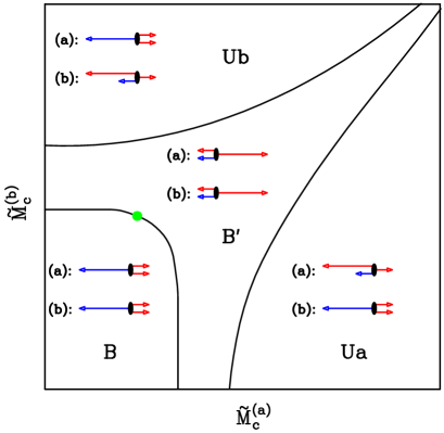
One particular pattern is illustrated in Fig. 14, which exhibits the same four regions , , and seen in Fig. 12. The difference now is that region is considerably expanded, and as a result, region does not have a common border with regions and any more. The triple point of Fig. 12 has now disappeared and the correct values of the children masses now lie somewhere on the border between regions and , but their exact location along this ridgeline is at this point unknown.
Just like we did for the off-shell case in Sec. 5.1, we shall now present analytical formulas for the endpoint in each region of Fig. 14. In the balanced region , we find the same results (73-75) as in the off-shell case considered in the previous Section 5.1. The other balanced region is characterized by
| (89) |
where is given by eq. (52), and
| (90) | |||||
The formula for the endpoint in region is then simply obtained by substituting (89) and (90) into the balanced solution (34).
Finally, the endpoint in the unbalanced regions and is given by
| (91) | |||||
| (92) |
where and are given by eq. (52).
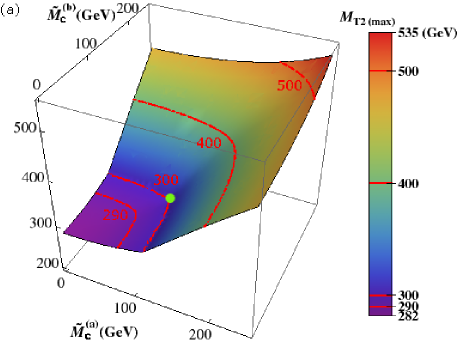
In Fig. 15 we present our numerical results in this on-shell scenario. The mass spectrum is fixed as: GeV, GeV, GeV and TeV, and we still do not include the effects of any upstream momentum. Fig. 15(a) shows the three-dimensional view of the endpoint function , which exhibits three different sets of ridges, which are more easily seen in the gradient plot of Fig. 15(b). As usual, the green dot marks the true children masses. Fig. 15(b) shows that the ridgeline separating the two balanced regions and does go through the green dot and thus reveals a relationship between the two children masses, leaving the ridgeline parameter as the only remaining unknown degree of freedom. However, unlike the off-shell case of Sec. 5.1, now there is no special point on this ridgeline, and we cannot completely pin down the masses by the ridge method. Thus, in order to determine all masses in the problem, one must use an additional piece of information, for example the visible invariant mass endpoint (52) or the invariance method suggested in Sec. 3.3.3.
6 Summary and conclusions
Cosmological observations hint towards the existence of one or more hypothetical dark matter particles. The start of the Large Hadron Collider may offer an unique opportunity to produce and study dark matter in a high-energy experimental laboratory. Unfortunately, the dark matter signatures at colliders always involve missing transverse energy. Such events will be quite challenging to fully reconstruct and/or interpret. All previous studies have made (either explicitly or implicitly) the assumption that each event has two identical missing particles. Our main point in this paper is that this assumption is unnecessary, and by suitable modifications of the existing analysis techniques one can in principle test both the number and the type of missing particles in the data. Our proposal here was to modify the Cambridge variable [50] by treating each children mass as an independent input parameter. In this approach, one obtains the endpoint as a function of the two children masses and , and proceeds to study its properties. The two most important features of the thus obtained function , identified in this paper, were the following:
-
•
The function exhibits a ridge structure (i.e. a gradient discontinuity), as illustrated with specific examples in Figs. 6, 9, 13 and 15. The point corresponding to the correct children masses always lies on a ridgeline, thus the ridgelines provide a model-independent constraint among the children masses, just like the endpoint provides a model-independent constraint on the masses of the child(ren) and the parent.
-
•
In general, the endpoint function also depends on the value of the upstream transverse momentum in the event: . However, the dependence disappears completely for precisely the right values of the children masses, as seen in the examples of Figs. 7(b) and 10(b). This provides a second, quite general and model-independent, method for measuring the individual particle masses in such missing energy events.
Before we conclude, we shall discuss a few other possible applications of the asymmetric idea, besides the examples already considered in the paper.
-
1.
Invisible decays of the next-to-lightest particle. Most new physics models introduce some new massive and neutral particle which plays the role of a dark matter candidate. Often the very same models also contain other, heavier particles, which for collider purposes behave just like a dark matter candidate: they decay invisibly and result in missing energy in the detector. For example, in supersymmetry one may find an invisibly decaying sneutrino , in UED one finds an invisibly decaying KK neutrino , etc. These scenarios can easily generate an asymmetric event topology. For example, consider the strong production of a squark () pair, as illustrated in Fig. 16(a). One of the squarks subsequently decays to the second lightest neutralino , which in turn decays to the lightest neutralino by emitting two SM fermions (or ). The other squark decays to a chargino , which then decays to a sneutrino as . Since can only decay invisibly, we obtain the asymmetric event topology outlined with the blue box in Fig. 16(a). The two squarks are the parents, the lightest neutralino is the first child, and the sneutrino is the second child.
Figure 16: Event topology for the two examples discussed in Section 6. The black solid lines represent SM particles which are visible in the detector while red solid lines represent particles at intermediate sages. The missing particles are denoted by dotted lines. (a) Squark pair production with decay chains terminating in two different invisible particles ( and , correspondingly). In this case decays invisibly. (b) The subsystem variable applied to events. The -boson in the lower leg is treated as a child particle and can decay either hadronically or leptonically. -
2.
Applying to an asymmetric subsystem. One can also apply the idea even to events in which there is only one (or even no) missing particles to begin with. Such an example is shown in Fig. 16(b), where we consider production in the dilepton or semi-leptonic channel. In the first leg we can take as our visible system and the neutrino as the invisible particle, while in the other leg we can treat the -jet as the visible system and the -boson as the child particle. In this case, there still should be a ridge structure revealing the true , and masses.
- 3.
In conclusion, our work shows that the concept can be easily generalized to decay chains terminating in two different daughter particles. Nevertheless, the methods discussed in this paper allow to extract all masses involved in the decays, at least as a matter of principle. We believe that such methods will prove extremely useful, if a missing energy signal of new physics is seen at the Tevatron or the LHC.
Acknowledgments.
We are grateful to A. J. Barr, B. Gripaios, C. G. Lester, and L. Pape for their insightful and stimulating comments. All authors would like to thank the Fermilab Theoretical Physics Department for warm hospitality and support at various stages during the completion of this work. This work is supported in part by a US Department of Energy grant DE-FG02-97ER41029. KK is supported in part by the DOE under contract DE-AC02-76SF00515.Appendix A Appendix: The asymmetric in the limit of infinite
In this appendix we revisit our previous two examples from Sections 4.1 and 4.2, this time considering the infinitely large limit [96]. While this situation is impossible to achieve in a real experiment, its advantage is that it can be treated by analytical means. In the limit, the “decoupling argument” of Ref. [96] holds, and one finds the following analytical expression for the endpoint as a function of the two test children masses and :
| (A.1) |
where the four defining regions , are shown in Fig. 17 and are defined as follows:
| (A.2) | |||||
| (A.3) | |||||
| (A.4) | |||||
| (A.5) |
Since the functional expression for within each region is different, there is in general a gradient discontinuity when crossing from one region into the next. Therefore, the ridges on the hypersurface will appear along the common boundaries of the four regions . Let us denote by the boundary between regions and . As indicated in Fig. 17, each is a straight line in the parameter space of the children test masses squared and is given by
| (A.6) | |||||
| (A.7) | |||||
| (A.8) | |||||
| (A.9) |
As seen in Fig. 17, all four lines meet at the true children mass point , , where in turn the endpoint gives the true parent mass , in accordance with eq. (43).
With those preliminaries, we are now in a position to revisit our two examples from Sections 4.1 and 4.2. Figs. 18 and 19 are the corresponding analogues of Figs. 6 and 9 in the case of infinite . Comparing with our earlier results, we notice both quantitative and qualitative changes in the ridge structure. First, the smooth ridge in Fig. 6(b) (Fig. 9(b)) has now been deformed into two straight line segments, one horizontal () and the other vertical (), which meet at an angle of precisely at the true values of the children masses. More importantly, Figs. 18 and 19 now exhibit another pair of ridges and (plotted in red in Figs. 18(b) and 19(b)), which were absent from the earlier figures in Section 4. The system of four ridges seen in Figs. 18(a) and 19(a) is very similar to the crease structure observed in Ref. [96]. We thus confirm the result of Ref. [96] that in the infinite limit there exist four different ridges, whose common intersection point reveals the true masses of the parent and children particles.
At this point it is instructive to contrast the two sets of ridgelines: and (shown in Figs. 18(b) and 19(b) in black) versus and (shown in Figs. 18(b) and 19(b) in red). The boundaries and separate the union of regions and from the union of regions and . Along those boundaries, we observe a transition in the configuration of visible momenta which yields the maximum possible value of . More precisely, in regions and we find that the visible momenta for are parallel to the direction of the upstream momentum , while in regions and we find that are anti-parallel to . This fact remains true even at finite values of , which is why the ridgelines and could also be seen in the earlier plots from Sec. 4 at finite TeV.
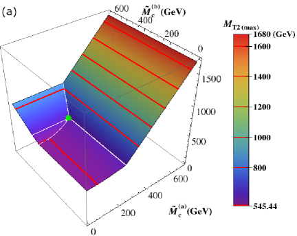
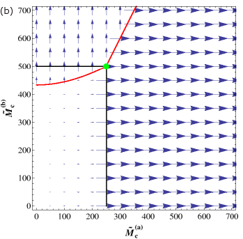
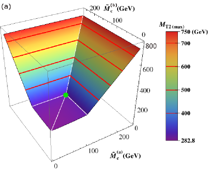
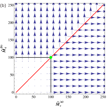
On the other hand, the ridgelines and shown in red in Figs. 18(b) and 19(b) are due to the “decoupling argument” [96], which is strictly valid only in the infinite limit. This is why these ridges become apparent only at very large values of , and are gradually smeared out at smaller .
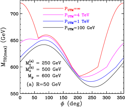
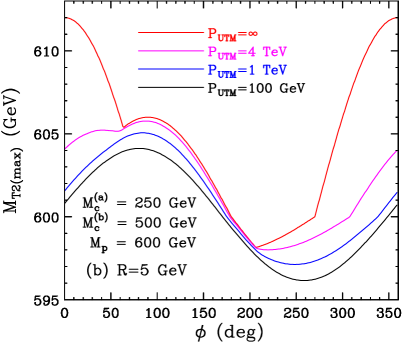
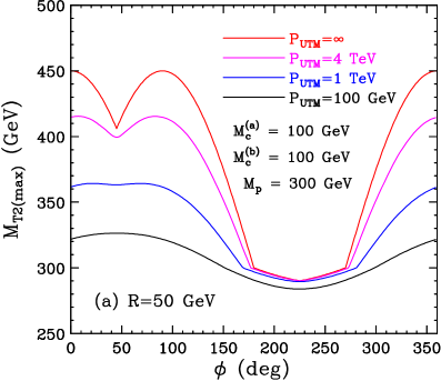
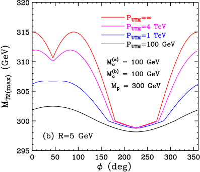
The evolution of the ridge structure as a function of is shown in Figs. 20 and 21. In order to compare the sharpness of the four ridges, we choose to vary the test children masses and along a circle centered on their true values and with a fixed radius . Such a circle is guaranteed to cross all four ridges, and can be parameterized in terms of an angular coordinate as follows
| (A.10) | |||||
| (A.11) |
Then in Fig. 20 (Fig. 21) we plot the asymmetric endpoint , as a function of the angular variable , for the case of mass spectrum I studied in Section 4.1 (mass spectrum II studied in Section 4.2). The radius is taken to be GeV in panels (a) and GeV in panels (b). We present results for four different choices of the upstream momentum: GeV (black lines), TeV (blue lines), TeV (magenta lines), and (red lines). Notice that the red lines at in Figs. 20 and 21 are directly correlated to the three-dimensional plots of Figs. 18 and 19, while the blue lines at TeV in Figs. 20 and 21 are directly correlated to the three-dimensional plots of Figs. 6 and 9.
Each one of the previously discussed ridges manifests itself as a kink in Figs. 20 and 21. Indeed, the red lines for reveal four clear kinks, which (from left to right) correspond to the ridgelines , , , and . Using eqs. (A.6-A.9), it is easy to find the expected location of each kink in the limit: for Fig. 20(a), for Fig. 20(b), and for Figs. 21(a) and 21(b). However, as the upstream momentum is lowered to more realistic values, the kinks gradually wash out, albeit to a different degree. As anticipated from our earlier results, the smearing effect is quite severe for and , and by the time we reach TeV, those two kinks have completely disappeared. On the other hand, and are affected to a lesser degree by the smearing effect and are still visible at TeV, but by GeV they are essentially gone as well. Notice that the variation in affects not only the sharpness of the kinks, but also their location. This was to be expected, since we already saw that the shape of the ridge is different at TeV and : compare the black ridge lines in Figs. 6(b) and 9(b) to those in Figs. 18(b) and 19(b). Finally, as a curious fact we notice that the results shown in panels (a) and panels (b) of Figs. 20 and 21 are approximately related by a simple scaling with a constant factor.
References
- [1] G. Jungman, M. Kamionkowski and K. Griest, “Supersymmetric dark matter,” Phys. Rept. 267, 195 (1996) [arXiv:hep-ph/9506380].
- [2] G. Servant and T. M. P. Tait, “Is the lightest Kaluza-Klein particle a viable dark matter candidate?,” Nucl. Phys. B 650, 391 (2003) [arXiv:hep-ph/0206071].
- [3] F. Burnell and G. D. Kribs, “The abundance of Kaluza-Klein dark matter with coannihilation,” Phys. Rev. D 73, 015001 (2006) [arXiv:hep-ph/0509118].
- [4] K. Kong and K. T. Matchev, “Precise calculation of the relic density of Kaluza-Klein dark matter in universal extra dimensions,” JHEP 0601, 038 (2006) [arXiv:hep-ph/0509119].
- [5] H. C. Cheng and I. Low, “TeV symmetry and the little hierarchy problem,” JHEP 0309, 051 (2003) [arXiv:hep-ph/0308199].
- [6] A. Birkedal, A. Noble, M. Perelstein and A. Spray, “Little Higgs dark matter,” Phys. Rev. D 74, 035002 (2006) [arXiv:hep-ph/0603077].
- [7] A. Birkedal, K. Matchev and M. Perelstein, “Dark matter at colliders: A model-independent approach,” Phys. Rev. D 70, 077701 (2004) [arXiv:hep-ph/0403004].
- [8] J. L. Feng, S. Su and F. Takayama, “Lower limit on dark matter production at the Large Hadron Collider,” Phys. Rev. Lett. 96, 151802 (2006) [arXiv:hep-ph/0503117].
- [9] E. A. Baltz, M. Battaglia, M. E. Peskin and T. Wizansky, “Determination of dark matter properties at high-energy colliders,” Phys. Rev. D 74, 103521 (2006) [arXiv:hep-ph/0602187].
- [10] D. J. H. Chung, L. L. Everett, K. Kong and K. T. Matchev, “Connecting LHC, ILC, and Quintessence,” JHEP 0710, 016 (2007) [arXiv:0706.2375 [hep-ph]].
- [11] C. F. Berger, J. S. Gainer, J. L. Hewett, T. G. Rizzo and B. Lillie, “The LHC Inverse Problem, Supersymmetry, and the ILC,” Phys. Lett. B 677, 48 (2009) [arXiv:0711.1374 [hep-ph]].
- [12] H. Baer and X. Tata, “Dark matter and the LHC,” arXiv:0805.1905 [hep-ph].
- [13] S. Arrenberg, L. Baudis, K. Kong, K. T. Matchev and J. Yoo, “Kaluza-Klein Dark Matter: Direct Detection vis-a-vis LHC,” Phys. Rev. D 78, 056002 (2008) [arXiv:0805.4210 [hep-ph]].
- [14] C. F. Berger, J. S. Gainer, J. L. Hewett and T. G. Rizzo, “Supersymmetry Without Prejudice,” JHEP 0902, 023 (2009) [arXiv:0812.0980 [hep-ph]].
- [15] H. Baer, E. K. Park and X. Tata, “Collider, direct and indirect detection of supersymmetric dark matter,” New J. Phys. 11, 105024 (2009) [arXiv:0903.0555 [hep-ph]].
- [16] L. Roszkowski, R. Ruiz de Austri and R. Trotta, “Efficient reconstruction of CMSSM parameters from LHC data - A case study,” arXiv:0907.0594 [hep-ph].
- [17] A. Birkedal et al., “Testing cosmology at the ILC,” In the Proceedings of 2005 International Linear Collider Workshop (LCWS 2005), Stanford, California, 18-22 Mar 2005, pp 0708 [arXiv:hep-ph/0507214].
- [18] G. Belanger, O. Kittel, S. Kraml, H. U. Martyn and A. Pukhov, “Neutralino relic density from ILC measurements in the CPV MSSM,” Phys. Rev. D 78, 015011 (2008) [arXiv:0803.2584 [hep-ph]].
- [19] N. Bernal, A. Goudelis, Y. Mambrini and C. Munoz, “Determining the WIMP mass using the complementarity between direct and indirect searches and the ILC,” JCAP 0901, 046 (2009) [arXiv:0804.1976 [hep-ph]].
- [20] P. Konar, K. Kong, K. T. Matchev and M. Perelstein, “Shedding Light on the Dark Sector with Direct WIMP Production,” New J. Phys. 11, 105004 (2009) [arXiv:0902.2000 [hep-ph]].
- [21] S. Chang and A. de Gouvea, “Neutrino Alternatives For Missing Energy Events At Colliders,” Phys. Rev. D 80, 015008 (2009) [arXiv:0901.4796 [hep-ph]].
- [22] A. J. Barr, “Using lepton charge asymmetry to investigate the spin of supersymmetric particles at the LHC,” Phys. Lett. B 596, 205 (2004) [arXiv:hep-ph/0405052].
- [23] J. M. Smillie and B. R. Webber, “Distinguishing spins in supersymmetric and universal extra dimension models at the Large Hadron Collider,” JHEP 0510, 069 (2005) [arXiv:hep-ph/0507170].
- [24] C. Athanasiou, C. G. Lester, J. M. Smillie and B. R. Webber, “Distinguishing spins in decay chains at the Large Hadron Collider,” JHEP 0608, 055 (2006) [arXiv:hep-ph/0605286].
- [25] C. Athanasiou, C. G. Lester, J. M. Smillie and B. R. Webber, “Addendum to ’Distinguishing spins in decay chains at the Large Hadron Collider’,” arXiv:hep-ph/0606212.
- [26] T. Goto, K. Kawagoe and M. M. Nojiri, “Study of the slepton non-universality at the CERN Large Hadron Collider,” Phys. Rev. D 70, 075016 (2004) [Erratum-ibid. D 71, 059902 (2005)] [arXiv:hep-ph/0406317].
- [27] M. Battaglia, A. Datta, A. De Roeck, K. Kong and K. T. Matchev, “Contrasting supersymmetry and universal extra dimensions at the CLIC multi-TeV e+ e- collider,” JHEP 0507, 033 (2005) [arXiv:hep-ph/0502041].
- [28] M. Battaglia, A. K. Datta, A. De Roeck, K. Kong and K. T. Matchev, “Contrasting supersymmetry and universal extra dimensions at colliders,” In the Proceedings of 2005 International Linear Collider Workshop (LCWS 2005), Stanford, California, 18-22 Mar 2005, pp 0302 [arXiv:hep-ph/0507284].
- [29] A. Datta, K. Kong and K. T. Matchev, “Discrimination of supersymmetry and universal extra dimensions at hadron colliders,” Phys. Rev. D 72, 096006 (2005) [Erratum-ibid. D 72, 119901 (2005)] [arXiv:hep-ph/0509246].
- [30] A. Datta, G. L. Kane and M. Toharia, “Is it SUSY?,” arXiv:hep-ph/0510204.
- [31] A. J. Barr, “Measuring slepton spin at the LHC,” JHEP 0602, 042 (2006) [arXiv:hep-ph/0511115].
- [32] P. Meade and M. Reece, “Top partners at the LHC: Spin and mass measurement,” Phys. Rev. D 74, 015010 (2006) [arXiv:hep-ph/0601124].
- [33] A. Alves, O. Eboli and T. Plehn, “It’s a gluino,” Phys. Rev. D 74, 095010 (2006) [arXiv:hep-ph/0605067].
- [34] L. T. Wang and I. Yavin, “Spin Measurements in Cascade Decays at the LHC,” JHEP 0704, 032 (2007) [arXiv:hep-ph/0605296].
- [35] S. Abdullin et al. [TeV4LHC Working Group], “Tevatron-for-LHC report: Preparations for discoveries,” arXiv:hep-ph/0608322.
- [36] J. M. Smillie, “Spin Correlations in Decay Chains Involving W Bosons,” Eur. Phys. J. C 51, 933 (2007) [arXiv:hep-ph/0609296].
- [37] K. Kong and K. T. Matchev, “Phenomenology of universal extra dimensions,” AIP Conf. Proc. 903, 451 (2007) [arXiv:hep-ph/0610057].
- [38] C. Kilic, L. T. Wang and I. Yavin, “On the Existence of Angular Correlations in Decays with Heavy Matter Partners,” JHEP 0705, 052 (2007) [arXiv:hep-ph/0703085].
- [39] A. Alves and O. Eboli, “Unravelling the sbottom spin at the CERN LHC,” Phys. Rev. D 75, 115013 (2007) [arXiv:0704.0254 [hep-ph]].
- [40] C. Csaki, J. Heinonen and M. Perelstein, “Testing Gluino Spin with Three-Body Decays,” JHEP 0710, 107 (2007) [arXiv:0707.0014 [hep-ph]].
- [41] A. Datta, P. Dey, S. K. Gupta, B. Mukhopadhyaya and A. Nyffeler, “Distinguishing the Littlest Higgs model with T-parity from supersymmetry at the LHC using trileptons,” Phys. Lett. B 659, 308 (2008) [arXiv:0708.1912 [hep-ph]].
- [42] M. R. Buckley, H. Murayama, W. Klemm and V. Rentala, “Discriminating spin through quantum interference,” Phys. Rev. D 78, 014028 (2008) [arXiv:0711.0364 [hep-ph]].
- [43] M. R. Buckley, B. Heinemann, W. Klemm and H. Murayama, “Quantum Interference Effects Among Helicities at LEP-II and Tevatron,” Phys. Rev. D 77, 113017 (2008) [arXiv:0804.0476 [hep-ph]].
- [44] G. L. Kane, A. A. Petrov, J. Shao and L. T. Wang, “Initial determination of the spins of the gluino and squarks at LHC,” arXiv:0805.1397 [hep-ph].
- [45] M. Burns, K. Kong, K. T. Matchev and M. Park, “A General Method for Model-Independent Measurements of Particle Spins, Couplings and Mixing Angles in Cascade Decays with Missing Energy at Hadron Colliders,” JHEP 0810, 081 (2008), arXiv:0808.2472 [hep-ph].
- [46] O. Gedalia, S. J. Lee and G. Perez, “Spin Determination via Third Generation Cascade Decays,” Phys. Rev. D 80, 035012 (2009) [arXiv:0901.4438 [hep-ph]].
- [47] F. Boudjema and R. K. Singh, “A model independent spin analysis of fundamental particles using azimuthal asymmetries,” JHEP 0907, 028 (2009) [arXiv:0903.4705 [hep-ph]].
- [48] W. Ehrenfeld, A. Freitas, A. Landwehr and D. Wyler, “Distinguishing spins in decay chains with photons at the Large Hadron Collider,” JHEP 0907, 056 (2009) [arXiv:0904.1293 [hep-ph]].
- [49] I. Hinchliffe, F. E. Paige, M. D. Shapiro, J. Soderqvist and W. Yao, “Precision SUSY measurements at LHC,” Phys. Rev. D 55, 5520 (1997) [arXiv:hep-ph/9610544].
- [50] C. G. Lester and D. J. Summers, “Measuring masses of semi-invisibly decaying particles pair produced at hadron colliders,” Phys. Lett. B 463, 99 (1999) [arXiv:hep-ph/9906349].
- [51] H. Bachacou, I. Hinchliffe and F. E. Paige, “Measurements of masses in SUGRA models at LHC,” Phys. Rev. D 62, 015009 (2000) [arXiv:hep-ph/9907518].
- [52] I. Hinchliffe and F. E. Paige, “Measurements in SUGRA models with large tan(beta) at LHC,” Phys. Rev. D 61, 095011 (2000) [arXiv:hep-ph/9907519].
- [53] B. C. Allanach, C. G. Lester, M. A. Parker and B. R. Webber, “Measuring sparticle masses in non-universal string inspired models at the LHC,” JHEP 0009, 004 (2000) [arXiv:hep-ph/0007009].
- [54] A. Barr, C. Lester and P. Stephens, “m(T2): The truth behind the glamour,” J. Phys. G 29, 2343 (2003) [arXiv:hep-ph/0304226].
- [55] M. M. Nojiri, G. Polesello and D. R. Tovey, “Proposal for a new reconstruction technique for SUSY processes at the LHC,” arXiv:hep-ph/0312317.
- [56] K. Kawagoe, M. M. Nojiri and G. Polesello, “A new SUSY mass reconstruction method at the CERN LHC,” Phys. Rev. D 71, 035008 (2005) [arXiv:hep-ph/0410160].
- [57] B. K. Gjelsten, D. J. Miller and P. Osland, “Measurement of SUSY masses via cascade decays for SPS 1a,” JHEP 0412, 003 (2004) [arXiv:hep-ph/0410303].
- [58] B. K. Gjelsten, D. J. Miller and P. Osland, “Measurement of the gluino mass via cascade decays for SPS 1a,” JHEP 0506, 015 (2005) [arXiv:hep-ph/0501033].
- [59] A. Birkedal, R. C. Group and K. Matchev, “Slepton mass measurements at the LHC,” In the Proceedings of 2005 International Linear Collider Workshop (LCWS 2005), Stanford, California, 18-22 Mar 2005, pp 0210 [arXiv:hep-ph/0507002].
- [60] D. J. Miller, P. Osland and A. R. Raklev, “Invariant mass distributions in cascade decays,” JHEP 0603, 034 (2006) [arXiv:hep-ph/0510356].
- [61] B. K. Gjelsten, D. J. Miller, P. Osland and A. R. Raklev, “Mass determination in cascade decays using shape formulas,” AIP Conf. Proc. 903, 257 (2007) [arXiv:hep-ph/0611259].
- [62] S. Matsumoto, M. M. Nojiri and D. Nomura, “Hunting for the top partner in the littlest Higgs model with T-parity at the LHC,” Phys. Rev. D 75, 055006 (2007) [arXiv:hep-ph/0612249].
- [63] H. C. Cheng, J. F. Gunion, Z. Han, G. Marandella and B. McElrath, “Mass Determination in SUSY-like Events with Missing Energy,” JHEP 0712, 076 (2007) [arXiv:0707.0030 [hep-ph]].
- [64] C. Lester and A. Barr, “MTGEN : Mass scale measurements in pair-production at colliders,” JHEP 0712, 102 (2007) [arXiv:0708.1028 [hep-ph]].
- [65] W. S. Cho, K. Choi, Y. G. Kim and C. B. Park, “Gluino Stransverse Mass,” Phys. Rev. Lett. 100, 171801 (2008) [arXiv:0709.0288 [hep-ph]].
- [66] B. Gripaios, “Transverse Observables and Mass Determination at Hadron Colliders,” JHEP 0802, 053 (2008) [arXiv:0709.2740 [hep-ph]].
- [67] A. J. Barr, B. Gripaios and C. G. Lester, “Weighing Wimps with Kinks at Colliders: Invisible Particle Mass Measurements from Endpoints,” JHEP 0802, 014 (2008) [arXiv:0711.4008 [hep-ph]].
- [68] W. S. Cho, K. Choi, Y. G. Kim and C. B. Park, “Measuring superparticle masses at hadron collider using the transverse mass kink,” JHEP 0802, 035 (2008) [arXiv:0711.4526 [hep-ph]].
- [69] G. G. Ross and M. Serna, “Mass Determination of New States at Hadron Colliders,” Phys. Lett. B 665, 212 (2008) [arXiv:0712.0943 [hep-ph]].
- [70] M. M. Nojiri, G. Polesello and D. R. Tovey, “A hybrid method for determining SUSY particle masses at the LHC with fully identified cascade decays,” JHEP 0805, 014 (2008) [arXiv:0712.2718 [hep-ph]].
- [71] P. Huang, N. Kersting and H. H. Yang, “Hidden Thresholds: A Technique for Reconstructing New Physics Masses at Hadron Colliders,” arXiv:0802.0022 [hep-ph].
- [72] M. M. Nojiri, Y. Shimizu, S. Okada and K. Kawagoe, “Inclusive transverse mass analysis for squark and gluino mass determination,” JHEP 0806, 035 (2008) [arXiv:0802.2412 [hep-ph]].
- [73] D. R. Tovey, “On measuring the masses of pair-produced semi-invisibly decaying particles at hadron colliders,” JHEP 0804, 034 (2008) [arXiv:0802.2879 [hep-ph]].
- [74] M. M. Nojiri and M. Takeuchi, “Study of the top reconstruction in top-partner events at the LHC,” JHEP 0810, 025 (2008) [arXiv:0802.4142 [hep-ph]].
- [75] H. C. Cheng, D. Engelhardt, J. F. Gunion, Z. Han and B. McElrath, “Accurate Mass Determinations in Decay Chains with Missing Energy,” Phys. Rev. Lett. 100, 252001 (2008) [arXiv:0802.4290 [hep-ph]].
- [76] W. S. Cho, K. Choi, Y. G. Kim and C. B. Park, “Measuring the top quark mass with at the LHC,” Phys. Rev. D 78, 034019 (2008) [arXiv:0804.2185 [hep-ph]].
- [77] M. Serna, “A short comparison between and ,” JHEP 0806, 004 (2008) [arXiv:0804.3344 [hep-ph]].
- [78] M. Bisset, R. Lu and N. Kersting, “Improving SUSY Spectrum Determinations at the LHC with Wedgebox and Hidden Threshold Techniques,” arXiv:0806.2492 [hep-ph].
- [79] A. J. Barr, G. G. Ross and M. Serna, “The Precision Determination of Invisible-Particle Masses at the LHC,” Phys. Rev. D 78, 056006 (2008) [arXiv:0806.3224 [hep-ph]].
- [80] N. Kersting, “On Measuring Split-SUSY Gaugino Masses at the LHC,” Eur. Phys. J. C 63, 23 (2009) [arXiv:0806.4238 [hep-ph]].
- [81] M. M. Nojiri, K. Sakurai, Y. Shimizu and M. Takeuchi, “Handling jets + missing channel using inclusive mT2,” JHEP 0810, 100 (2008) [arXiv:0808.1094 [hep-ph]].
- [82] W. S. Cho, K. Choi, Y. G. Kim and C. B. Park, “-assisted on-shell reconstruction of missing momenta and its application to spin measurement at the LHC,” Phys. Rev. D 79, 031701 (2009) [arXiv:0810.4853 [hep-ph]].
- [83] A. J. Barr, A. Pinder and M. Serna, “Precision Determination of Invisible-Particle Masses at the CERN LHC: II,” Phys. Rev. D 79, 074005 (2009) [arXiv:0811.2138 [hep-ph]].
- [84] H. C. Cheng and Z. Han, “Minimal Kinematic Constraints and MT2,” JHEP 0812, 063 (2008) [arXiv:0810.5178 [hep-ph]].
- [85] M. Burns, K. Kong, K. T. Matchev and M. Park, “Using Subsystem MT2 for Complete Mass Determinations in Decay Chains with Missing Energy at Hadron Colliders,” JHEP 0903, 143 (2009) [arXiv:0810.5576 [hep-ph]].
- [86] M. Burns, K. T. Matchev and M. Park, “Using kinematic boundary lines for particle mass measurements and disambiguation in SUSY-like events with missing energy,” JHEP 0905, 094 (2009) [arXiv:0903.4371 [hep-ph]].
- [87] P. Konar, K. Kong and K. T. Matchev, “ : A Global inclusive variable for determining the mass scale of new physics in events with missing energy at hadron colliders,” JHEP 0903, 085 (2009) [arXiv:0812.1042 [hep-ph]].
- [88] H. C. Cheng, J. F. Gunion, Z. Han and B. McElrath, “Accurate Mass Determinations in Decay Chains with Missing Energy: II,” Phys. Rev. D 80, 035020 (2009) [arXiv:0905.1344 [hep-ph]].
- [89] K. T. Matchev, F. Moortgat, L. Pape and M. Park, “Precise reconstruction of sparticle masses without ambiguities,” JHEP 0908, 104 (2009) [arXiv:0906.2417 [hep-ph]].
- [90] T. Han, I. W. Kim and J. Song, “Kinematic Cusps: Determining the Missing Particle Mass at the LHC,” arXiv:0906.5009 [hep-ph].
- [91] A. J. Barr and C. Gwenlan, “The race for supersymmetry: using mT2 for discovery,” Phys. Rev. D 80, 074007 (2009) [arXiv:0907.2713 [hep-ph]].
- [92] B. Webber, “Mass determination in sequential particle decay chains,” JHEP 0909, 124 (2009) [arXiv:0907.5307 [hep-ph]].
- [93] S. G. Kim, N. Maekawa, K. I. Nagao, M. M. Nojiri and K. Sakurai, “LHC signature of supersymmetric models with non-universal sfermion masses,” JHEP 0910, 005 (2009) [arXiv:0907.4234 [hep-ph]].
- [94] Z. Kang, N. Kersting, S. Kraml, A. R. Raklev and M. J. White, “Neutralino Reconstruction at the LHC from Decay-frame Kinematics,” arXiv:0908.1550 [hep-ph].
- [95] M. Park, Fermilab theory seminar, http://theory.fnal.gov/seminars/slides/2009/MPark.pdf.
- [96] A. J. Barr, B. Gripaios and C. G. Lester, “Transverse masses and kinematic constraints: from the boundary to the crease,” JHEP 0911, 096 (2009) [arXiv:0908.3779 [hep-ph]].
- [97] K. T. Matchev, F. Moortgat, L. Pape and M. Park, “Precision sparticle spectroscopy in the inclusive same-sign dilepton channel at LHC,” arXiv:0909.4300 [hep-ph].
- [98] G. Polesello and D. R. Tovey, “Supersymmetric particle mass measurement with the boost-corrected contransverse mass,” arXiv:0910.0174 [hep-ph].
- [99] K. T. Matchev and M. Park, “A general method for determining the masses of semi-invisibly decaying particles at hadron colliders,” arXiv:0910.1584 [hep-ph].
- [100] P. Konar, K. Kong, K. T. Matchev and M. Park, “Superpartner mass measurements with 1D decomposed MT2,” arXiv:0910.3679 [hep-ph].
- [101] C. Autermann, B. Mura, C. Sander, H. Schettler and P. Schleper, “Determination of supersymmetric masses using kinematic fits at the LHC,” arXiv:0911.2607 [hep-ph].
- [102] W. S. Cho, J. E. Kim and J. H. Kim, “Shining on buried new particles,” arXiv:0912.2354 [hep-ph].
- [103] S. Profumo, K. Sigurdson and L. Ubaldi, “Can we discover multi-component WIMP dark matter?,” JCAP 0912, 016 (2009) [arXiv:0907.4374 [hep-ph]].
- [104] C. Boehm, P. Fayet and J. Silk, “Light and heavy dark matter particles,” Phys. Rev. D 69, 101302 (2004) [arXiv:hep-ph/0311143].
- [105] E. Ma, “Supersymmetric Model of Radiative Seesaw Majorana Neutrino Masses,” Annales Fond. Broglie 31, 285 (2006) [arXiv:hep-ph/0607142].
- [106] T. Hur, H. S. Lee and S. Nasri, “A Supersymmetric U(1) -prime model with multiple dark matters,” Phys. Rev. D 77, 015008 (2008) [arXiv:0710.2653 [hep-ph]].
- [107] Q. H. Cao, E. Ma, J. Wudka and C. P. Yuan, “Multipartite Dark Matter,” arXiv:0711.3881 [hep-ph].
- [108] H. S. Lee, “Lightest U-parity Particle (LUP) dark matter,” Phys. Lett. B 663, 255 (2008) [arXiv:0802.0506 [hep-ph]].
- [109] J. L. Feng and J. Kumar, “The Wimpless Miracle: Dark-Matter Particles Without Weak-Scale Masses Or Weak Interactions,” Phys. Rev. Lett. 101, 231301 (2008) [arXiv:0803.4196 [hep-ph]].
- [110] H. Sung Cheon, S. K. Kang and C. S. Kim, “Doubly Coexisting Dark Matter Candidates in an Extended Seesaw Model,” Phys. Lett. B 675, 203 (2009) [arXiv:0807.0981 [hep-ph]].
- [111] M. Fairbairn and J. Zupan, “Two component dark matter,” JCAP 0907, 001 (2009) [arXiv:0810.4147 [hep-ph]].
- [112] K. M. Zurek, “Multi-Component Dark Matter,” Phys. Rev. D 79, 115002 (2009) [arXiv:0811.4429 [hep-ph]].
- [113] A. Arvanitaki, N. Craig, S. Dimopoulos, S. Dubovsky and J. March-Russell, “String Photini at the LHC,” arXiv:0909.5440 [hep-ph].
- [114] Stransverse mass library: http://www.hep.phy.cam.ac.uk/ lester/mt2/index.html
- [115] Calculating MT2 by Bisection: http://daneel.physics.ucdavis.edu/ zhenyuhan/mt2.html