Chiral flavors and M2-branes at toric CY₄ singularities

Abstract:

We extend the stringy derivation of $\mathcal{N}=2$ AdS₄/CFT₃ dualities to cases where the M-theory circle degenerates at complex codimension-two submanifolds of a toric conical CY₄. The type IIA backgrounds include D6-branes, and the dual $\mathcal{N}=2$ quiver gauge theories contain chiral flavors. We provide a general recipe to derive the geometric moduli space of flavored versions of Abelian toric quiver gauge theories. The CY₄ cone is reproduced thanks to a non-trivial quantum F-term relation between diagonal monopole operators and bifundamental fields. We find new field theory duals to many geometries, including $Q^{111}$.

1 Introduction

Conformal field theories (CFT) living on a stack of $N$ M2-branes at the tip of eight-dimensional cones are attracting a lot of attention. In the large $N$ limit, such theories are holographically dual to $AdS_{4}\times H_{7}$ Freund-Rubin solutions of M-theory, where $H_{7}$ is the seven-dimensional base of the cone. In a seminal paper [1], Aharony, Bergman, Jafferis and Maldacena (ABJM) proposed an $\mathcal{N}=6$ supersymmetric three-dimensional quiver Chern-Simons (CS) theory with two gauge groups at levels $k$ and $-k$ and bifundamental matter as a dual of M-theory on $AdS_{4}\times S^{7}/\mathbb{Z}_{k}$. When $k=1,2$, non-perturbative effects enhance the supersymmetry to $\mathcal{N}=8$. The proposal was gradually extended to lower supersymmetry. If $\mathcal{N}\geq 3$, $H_{7}$ is 3-Sasakian and hyper-Kähler geometry can be used to construct dual pairs [2, 3, 4, 5, 6]. If $\mathcal{N}=2$, the cone is a Calabi-Yau (CY) four-fold and $H_{7}$ is a Sasaki-Einstein manifold. The study of $\mathcal{N}=2$ quiver Chern-Simons theories dual to Calabi-Yau cones was initiated in [7, 8], followed by a large number of works [9, 10, 11, 12, 13, 14, 15, 16, 17, 18, 19, 20, 21, 22]. Examples with minimal $\mathcal{N}=1$ supersymmetry [23, 24, 25, 26] have also been proposed.

All these CFTs involve gauge groups with only adjoint and bifundamental matter, like conformal quiver gauge theories in 3+1 dimensions. More recently, it has been proposed that the dynamics of M2-branes on some hyper-Kähler cones ($\mathcal{N}=3$ SUSY) is described by flavored quiver CS theories, including matter in the fundamental and antifundamental representation of the gauge groups [27, 28, 29]. Flavors were further studied in [30, 31, 32, 33]. We aim to extend this program to M2-branes probing toric CY₄ singularities ($\mathcal{N}=2$ SUSY).

One of the problems we want to address is what happens when the four-fold has conical complex codimension-two singularities, which means that the base $H_{7}$ itself has codimension-two singularities: this is related to the addition of flavors – fields in the fundamental representation of the gauge groups. An $A_{h-1}$ complex codimension-two singularity locally looks like $\mathbb{C}^{2}\times\mathbb{C}^{2}/\mathbb{Z}_{h}$. M-theory on such a background develops $SU(h)$ gauge fields living along the singularity, and by the AdS/CFT map there must be an $SU(h)$ global symmetry in the boundary theory. Many models in the literature have such singularities, however the large non-Abelian symmetry is not manifest. It is natural to look for a description in terms of flavors in the quiver theory.

Another way to understand the issue is to select a $U(1)$ isometry of the CY₄ that preserves the holomorphic 4-form $\Omega_{4}$, quotient the geometry by $\mathbb{Z}_{k}\subset U(1)$ and reduce along the circle to type IIA. The resulting background is a warped product $AdS_{4}\times_{w}H_{6}$, with RR fluxes and varying dilaton. If $1\ll k\ll N^{1/5}$ type IIA is weakly coupled, whereas for $k\gg N$ one expects a Lagrangian description for the 2-brane theory with weakly coupled gauge groups. If the $U(1)$ circle shrinks on a complex codimension-two surface in the CY₄, we get D6-branes in the type IIA background, filling $AdS_{4}$ and wrapping a 3-cycle in $H_{6}$. In fact, $\mathbb{C}^{2}\times\mathbb{C}^{2}/\mathbb{Z}_{h}$ is the complex structure of a multi-Taub-NUT which, if reduced along its $U(1)$ isometry, gives rise to $h$ D6-branes. It is known that the D2-D6 system introduces flavors in the theory living on D2-branes, as happens in the $\mathcal{N}=3$ case [27, 28, 29].

A more systematic tool to derive the theory on M2-branes probing a CY₄ geometry is the Kähler quotient developed in [17]. Every toric conical CY₄ can be written as a $U(1)$ fibration over a seven-manifold, which is a toric conical CY₃ fibered along $\mathbb{R}$. Under some regularity conditions (stressed in Section 2.1), the theory living on M2-branes on the CY₄ can be written as the theory living on D3-branes on the CY₃, dimensionally reduced and refined by Chern-Simons couplings, which encode the details of the fibration. This approach is powerful because it does not need metric details of the four-fold, but only algebraic geometric data. When the $U(1)$ fiber shrinks on codimension-two submanifolds of the CY₄, we get D6-branes wrapping divisors of the CY₃, and the theory on M2-branes has the same quiver and superpotential as the theory on D3-branes on the CY₃ in the presence of D7-branes wrapping the same divisors. For $h$ D7-branes wrapping an irreducible divisor, the effect is that of introducing $h$ pairs of quarks $(p,q)$ coupled via the superpotential term

$$\delta W=p\,(\text{divisor equation})\,q\;,$$

where the divisor equation is written in terms of the bifundamental matter fields in the theory.

Led by these considerations, we can study what happens if we start with an $\mathcal{N}=2$ quiver Chern-Simons theory, dual to a toric CY₄ geometry, and we flavor it. We mean that we select a subset $\{X_{\alpha}\}$ of bifundamental fields in the quiver, and for each of them we introduce $h_{\alpha}$ pairs of chiral multiplets $(p_{\alpha},q_{\alpha})$ in the (anti)fundamental representation of the gauge groups, coupled by the superpotential term

$$W=W_{0}+\sum\nolimits_{\alpha}p_{\alpha}X_{\alpha}q_{\alpha}\;,$$

$W_{0}$ being the “unflavored” superpotential. Because of the parity anomaly, this has to be accompanied by a shift of Chern-Simons levels. A concept of “chirality” is induced by $\mathcal{N}=2$ supersymmetry, and inherited from four dimensions.

To study the chiral ring and moduli space of this theory, a crucial rôle is played by BPS diagonal monopole operators $T^{(n)}$ [34, 35, 36, 37, 38, 39, 40, 41]. Due to quantum corrections, they acquire global and gauge charges in the presence of flavors. Generically there is only one possible non-trivial OPE compatible with all the symmetries, that in the Abelian case reads

$$T\tilde{T}=\prod\nolimits_{\alpha}(X_{\alpha})^{h_{\alpha}}\;.$$

We conjecture that this quantum F-term relation holds, since our results strongly support this claim from the AdS/CFT point of view. The moduli space has Higgs and Coulomb branches. We show that the geometric branch, in which $p_{\alpha}=q_{\alpha}=0$, is described by the matter fields $X_{a}$ plus the two monopole operators $T$ and $\tilde{T}$, subject to the classical F-term relations from $W$ plus this quantum F-term relation, modded out by the full gauge group $U(1)^{G}$. The geometric moduli space is still a toric CY₄, that we precisely identify. Similar ideas appeared in [42].

The paper is organized as follows. In Section 2 we start with a top-down perspective, and analyze the Kähler quotient reduction of M-theory in the presence of KK monopoles. In Section 3 we turn to a bottom-up approach and flavor quiver Chern-Simons theories; their moduli space is studied in Section 4. Section 5 is devoted to deformations by real and complex masses. In Section 6 we work out many examples. We conclude in Section 7, followed by two Appendices.

Note added: While writing up our results, we became aware of the related work of Daniel Jafferis [43], with whom we coordinated the release of the paper.

2 M-theory reduction and D6-branes
A top-down perspective

Let us consider M2-branes probing a toric conical Calabi-Yau four-fold $Y_{4}$ in M-theory. We are interested in the type IIA string theory background that one obtains by reducing along a $U(1)$ isometry, in particular in the case that the four-fold contains KK monopoles and the $U(1)$ shrinks along them. The isometry group of a toric four-fold contains $U(1)^{4}$. A specific $U(1)$ or more generally $\mathbb{R}$ subgroup is the superconformal R-symmetry, while the remaining commuting $U(1)_{F}^{3}$ leaves the holomorphic 4-form invariant. Reduction along a circle in $U(1)_{F}^{3}$ manifestly preserves eight supercharges in type IIA.

The toric data of the four-fold are specified by a Lagrangian $U(1)^{4}$ fibration over a strictly convex rational polyhedral cone. Each facet of the cone represents a toric divisor. In fact the normal vector to a facet, normalized to have integer components, represents the $U(1)$ cycle that shrinks on the facet. The collection $\{\vec{v}_{s}\}$ in $\mathbb{Z}^{4}$ of the normal vectors to all facets is called the toric fan. The Calabi-Yau condition is equivalent to the end-points of all vectors in the toric fan being coplanar; one can then use an $SL(4,\mathbb{Z})$ transformation to rewrite them as $\vec{v}_{s}=(1,\vec{w}_{s})$, with $\{\vec{w}_{s}\}$ vectors in $\mathbb{Z}^{3}$. The information encoded in the toric fan can be summarized by the 3d toric diagram: a 3d convex polyhedron whose strictly external points are $\vec{w}_{s}$. We will call strictly external, among the external points, a point which does not lie along a line connecting two external points – this means that strictly external points are not inside an edge nor a face of the toric diagram. Each strictly external point represents a conical toric divisor. The elements $(0,1,0,0)$, $(0,0,1,0)$, $(0,0,0,1)$ in the $\mathbb{Z}^{4}$ ambient space of the toric fan generate the flavor $U(1)_{F}^{3}$ symmetry group that commutes with the R-symmetry.

Over the intersection of two adjacent facets, two $U(1)$ cycles in the fiber shrink. Suppose that the shrinking cycles are $(1,x,y,z)$ and $(1,x,y,z+1)$ (two points vertically aligned) in $\mathbb{Z}^{4}$: at the intersection of the two facets the $U(1)_{M}$ cycle $(0,0,0,1)$, linear difference of the previous ones, shrinks as well. This happens along a complex codimension-two conical submanifold of the four-fold, and one can locally view the M-theory background as a KK monopole for that $U(1)_{M}$ action. Reducing along $U(1)_{M}$, one gets a D6-brane on some type IIA background.

As shown in [17], the type IIA background can be written as the fibration of a CY₃ cone $Y_{3}$ over a real line $r_{0}\in\mathbb{R}$, where the Kähler moduli of $Y_{3}$ vary linearly (according to the CY₄ being conical) along the line. The full type IIA background has also RR fluxes, as required by $\mathcal{N}=2$ supersymmetry and corresponding to the fibration of $U(1)_{M}$, as well as non-trivial dilaton and warping. Degeneration loci of the $U(1)_{M}$ fiber result in various “objects” in the type IIA background. More precisely, the three-fold is the result of the Kähler quotient $\text{CY}_{4}//U(1)_{M}=\text{CY}_{3}$. $Y_{3}$ is toric, and defined by a 2d toric diagram which is the projection of the 3d toric diagram to a plane orthogonal to the primitive vector $\vec{v}_{M}$ that represents the cycle $U(1)_{M}$ used for the reduction (more details below). Equivalently, we can always perform an $SL(3,\mathbb{Z})$ transformation of the 3d toric diagram and map $\vec{v}_{M}$ to $(0,0,0,1)$; then the 2d toric diagram of $Y_{3}$ is the “vertical” projection of the 3d diagram to the plane $z=0$.

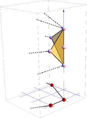
Figure 1: Vertical projection from the 3d toric diagram of $Y_{4}$ to the 2d toric diagram of $Y_{3}$. The three aligned points give rise to two D6-branes.

In our example, the fact that two adjacent external points in the 3d toric diagram project to the same point (which is then necessarily strictly external) in the 2d toric diagram, implies the presence of a D6-brane wrapping a toric divisor of the CY₃ in type IIA (spanning the spacetime $\mathbb{R}^{2,1}$ and localized at $r_{0}=0$). The toric divisor is specified by the projected point. More generally, if the 3d toric diagram has a collection of $h+1$ aligned adjacent external points $(1,x,y,z_{j})$ with $z_{j}=z$, $z+1$, …, $z+h$, and we reduce along the $U(1)_{M}$ cycle $(0,0,0,1)$, all $h+1$ points project down to the same strictly external point in the 2d toric diagram and give rise to $h$ coincident D6-branes wrapping a toric divisor of the CY₃ (see Figure 1).

Along the D6-branes lives a $U(h)$ gauge theory, which by the AdS/CFT map corresponds to a $U(h)$ global symmetry on the boundary. We could then expect the boundary theory to admit a description in which such a symmetry is manifest. The same conclusion can be reached in M-theory: $h+1$ adjacent external points in the 3d toric diagram indicate $h$ KK monopoles in $Y_{4}$ (a multi-Taub-NUT geometry), whose complex structure is locally $\mathbb{C}^{2}\times\mathbb{C}^{2}/\mathbb{Z}_{h}$; the $A_{h-1}$ singularity carries $SU(h)$ gauge fields, besides the $U(1)$ gauge field from the KK reduction of the M-theory potential $C_{3}$. More precisely, in the near core limit the latter $U(1)$ KK mode is non-normalizable – correspondingly in the dual theory the diagonal $U(1)$ in $U(h)$ is actually gauged.

2.1 CY₄ as a $U(1)$ fibration

Let us explain how to rewrite a toric CY $d$-fold as a (possibly singular) $U(1)$ fibration over a manifold, which in turn is the fibration of a toric CY $(d-1)$-fold along a real line, with Kähler moduli that vary linearly along the line. In the first part, we follow the exposition in [17].

Consider a toric CY $d$-fold, realized as the moduli space of a gauged linear sigma-model (GLSM). There are $N+d$ chiral superfields $\phi_{s}$ with $s=1,\dots,N+d$, and $N$ $U(1)$ gauge groups with integer charges $Q^{a}_{s}$ (of maximal rank) with $a=1,\dots,N$. The CY condition is $\sum_{s}Q^{a}_{s}=0$ for all $a$. The number $N+d$ of fields can be taken to be equal to the number of dots in the $(d-1)$-dimensional toric diagram. Then the charge matrix $Q^{a}_{s}$ encodes the $N$ linear relations $\sum_{s}Q^{a}_{s}\,\vec{v}_{s}=0$ between the vectors $\{\vec{v}_{s}\}$ in the toric fan. The CY $Y_{d}$ is simply the Kähler quotient $\mathbb{C}^{N+d}//U(1)^{N}$, which corresponds to imposing the moment map (D-term) equations

$$\sum\nolimits_{s}Q^{a}_{s}\,|\phi_{s}|^{2}=r^{a}$$ (2.1)

and quotienting by the gauge group

$$\phi_{s}\;\to\;e^{i\sum_{a}\lambda_{a}Q^{a}_{s}}\,\phi_{s}\;.$$ (2.2)

The moment map (or FI) parameters $r^{a}$ are the resolution parameters of $Y_{d}$. We will be mainly interested in the conical case $r^{a}=0$. Moreover, for each $a$ the charges $Q^{a}_{s}$ can be taken coprime without loss of generality.

To exhibit the fibered structure, we add the complex variable $r_{0}+i\theta_{0}$ and choose a set of charges $Q^{0}_{s}$ satisfying the CY condition $\sum_{s}Q^{0}_{s}=0$. Then we impose one more equation and divide by one more gauge symmetry:

$$\sum\nolimits_{s}Q^{0}_{s}\,|\phi_{s}|^{2}=r_{0}\;;\qquad\qquad\theta_{0}\;\to\;\theta_{0}+\lambda\;,\qquad\phi_{s}\;\to\;e^{i\lambda\,Q^{0}_{s}}\,\phi_{s}\;.$$ (2.3)

It is easy to check that the manifold is the same as before: using (2.3) $r_{0}$ can be eliminated while $\theta_{0}$ can be gauged away (without leaving any residual gauge transformation).

On the other hand, we can fix $r_{0}$ and think of $\theta_{0}$ as a $U(1)$ fibration. The base manifold $Y_{d-1}$ is then the Kähler quotient $\mathbb{C}^{N+d}//U(1)^{N+1}$:

$$\sum\nolimits_{s}Q^{0}_{s}\,|\phi_{s}|^{2}=r_{0}\;,\qquad\qquad\sum\nolimits_{s}Q^{a}_{s}\,|\phi_{s}|^{2}=r^{a}\qquad\forall\,a=1,\dots,N\;,$$ (2.4)

modded out by

$$\phi_{s}\;\to\;e^{i\lambda\,Q^{0}_{s}\;+\;i\sum_{a}\lambda_{a}Q^{a}_{s}}\,\phi_{s}\;.$$ (2.5)

$Y_{d-1}$ is toric and Calabi-Yau. Moreover, $Y_{d-1}$ is fibered over the real line $r_{0}$, with a particular combination of the resolution parameters (set by $Q^{0}_{s}$) varying linearly with $r_{0}$. The tip of $Y_{d}$ is at $r_{0}=0$.

Projecting the toric diagram.

Given the set of charges $Q^{a}_{s}$, the toric fan of $Y_{d}$ is given by $N+d$ primitive vectors $\{\vec{v}_{s}\}$ in $\mathbb{Z}^{d}$ which solve the $N$ linear conditions $\sum_{s}Q^{a}_{s}\,\vec{v}_{s}=0$ for all $a=1,\dots,N$. We can collect the vectors as columns of a matrix $(G_{K})^{i}_{s}$, with $i=1,\dots,d$, of maximal rank. Then

$$Q^{a}_{s}\,(G_{K}^{T})^{s}_{i}=0$$ (2.6)

and the rows of $G_{K}$ span the kernel of $Q^{a}_{s}$ as a map from $\mathbb{R}^{N+d}$ to $\mathbb{R}^{N}$. We can use a transformation of $SL(d,\mathbb{Z})$ to map the vectors to $\vec{v}_{s}=(1,\vec{w}_{s})$. The same equation can be used to obtain the charges of a GLSM, given the matrix $G_{K}$ of all vectors in the toric fan.

The toric diagram of $Y_{d-1}$ can be obtained in the same way. We add the extra condition $\sum_{s}Q_{s}^{0}\,\vec{v}_{s}=0$. The vectors $\vec{v}_{s}$ do not satisfy it, because the rows of $(G_{K})^{i}_{s}$ are linearly independent. In order to satisfy the extra relation, we must project the vectors on a hyperplane in such a way that the linear combination

$$\vec{v}_{M}\equiv\text{primitive }\sum\nolimits_{s}Q^{0}_{s}\,\vec{v}_{s}$$ (2.7)

vanishes, that is a hyperplane orthogonal to $\vec{v}_{M}$. Notice that the CY condition on $Q^{0}_{s}$ plus the particular chosen frame $\vec{v}_{s}=(1,\vec{w}_{s})$ assures that $\vec{v}_{M}=(0,\vec{w}_{M})$. To make the projection clearer, we can perform an $SL(d-1,\mathbb{Z})$ transformation that maps $\vec{v}_{M}$ to $(0,\dots,0,1)$, and changes the toric diagram of $Y_{d}$ accordingly. Then the toric diagram of $Y_{d-1}$ is obtained from the one of $Y_{d}$ with the “vertical” projection that forgets the last component (Figure 1).

Fixed points.

The reduction $Y_{d-1}=Y_{d}//U(1)_{M}$ can always be done. However, whenever the $U(1)_{M}$ fiber degenerates, we should expect some extra object or singularity in the type IIA background, on top of any possible geometric toric singularity (even non-isolated) of $Y_{d-1}$.

A first class of singularities arises from loci where the fiber $U(1)_{M}$ shrinks:

• each strictly external dot $\vec{v}_{s}$ in the $(d-1)$-dimensional toric diagram of $Y_{d}$ is a conical toric divisor (complex codimension one) where the circle $\vec{v}_{s}$ shrinks;

• each external edge $v_{sr}$ connecting two adjacent dots $\vec{v}_{s}$ and $\vec{v}_{r}$ is a conical codimension 2 surface where the span in $U(1)^{d}$ of the two circles shrinks;

• each external polyhedron $v_{s_{1}\dots s_{n}}$ of dimension $n-1$ constructed between the strictly external dots $\vec{v}_{s_{1}},\dots,\vec{v}_{s_{n}}$ is a conical codimension $n$ surface where the span in $U(1)^{d}$ of the $n$ circles shrinks.

In order to have a non-singular Kähler quotient for the projection, we should make sure that the circle $\vec{v}_{M}$ is not contained in any of the spans above (the first case is automatically excluded). Practically, we require $\vec{w}_{M}$ not to be parallel to any external sub-object in the convex polyhedron of the $(d-1)$-dimensional toric diagram. We stress that we are not worried about singularities in the quotient $Y_{d-1}$, but rather about degenerations of the fiber.

There is a second class of possible singularities, where the $U(1)_{M}$ fiber degenerates to $U(1)/\mathbb{Z}_{p}$ for some $p$. This happens if some of the charges in $Q^{0}_{s}$ have modulus larger than 1. In this case, there could be a conical surface where the fiber $U(1)_{M}$ degenerates: we have to make sure that the only point where this happens is the tip of $Y_{d}$.

The case of CY₄.

Specializing to the case of interest – $Y_{4}$ and $Y_{3}=Y_{4}//U(1)_{M}$ –, whenever none of the singularities above arises in the quotienting, we are sure that the reduction of M-theory on $Y_{4}$ along $U(1)_{M}$ gives a pure IIA background (to which the arguments in [17] can be applied), without extra objects on top of it.

In particular, we should make sure that: 1) there are no external edges in the 3d toric diagram parallel to $\vec{w}_{M}$; 2) there are no external faces parallel to $\vec{w}_{M}$; 3) once $\vec{w}_{M}$ is expressed as an integer sum of the $\vec{w}_{s}$ in the 3d toric diagram, if some coefficients have modulus larger than 1, the fiber does not degenerate outside the tip of $Y_{4}$.

On the contrary, whenever the fiber degenerates, we should expect some extra objects in type IIA that have to be taken into account. In this paper we study what happens if the fiber shrinks on a complex codimension-two submanifold of the four-fold (giving rise to D6-branes). The other cases deserve a separate study.

2.2 IIA background as a CY₃ fibration with D6-branes

The symplectic reduction of $Y_{4}$ to a CY₃ is useful because it allows to exploit all the powerful techniques available for D3-branes probing toric singularities, to get information about the field theory. Given a toric CY₃ singularity in type IIB and $N$ D3-branes probing it, the dual SCFT in 3+1 dimensions can be generically found with the algorithm in [48] (see also [49]). As explained in [17], we can consider the same CY₃ singularity in type IIA and probe it with D2-branes: the dual theory is the same quiver (with same superpotential) as before, but in 2+1 dimensions. We can further include RR fluxes and fiber the CY₃ over a real line (in an $\mathcal{N}=2$ supersymmetric way). This corresponds to switching on $\mathcal{N}=2$ Chern-Simons couplings in the Yang-Mills (YM) quiver gauge theory. Conversely, whenever the symplectic reduction CY${}_{4}//U(1)_{M}$ is regular (the fiber $U(1)_{M}$ nowhere degenerates), the procedure allows to obtain a CS quiver theory which reproduces the CY₄ in its moduli space. The relation between the $CY_{4}$ geometric moduli space of a 3d quiver CS theory and the $CY_{3}=CY_{4}//U(1)_{M}$ mesonic moduli space of a 4d gauge theory with the same quiver and superpotential was first pointed out in [6, 7, 8].

We aim to extend the correspondence to cases in which the Kähler quotient has complex dimension-two degeneration loci. To begin with, let us understand what the toric divisors of $Y_{3}$ correspond to. Each strictly external point $\vec{p}$ in the 2d toric diagram corresponds to a toric divisor, to which is associated a collection of $Q$ bifundamental fields $\{X_{\eta}\}_{\eta=1,\dots,Q}$ in the quiver theory, that have the same charges under all global (but not gauge) symmetries. The number $Q$ is given by [50]

$$Q=\left|\det\begin{pmatrix}\Delta x&\Delta y\\ \Delta x^{\prime}&\Delta y^{\prime}\end{pmatrix}\right|\;,$$ (2.8)

where $(\Delta x,\Delta y)$ is the vector connecting the strictly external point $\vec{p}$ to the next strictly external point along the perimeter, while $(\Delta x^{\prime},\Delta y^{\prime})$ is the vector connecting $\vec{p}$ to the previous strictly external point. A time-filling D3-brane wrapped on the 3-cycle which is the radial section of the toric divisor (such embedding is supersymmetric) corresponds to a dibaryonic operator $X_{\eta}^{N}$ [51, 44, 52]. Since the 3-cycle has the topology of a Lens space with fundamental group $\mathbb{Z}_{Q}$ [44], the D3-branes admit a $\mathbb{Z}_{Q}$ flat connection resulting in $Q$ degenerate vacua. They correspond to the $Q$ different dibaryonic operators $\{X_{\eta}^{N}\}$. An easy way to identify the set of fields is through perfect matchings (that we review in Appendix A) in the brane tiling construction [53, 54, 55, 49].

Instead of wrapping a D3-brane on a radial section, one can wrap $h$ spacetime-filling D7-branes on the whole toric divisor (this problem has been considered, e.g., in [56, 57, 58, 59, 60]). They introduce a $U(h)$ global symmetry in the field theory, and $h$ flavors of chiral fields $p_{\eta}$, $q_{\eta}$ coupled to one of the bifundamental fields $X_{\eta}$ through the superpotential term $W=p_{\eta}X_{\eta}q_{\eta}$. A $\mathbb{Z}_{Q}$ connection, flat everywhere but at the tip, can be specified on the D7-branes to distinguish which bifundamental is flavored.

The same discussion holds in type IIA: D6-branes wrapping toric divisors of the CY₃ provide chiral flavors to the quiver gauge theory on D2-branes at the tip. Each stack of $h$ D6-branes introduces a $U(h)$ flavor group (this is not always the case: we will be more precise in Section 5) and flavor chiral multiplets $p_{\hat{k}i}$, $q_{j\hat{k}}$ coupled to a bifundamental $X_{ij}$ through a superpotential term

$$W=\operatorname{Tr}p_{\hat{k}i}X_{ij}q_{j\hat{k}}\;.$$ (2.9)

Here $\hat{k}$ stands for a flavor group, $i,j$ for gauge groups and fields are in the fundamental (anti-fundamental) of the first (second) index; all indices are contracted. We will jump between the notations $X_{a}$ and $X_{ij}$ for bifundamental fields. The field $X_{ij}$ is determined as explained above.

The D6-branes are localized along $\mathbb{R}$: reducing the cone $Y_{4}$ their position is $r_{0}=0$. More generally, the position along $r_{0}$ corresponds to a real mass for the quarks in field theory, and to a partial resolution (or Kähler) parameter in M-theory (see Section 5.1). Since D6-branes, possibly with worldvolume flux, are sources for RR fields, the 2- and 4-form fluxes on 2- and 4-cycles vanishing at the CY₃ singularity jump at $r_{0}$:

$$\delta\int_{\mathcal{C}_{2}}F_{2}=\#(\mathcal{C}_{2},D6)\;,\qquad\qquad\delta\int_{\mathcal{C}_{4}}F_{4}=\#(\mathcal{C}_{4},D6,\mathcal{C}_{4}^{(F_{\mathrm{wv}})})\;,$$ (2.10)

where the jump depends on the intersection on $Y_{3}$ between the cycles, the divisor and the cycle representing the worldvolume flux. This means that moving the D6’s to the left or to the right of the D2-branes, the CS levels must jump as well. We will study this in detail.

Summarizing, whenever the $U(1)_{M}$ action has codimension-two fixed loci which descend in type IIA to D6-branes wrapping divisors of the CY₃, the field theory derived using the CY₃ singularity is actually flavored.

We conclude this section with some comments. Two important differences between chiral flavors in $AdS_{5}/CFT_{4}$ and in $AdS_{4}/CFT_{3}$ must be borne in mind. Firstly, in 4d gauge theories chiral flavors are constrained by gauge anomaly cancelation, whereas in 3d such a constraint does not exist. The dual statement is that D7-branes wrapping divisors are constrained by RR $C_{0}$ tadpole cancelation, whilst D6-branes are not because the RR $F_{2}$ flux can escape to infinity along the transverse non-compact real line. The number of fundamental minus anti-fundamental fields for a gauge group in 3d need not vanish: if it is odd, the parity anomaly requires the presence of half-integral CS levels [61, 62, 63]. Secondly, in general the addition of flavors to an $AdS_{5}/CFT_{4}$ pair breaks conformal invariance and the RG flows leads the theory to a fixed point which is outside the validity of supergravity [58] (the dual statement is that D7-branes force the dilaton to run towards $-\infty$ at the tip). Flavoring $AdS_{4}/CFT_{3}$ pairs, the theory still flows to an interacting fixed point which however in many examples [27, 28, 29, 64, 65] (and in the ones of this paper too) is still described by type IIA/M-theory.

In the following, we will focus on the Abelian case: we will consider a single M2/D2-brane and the corresponding quiver theory will have $U(1)$ gauge groups. One expects the low energy field theory on a stack of $N$ M2/D2-branes to be described by the same quiver with $U(N)$ gauge groups, and the geometric moduli space to be the symmetric product of $N$ copies of $Y_{4}$. We leave the non-Abelian extension for the future.

3 Flavoring Chern-Simons-matter theories
A bottom-up perspective

In the rest of this paper we turn to a bottom-up perspective. We start with a generic toric CY₄ geometry and a regular (as described in Section 2.1) IIA reduction along $U(1)_{M}$, such that the Chern-Simons-matter theory dual to M2-branes probing $Y_{4}$ can be read off [17]. Then we study the effect of chirally flavoring such a theory in a very general way, and in particular we study how the flavoring deforms the moduli space of the quiver theory. Alternatively, we can start with a toric CY₃ geometry and its dual quiver theory (which in 3+1 dimensions is the theory dual to D3-branes probing $Y_{3}$), add to it generic $\mathcal{N}=2$ Chern-Simons couplings (which corresponds to fibering $Y_{3}$ over $\mathbb{R}$ and adding RR fluxes) and flavors (D6-branes), and study what is the resulting CY₄ geometry seen by M2-branes.

To begin with, let us specify the flavoring procedure. The starting point is an $\mathcal{N}=2$ quiver Chern-Simons theory in 2+1 dimensions. The matter fields are chiral multiplets $X_{a}$ in the adjoint or bifundamental representation, and we restrict ourselves to the Abelian case. Then we introduce $B$ families of flavor chiral multiplets $(p_{\alpha},q_{\alpha})$, each coupled to a matter field $X_{\alpha}$ via the superpotential

$$W=W_{0}+\sum\nolimits_{\alpha}p_{\alpha}X_{\alpha}q_{\alpha}\;.$$ (3.1)

Here $p_{\alpha}$ ($q_{\alpha}$) transform in the anti-fundamental (fundamental) of the gauge group under which $X_{\alpha}$ is in the fundamental (anti-fundamental). Each pair $(p_{\alpha},q_{\alpha})$ really represents $h_{\alpha}$ fields, and introduces a $U(h_{\alpha})$ flavor symmetry.

We could be more general and couple a flavor pair to a bifundamental operator $\mathcal{O}_{\alpha}=\prod_{\beta=1}^{n}X_{\beta}$ constructed from a string of matter fields $X_{\beta}$. This is equivalent to coupling each of the $X_{\beta}$ to its own flavor pair $(p_{\beta},q_{\beta})$, and then introducing complex masses

$$W=W_{0}+\sum_{\beta=1}^{n}p_{\beta}X_{\beta}q_{\beta}+\sum_{\beta=1}^{n-1}m_{\beta}\,p_{\beta+1}q_{\beta}\;.$$ (3.2)

Integrating out the massive fields, we flavor the operator $\mathcal{O}_{\alpha}$ (see Section 5.2).

Every time we introduce two new flavor fields $(p,q)$ coupled to $X_{\alpha}$, the parity anomaly [61, 62, 63] requires to shift two CS levels as

$$\delta k_{i}=\pm\frac{1}{2}\,g_{i}[X_{\alpha}]\;,$$ (3.3)

$g_{i}$ being the gauge charges. The sign is a choice of theory. If we add $h_{\alpha}$ flavors $(p_{\alpha},q_{\alpha})$, we choose sign $h_{\alpha}$ times, so that the shift

$$\delta k_{i}=\Big{(}\frac{h_{\alpha}}{2}-\gamma_{\alpha}\Big{)}\,g_{i}[X_{\alpha}]$$ (3.4)

is parametrized by an integer $\gamma_{\alpha}$ with $0\leq\gamma_{\alpha}\leq h_{\alpha}$.

The reason for this is that gauge invariance requires

$$k_{i}+\frac{1}{2}\sum\nolimits_{\psi}\big{(}g_{i}[\psi]\big{)}^{2}\,\in\mathbb{Z}\;,$$ (3.5)

where the sum runs over all fermions charged under the $i$-th gauge group. When the second term is half-integral, the fermion determinant is multiplied by $(-1)$ under certain gauge transformations, and the lack of gauge invariance of the CS terms cures it. In our setup the gauge charges of flavors are $g_{i}=\pm 1$, so consistency requires that each addition of two flavor fields is accompanied by a half-integral opposite shift of two CS levels (unless $X_{\alpha}$ is in the adjoint).

We can proceed in the opposite way and integrate the flavors out. In 2+1 dimensions it is possible to give real mass $\tilde{m}$ to a chiral multiplet $Z$ through the Lagrangian term [66, 67]

$$\int d^{4}\theta\,Z^{\dagger}e^{\tilde{m}\theta\bar{\theta}}Z\;.$$ (3.6)

To give real masses to the flavors, we promote the $U(h)$ flavor symmetry to a background gauge symmetry; then a VEV $\langle\sigma_{F}\rangle$ for the real adjoint background scalar field $\sigma_{F}$ in the $U(h)$ vector multiplet provides real masses to all flavors charged under $U(h)$. After diagonalization of $\langle\sigma_{F}\rangle$ by a flavor rotation, each flavor of charge $q_{\psi}$ acquires a real mass $M_{\psi}=q_{\psi}\langle\sigma_{F}\rangle$. When integrating out massive fermions $\{\psi\}$, the CS levels $k_{i}$ are shifted by one-loop diagrams as

$$k_{i}\to k_{i}+\frac{1}{2}\sum\nolimits_{\psi}\big{(}g_{i}[\psi]\big{)}^{2}\operatorname{Sgn}(M_{\psi})\;.$$ (3.7)

Integrating out just two flavor fields $(p,q)$, $M_{p}=\langle\sigma_{F}\rangle$ and $M_{q}=-\langle\sigma_{F}\rangle$; we can then write $\delta k_{i}=\frac{1}{2}g_{i}[X_{\alpha}]\,\operatorname{Sgn}(\langle\sigma_{F}\rangle)$. The choice of $\operatorname{Sgn}(\langle\sigma_{F}\rangle)$ corresponds to the choice of sign in (3.3): a choice of positive (negative) sign in (3.3) is undone by $\langle\sigma_{F}\rangle<0$ ($\langle\sigma_{F}\rangle>0$).

In the next subsection we compute the effect of flavors on monopole operators, while in Section 4 we study the moduli space of the flavored theories.

3.1 Monopole operators and flavors

A fundamental rôle in the study of the quantum moduli space of the flavored theories is played by monopole operators [34, 35, 36, 37, 38, 39, 40, 41]: in the Euclidean theory, their insertion creates quantized flux in a $U(1)$ subgroup of the gauge group through a sphere surrounding the insertion point. In radial quantization, they correspond to states with flux on $S^{2}$. For a $U(1)$ gauge group:

$$\frac{1}{2\pi}\int_{S^{2}}F=n\;.$$ (3.8)

In a Chern-Simons theory, monopole operators pick up an electric charge since

$$S\;\supset\;\frac{k}{4\pi}\int A\wedge dA=k\,n\int A_{0}\,dt\;,$$ (3.9)

where $k$ is the Chern-Simons level. In a Chern-Simons-matter theory, fermionic matter fields can correct these charges from 1-loop diagrams. A special rôle is played by “diagonal” monopole operators, that we will denote $T^{(n)}$ with $n\in\mathbb{Z}$: they have the same flux $n$ along all $U(1)$ gauge groups in the quiver. They pick up electric charges $(nk_{1},\dots,nk_{G})$ under $U(1)^{G}$, where $G$ is the number of gauge factors and $k_{i}$ are the CS levels. They were studied in detail in [41] and shown to be BPS (after having been dressed by scalar modes) in the ABJM theory [1]; we expect them to be BPS in generic $\mathcal{N}=2$ theories describing M2-branes on CY₄, since they correspond to modes of eleven-dimensional supergravity in short multiplets.

The monopole operators $T^{(n)}$ can acquire a charge under any $U(1)$ symmetry of the theory, both global and gauged, from quantum corrections [37, 38, 39, 41]. In the case of global symmetries the charge comes entirely from fermionic modes, while in the case of gauge symmetries the quantum contribution sum up with (3.9). The quantum correction (in the Abelian case) to the charge $Q$ from fermionic modes is

$$\delta Q[T^{(n)}]=-\frac{|n|}{2}\,\sum\nolimits_{\psi}Q[\psi]\;,$$ (3.10)

where we sum over all fermions $\psi$ in the theory. Notice that only fermions in chiral representations contribute. The result is proportional to the mixed $Q$-gravitational anomaly that the same theory would have in 3+1 dimensions.

Formula (3.10) implies that in Chern-Simons quiver theories satisfying the toric condition, diagonal monopole charges do not receive any quantum correction. Quiver theories have matter chiral multiplets in the adjoint and bifundamental representation only; the toric condition is that all gauge ranks are the same (here 1), each matter field appears in the superpotential in exactly two monomials, and the number $G$ of gauge groups plus the number $P$ of monomials in the superpotential equals the number $E$ of matter fields. Let $Q$ be a non-R global or gauge symmetry: each monomial $W_{\mu}$ in the superpotential must have vanishing charge. Summing over all monomials: $2\sum_{\psi}Q[\psi]=2\sum_{a}Q[X_{a}]=\sum_{\mu}\sum_{a\in\mu}Q[X_{a}]=0$, where $X_{a}$ are all matter fields, and gaugini must be chargeless. In the case of the R-symmetry, each monomial $W_{\mu}$ must have R-charge 2, so that: $2\sum_{\psi}R[\psi]=2G+2\sum_{a}R[\psi_{a}]=2G-2E+2\sum_{a}R[X_{a}]=2G-2E+2P=0$, where we used the fact that gaugini have R-charge 1.

Therefore, let us start with a quiver theory in which the monopole fields $T^{(n)}$ have only gauge charges $(nk_{1},\dots,nk_{G})$. Then we flavor the theory as in (3.1): we couple a set of flavor pairs $(p_{\alpha},q_{\alpha})$, each in number $h_{\alpha}$, to some bifundamental operators $X_{\alpha}$ in the quiver, constructed as products of bifundamental fields, via

$$W=W_{0}+\sum\nolimits_{\alpha}p_{\alpha}X_{\alpha}q_{\alpha}\;.$$ (3.11)

We are interested in the charges induced on the monopole operators by flavors. Let us start with non-R symmetries. First, there are the new flavor symmetries $U(h_{\alpha})$ of which $p_{\alpha}$ and $q_{\alpha}$ are in conjugate representations, so that the diagonal monopole operators cannot get a charge under $U(h_{\alpha})$. Next, for any $U(1)$ flavor symmetry of $W_{0}$ under which $X_{\alpha}$ has charge $Q_{\alpha}$, $(qp)_{\alpha}$ must have charge $-Q_{\alpha}$. Then, according to (3.10), the diagonal monopoles pick up a charge

$$Q[T^{(n)}]=\frac{|n|}{2}\sum\nolimits_{\alpha}h_{\alpha}\,Q[X_{\alpha}]$$ (3.12)

in the flavored quiver. In the case of gauge charges, the contribution from fermions has to be summed with the contribution from Chern-Simons couplings:

$$g_{i}[T^{(n)}]=nk_{i}+\frac{|n|}{2}\sum\nolimits_{\alpha}h_{\alpha}\,g_{i}[X_{\alpha}]\;,$$ (3.13)

where $g_{i}$ are the gauge charges under $U(1)^{G}$. Eventually, consider the R-symmetry: $R[p_{\alpha}]+R[q_{\alpha}]=2-R[X_{\alpha}]$ at the IR fixed point, so that the monopoles get an R-charge

$$R[T^{(n)}]=-\frac{|n|}{2}\sum\nolimits_{\alpha}h_{\alpha}\,\big{(}R[\psi_{p_{\alpha}}]+R[\psi_{q_{\alpha}}]\big{)}=\frac{|n|}{2}\sum\nolimits_{\alpha}h_{\alpha}\,R[X_{\alpha}]\;.$$ (3.14)

These charges allow us to conjecture the following holomorphic quantum relation:

$$T^{(n)}\,T^{(-n)}=\Big{(}\prod\nolimits_{\alpha}X_{\alpha}^{h_{\alpha}}\Big{)}^{|n|}\;,$$ (3.15)

which is consistent with all manifest symmetries in the action. This is understood as an operator statement: the equation must be multiplied on both sides by the necessary fields to form gauge-invariant operators. In Section 4 we show that in the usual unflavored case (where quantum corrections seem not to play a rôle) the relation $T^{(n)}T^{(-n)}=1$ can be inferred from the form of the moduli space. Moreover, (3.15) is analogous to the quantum relation which appeared in the $\mathcal{N}=3$ setup of [27] (see also [38]), and we will show that it reproduces the CY₄ moduli spaces as expected from the M-theory reduction, as we also check in several examples in Section 6. In the following we will use the notation

$$T^{(1)}\equiv T\;,\qquad T^{(-1)}\equiv\tilde{T}\;,$$ (3.16)

for the simplest diagonal monopole operators.

4 Moduli space of flavored quivers

4.1 Unflavored quivers and monopoles

The moduli space of any (unflavored) $\mathcal{N}=2$ Chern-Simons quiver theory was worked out in [7]. Let us review the analysis here, and show how the monopole operators $T$, $\tilde{T}$ can be included at the classical level. We focus on the Abelian case, and impose the further condition $\sum k_{i}=0$.

The F-term equations $\partial W/\partial X_{a}=0$, where $X_{a}$ are all the chiral superfields in the quiver and $a=1,\dots,M$, define an algebraic variety

$$\mathcal{Z}=\{X_{a}\;|\;dW=0\}\subset\mathbb{C}^{M}\;.$$ (4.1)

This is exactly the same as in the corresponding quiver theory in 3+1 dimensions. The D-term equations are

$$\mathcal{D}_{i}=\frac{k_{i}\sigma_{i}}{2\pi}\qquad\forall\,i\qquad\text{ and }\qquad|X_{a}|^{2}\,\Big{(}\sum\nolimits_{i}g_{i}[X_{a}]\,\sigma_{i}\Big{)}^{2}=0\qquad\forall\,a\;,$$ (4.2)

where $\mathcal{D}_{i}$ with $i=1,\dots,G$ are the D-terms expressed in terms of the scalars in chiral multiplets

$$\mathcal{D}_{i}\equiv\sum\nolimits_{a}g_{i}[X_{a}]\,|X_{a}|^{2}\;,$$ (4.3)

while $\sigma_{i}$ are the real scalars in the $\mathcal{N}=2$ vector multiplets. We focus on the particular branch $\sigma_{1}=\dots=\sigma_{G}\equiv\sigma$, which is a CY four-fold [7]. The second set of equations in (4.2) is then automatically solved. We can rewrite the first set as

$$\sum\nolimits_{i}c_{i}\,\mathcal{D}_{i}=0\qquad\forall\,\{c_{i}\}\text{ such that }\sum\nolimits_{i}c_{i}k_{i}=0\;.$$ (4.4)

If $k_{i}$ are not all vanishing, these are $G-2$ independent equations (the equation with $c_{i}=1$ is trivial, as follows from (4.3)). The scalar $\sigma$ can be eliminated by

$$\frac{\sigma}{2\pi}=\sum\nolimits_{i}\frac{k_{i}}{|k|^{2}}\,\mathcal{D}_{i}\;,$$ (4.5)

where $|k|^{2}=\sum_{i}k_{i}^{2}$.

Naively, one would divide by $U(1)^{G-1}$ gauge transformations (no scalar transforms under the diagonal $U(1)_{\mathrm{diag}}$), but this would give an odd dimensional space. In fact, the diagonal photon $A_{\mathrm{diag}}\equiv\sum_{i}A_{i}$ is only coupled to the other photons via a $bf$ term, whilst it is not coupled to any matter current. Hence it can be dualized into a scalar $\tau$, which is invariant under $U(1)_{\mathrm{diag}}$ but transforms under the remaining group,

$$A_{i}\;\to\;A_{i}+d\theta_{i}\;,\qquad\qquad\tau\;\to\;\tau+\frac{1}{G}\sum\nolimits_{i}k_{i}\,\theta_{i}\;.$$ (4.6)

We can use a gauge transformation to gauge $\tau$ away: this leaves us with $U(1)^{G-2}$ gauge transformations (the ones with $\sum k_{i}\theta_{i}=0$), which precisely correspond to the $G-2$ D-term equations in (4.4), plus a residual discrete group from the gauge fixing of $\tau$. On the branch we consider, in Euclidean signature the energy of the vacuum vanishes when $A_{1}=\dots=A_{G}$ (which is a diagonal flux), hence the quantization $\frac{1}{2\pi}\int dA_{\mathrm{diag}}\in G\,\mathbb{Z}$ [7], which implies that $\tau$ has period $2\pi/G$. The gauge fixing of $\tau$ leaves a residual $\mathbb{Z}_{q}$ symmetry, where $q=\gcd\{k_{i}\}$, to divide by. As a result, the moduli space is a $\mathbb{Z}_{q}$ quotient of the Kähler quotient:

$$\mathcal{M}=(\mathcal{Z}//U(1)^{G-2})/\mathbb{Z}_{q}\;.$$ (4.7)

Including monopole operators.

We can describe the same moduli space in a slightly different way. Instead of gauge fixing $\tau$, we keep it in the description of the moduli space. Given the periodicity of $\tau$, we can construct the two complex fields

$$T=\rho\,e^{iG\,\tau}\;,\qquad\qquad\tilde{T}=\tilde{\rho}\,e^{-iG\,\tau}\;,$$ (4.8)

where their dimensionless moduli $\rho$ and $\tilde{\rho}$ are not specified yet. The gauge transformations are

$$T\;\to\;e^{i\sum k_{i}\theta_{i}}\,T\;,\qquad\qquad\tilde{T}\;\to\;e^{-i\sum k_{i}\theta_{i}}\,\tilde{T}\;,$$ (4.9)

so that their gauge charges are $\pm(k_{1},\dots,k_{G})$ respectively. Keeping $T$, $\tilde{T}$ in the description, we will have to divide by the full gauge group $U(1)^{G}$ (still nothing is charged under $U(1)_{\mathrm{diag}}$). We can rewrite the D-term equations (4.4) and (4.5) as

$$0=\tilde{\mathcal{D}}_{i}=k_{i}\,g^{2}\,|T|^{2}-k_{i}\,g^{2}\,|\tilde{T}|^{2}+\mathcal{D}_{i}\qquad\forall\,i$$ (4.10)

with the extra complex constraint

$$T\tilde{T}=1\;,$$ (4.11)

where $\tilde{\mathcal{D}}_{i}$ are “improved D-terms”. Here $g^{2}$ is some mass scale, discussed below. The improved D-term equations can be thought of as arising in the presence of extra chiral fields $T$, $\tilde{T}$ with charges $\pm(k_{1},\dots,k_{G})$.

The equivalence works as follows:

$$0 =\sum_{i}c_{i}\tilde{\mathcal{D}}_{i}=\sum_{i}c_{i}\mathcal{D}_{i}\qquad\qquad\forall\,\{c_{i}\}\text{ s.t. }\sum_{i}c_{i}k_{i}=0$$ (4.12)

$$0 =\sum_{i}\frac{k_{i}}{|k|^{2}}\,\tilde{\mathcal{D}}_{i}=g^{2}|T|^{2}-g^{2}|\tilde{T}|^{2}+\sum_{i}\frac{k_{i}}{|k|^{2}}\,\mathcal{D}_{i}\;.$$

The first set is exactly (4.4). The second equation is equivalent to (4.5) if we express $\rho$ and $\tilde{\rho}$ in terms of $\sigma$ through the equations (4.11) and

$$|T|^{2}-|\tilde{T}|^{2}+\frac{\sigma}{2\pi g^{2}}=0.$$ (4.13)

These two equations have one and only one solution in terms of $\sigma$.

As a result, the same moduli space can be obtained by adding $T$, $\tilde{T}$ to the set $\{X_{a}\}$ of chiral fields, adding (4.11) to the set of classical F-term relations derived from the superpotential, and dividing by the full gauge group $U(1)^{G}$. Rephrasing, we start with a larger algebraic variety

$$\tilde{\mathcal{Z}}=\{X_{a},T,\tilde{T}\;|\;dW=0,\,T\tilde{T}=1\}\subset\mathbb{C}^{M+2}\;,$$ (4.14)

and construct the geometric moduli space as the Kähler quotient

$$\mathcal{M}=\tilde{\mathcal{Z}}//U(1)^{G}\;.$$ (4.15)

It is natural to associate $T$ and $\tilde{T}$ with the monopole operators. In fact, following [67], it is natural to combine the vector multiplet scalar $\sigma$ and the scalar dual to the photon in a chiral multiplet. The mass scale $g^{2}$ does not affect the moduli space, and we can use the coupling of the diagonal photon $A_{\mathrm{diag}}$ in a YM-CS UV completion of the theory. The relation (4.11) is a particular case of the quantum relation (3.15): we see that in the unflavored case it appears at the classical level, in the parametrization of the moduli space. In fact $T$ and $\tilde{T}$ are necessary to parametrize the moduli space with operators invariant under the full $U(1)^{G}$ gauge group.

The toric case.

In case the CS-matter quiver theory is a brane tiling [53, 54, 55, 49], this branch of the moduli space is a toric CY₄. A brane tiling (more details in Appendix A) is a bipartite graph on the torus which encodes both the matter content (the quiver) and the superpotential of the gauge theory, and imposes particular constraints on them. Brane tilings describe the quiver gauge theories dual to D3-branes probing toric CY₃ singularities and so, by the construction of [17] reviewed in Section 2, they become relevant for M2-branes probing toric CY₄ singularities as well. In this case, the brane tiling can be refined to include the Chern-Simons levels $k_{i}$ (with the constraint $\sum_{i}k_{i}=0$). One assigns an integer $n_{ij}$ to each bifundamental field $X_{ij}$ – the CS levels are then defined to be $k_{i}=\sum_{j}(n_{ij}-n_{ji})$ [9, 10].

The geometric moduli space of a CS-matter brane tiling theory can be easily computed with the Kasteleyn matrix algorithm, that we review in Appendix A. The algorithm furnishes the following output:

• A set of fields $t_{\rho}$, called perfect matchings, in terms of which the bifundamental fields can be parametrized:

  $$X_{a}=\prod_{\rho\,\in\,R(a)}t_{\rho}\;,$$ (4.16)

  where $R(a)$ are subsets of the perfect matchings. This parametrization is such that the F-term relations $dW=0$ are automatically solved.

• The 3d toric diagram of the CY₄. Each perfect matching $t_{\rho}$ is mapped to a point of the toric diagram, even though several perfect matchings can be mapped to the same point. Therefore perfect matchings can be used as fields of an auxiliary GLSM, whose moduli space reproduces the toric manifold.

  If $q=\gcd\{k_{i}\}>1$, some internal points are not represented by any perfect matching, and the result of the GLSM has to be quotiented by $\mathbb{Z}_{q}$. Alternatively we can include all points of the toric diagram in the GLSM, at the price of adding new fields and gauge symmetries.

4.2 Flavored quivers

Let us study the geometric moduli space of a quiver theory, flavored along the lines of Section 3. Let $\{X_{\alpha}\}$ be the set of bifundamental fields which are flavored, with superpotential $W=W_{0}+\sum_{\alpha}p_{\alpha}X_{\alpha}q_{\alpha}$, and $h_{\alpha}$ the number of flavors in each family.

The F-term equations $dW=0$ are clearly modified. In particular there could be Higgs branches where $p_{\alpha}$, $q_{\alpha}$ get a VEV. This can happen when $X_{\alpha}=0$, which, in the dual gravitational theory, corresponds either in IIA to the D2-brane ending on the D6-branes and turning on instanton field-strength configurations on their worldvolume, or in M-theory to the M2-brane ending on the local $\mathbb{C}^{2}\times\mathbb{C}^{2}/\mathbb{Z}_{h_{\alpha}}$ singularity. However we will not study Higgs branches. Therefore on the branch where

$$p_{\alpha}=0\;,\qquad q_{\alpha}=0\qquad\forall\,\alpha$$ (4.17)

the F-term equations $dW=0$ are the same as in the unflavored case. To those, we add the conjectured quantum relation (3.15):

$$T\tilde{T}=\prod\nolimits_{\alpha}X_{\alpha}^{h_{\alpha}}\;.$$ (4.18)

We get an algebraic variety

$$\tilde{\mathcal{Z}}=\{X_{a},T,\tilde{T}\;|\;dW=0,\,T\tilde{T}=\prod_{\alpha}X_{\alpha}^{h_{\alpha}}\}\subset\mathbb{C}^{M+2}\;,$$ (4.19)

where $M$ is the total number of bifundamental chiral fields. $\tilde{\mathcal{Z}}$ has to be divided by the complexified gauge group $U(1)^{G}$, so that the moduli space of the flavored quiver is

$$\mathcal{M}_{\mathrm{flav}}=\tilde{\mathcal{Z}}//U(1)^{G}\;.$$ (4.20)

The gauge charges of $T$ and $\tilde{T}$ are in (3.13), and recall that, generically, in the flavoring process the Chern-Simons levels have to be shifted as explained in Section 3.

Notice that, even though not discussed in this paper, the same construction goes through if we couple a flavor group not to a bifundamental field $X_{\alpha}$ but to a bifundamental operator $\mathcal{O}_{\alpha}=\prod_{\beta}X_{\beta}$ built out of a connected open path in the quiver.

The toric case.

In case the CS-matter quiver theory is a brane tiling, and thus its geometric moduli space is a toric CY₄, the flavoring of Section 3 produces a new theory whose geometric moduli space is still a toric CY₄, and we can explicitly provide its toric diagram.

Toricity is easy to understand: if we interpret the tiling as a quiver theory in 3+1 dimensions, its mesonic moduli space is $\mathcal{M}_{3+1}=\{X_{a}|dW=0\}//U(1)^{G}$, which is a toric threefold and thus has (at least) $U(1)^{3}$ symmetry. The space $\mathcal{M}_{\mathrm{flav}}$ in (4.20) is then a fourfold, has an extra $U(1)$ symmetry acting on $T,\tilde{T}$ and is then toric.

The strategy is to consider a different theory – that we call the A(uxiliary)-theory, as opposed to the flavored theory under consideration – of which we can easily construct the toric diagram, and then show that its geometric moduli space is the same as $\mathcal{M}_{\mathrm{flav}}$ in (4.20). The A-theory is a usual CS-matter brane tiling theory, and its geometric moduli space can be computed with the Kasteleyn matrix algorithm. It is constructed as follows.

$\longrightarrow$

Figure 2: Deformation of the unflavored theory to construct the A-theory.

We start with the brane tiling of the unflavored theory, refined by numbers $n_{ij}$ that encode the CS levels as $k_{i}=\sum_{j}(n_{ij}-n_{ji})$ (see Appendix A). Every time in the flavored theory we add $h_{\alpha}$ flavors $(p_{\alpha},q_{\alpha})$ coupled to a bifundamental $X_{\alpha}\equiv X_{ij}$, in the A-theory we introduce $h_{\alpha}$ new gauge groups $U(1)_{1}^{(l)}$ with $l=1,\dots,h_{\alpha}$ and substitute $X_{ij}$ by $h_{\alpha}+1$ bifundamental fields $C_{i1},C_{12},\dots,C_{h_{\alpha}j}$ coupled to the new groups in a chain as in Figure 2. The new superpotential of the A-theory is equal to the old one, but with the substitution $X_{ij}\to C_{i1}C_{12}\dots C_{h_{\alpha}j}$. In the tiling this corresponds to substituting the edge $X_{ij}$ by $h_{\alpha}+1$ nearby edges $C_{i1},C_{12},\dots,C_{h_{\alpha}j}$, connecting the same two superpotential nodes as $X_{ij}$, and enclosing $h_{\alpha}$ new faces $U(1)^{(l)}_{1}$ between them.

Then we assign integers to the $C$ fields: going from $C_{i1}$ to $C_{h_{\alpha}j}$, they must be a sequence of increasing consecutive integers including $n_{ij}$ (the old integer of $X_{ij}$). This means that we can choose an integer $\gamma_{\alpha}$, with $0\leq\gamma_{\alpha}\leq h_{\alpha}$, and then the numbers $n$ are:

$$(C_{i1},C_{12},\dots,C_{h_{\alpha}j})\;\to\;(n_{ij}-\gamma_{\alpha},\;n_{ij}-\gamma_{\alpha}+1,\dots,n_{ij}-\gamma_{\alpha}+h_{\alpha})\;.$$ (4.21)

The parameter $\gamma_{\alpha}$, that represents the choice of theory, must be taken equal to the one in (3.4). The CS levels of the new gauge groups $U(1)^{(l)}_{1}$ are all 1; the CS levels of $U(1)^{(i)}$ and $U(1)^{(j)}$ are shifted as $k_{i}\to k_{i}-\gamma_{\alpha}$ and $k_{j}\to k_{j}+\gamma_{\alpha}-h_{\alpha}$.

We claim that the moduli space $\mathcal{M}_{\mathrm{flav}}$ in (4.20) is a CY₄, and its 3d toric diagram is the toric diagram obtained from the A-theory, for instance by the Kasteleyn matrix algorithm. The proof is given in Appendix B.

The deformation of the unflavored moduli space at the level of toric diagram is readily understood. The perfect matchings $t_{\rho}$ that define the unflavored 3d toric diagram, output of the Kasteleyn matrix algorithm as in Appendix A, have “horizontal” coordinates $(x,y)$ and “height” $z$. For each perfect matching $t_{\rho}$, we add a number of consecutive points above and below $t_{\rho}$, with the same horizontal coordinates $(x,y)$ as $t_{\rho}$. The points are added to the perfect matchings which appear in the parametrization (4.16) of flavored fields $X_{\alpha}$. To be precise, the number of consecutive points above and below $t_{\rho}$ is:

$$t_{\rho}\quad\to\quad\sum_{\alpha\,\in\,R^{-1}(\rho)}(h_{\alpha}-\gamma_{\alpha})\quad\text{above}\quad\text{and }\sum_{\alpha\,\in\,R^{-1}(\rho)}\gamma_{\alpha}\quad\text{below}\;,$$

where $R^{-1}(\rho)$ is the set of fields which contains $t_{\rho}$ in their parametrization (4.16). A rich zoology of examples is provided in Section 6.

The reason for the addition of points goes as follows. In constructing the tiling of the A-theory, we substitute the edges $X_{\alpha}$ with $h_{\alpha}+1$ new edges connecting the same two superpotential nodes, and assign them the integers in (4.21). Therefore, for each perfect matching that was constructed using $X_{\alpha}$, we get $h_{\alpha}$ new perfect matchings with the same horizontal coordinates and consecutive heights determined by their integers. It is easy to check that the net result on the toric diagram is the one claimed above.

Finally, since each field $X_{a}$ appears in at least one strictly external perfect matching, the deformed 3d toric diagram of the flavored theory has external “columns of vertically aligned points”, which correspond to local KK monopoles in the CY₄ that is local $\mathbb{C}^{2}\times\mathbb{C}^{2}/\mathbb{Z}_{h_{\alpha}}$ singularities. Thus the bottom-up approach gives results in perfect agreement with the top-down analysis of Section 2.

5 Back to geometry: real and complex masses

Each non-compact toric divisor of a toric CY₃ is a strictly external point of its 2d toric diagram. In the field theory it corresponds to a set of fields $\{X_{\eta}\}_{\eta=1,\dots,Q}$ (with the same global charges), where $Q$ is determined by (2.8): the equation $X_{\eta}=0$, for any of the $Q$ fields, defines the divisor as a submanifold of the mesonic moduli space. Placing a stack of $h$ D6-branes on the divisor introduces $h$ flavors coupled to one of the fields $\{X_{\eta}\}$ via the superpotential $\delta W=pX_{\eta}q$. This follows from the fact that the modes from 2-6 strings described by $(p,q)$ become massless when some D2-branes are on top of the D6-branes. Moreover the D6-branes carry $U(h)$ gauge fields, which by the AdS/CFT map give rise to $U(h)$ global symmetry in the boundary theory.

There are $Q$ fields such that the equation $X_{\eta}=0$ describes the same irreducible divisor. The reason is that the radial section of the divisor can have non-trivial fundamental group (in the toric case $\pi_{1}(S^{3}/\mathbb{Z}_{Q})=\mathbb{Z}_{Q}$); therefore a flat connection can be specified as boundary condition on the D6 worldvolume, distinguishing which of the $Q$ fields it is coupled to. The connection is then flat everywhere but at the tip, where its flux can affect the shift of CS levels via (2.10). Indeed, flavoring different fields in the set $\{X_{\eta}\}$ implies shifting different CS levels (3.3). Clearly we can pile up D6-branes with different flat connection.

The converse is not true: a generic field $X_{a}$ corresponds – via the equation $X_{a}=0$ – to a collection of pairwise intersecting toric divisors, rather than to a single irreducible divisor. More precisely, each field is part of a set $\{X_{\eta}\}_{1,\dots,Q}$ which corresponds to a collection of consecutive strictly external points along the perimeter of the toric diagram. The number $Q$ of fields in the set is still given by the formula in footnote 6, but taking the cross product between two non-consecutive legs (in the $(p,q)$-web) that enclose the sequence of points [50]. Flavoring one of the fields $X_{\eta}$ via $\delta W=pX_{\eta}q$ is accomplished by placing a stack of D6-branes on the collection of intersecting divisors, described by $X_{\eta}=0$. The map is easily worked out with perfect matchings and the Kasteleyn matrix algorithm; we give an example in Appendix A.1.

All these statements translate to M-theory. A stack of $h$ D6-branes on the fibered CY₃ uplift to a CY₄ with $h$ KK monopoles, which locally have complex structure $\mathbb{C}^{2}\times\mathbb{C}^{2}/\mathbb{Z}_{h}$ and the geometry of a multi-Taub-NUT. The equation $X_{\alpha}=0$ describes the location of the core of the multi-Taub-NUT. Such a singularity in M-theory carries $SU(h)$ gauge fields, while the extra $U(1)$ comes from the KK reduction of the bulk potential $C_{3}$. In fact the geometry of $h$ coincident KK monopoles is

$$ds_{KK}^{2}=U\,d\vec{x}\cdot d\vec{x}+\frac{1}{U}\,(d\theta+A_{\omega})^{2}\qquad\qquad\text{with}\qquad U=\frac{1}{|\vec{x}|}+\frac{1}{\lambda^{2}}\;,$$ (5.1)

where $\vec{x}\in\mathbb{R}^{3}$, $U$ is a harmonic function on $\mathbb{R}^{3}$, $A_{\omega}=\vec{\omega}\cdot d\vec{x}$ is a $U(1)$ connection on $\mathbb{R}^{3}$ such that $dU=*_{3}\,dA_{\omega}$, $\theta$ has period $4\pi/h$ and $\lambda$ is the asymptotic radius of the circle. For $h=1$ the metric is smooth, otherwise it has an $A_{h-1}$ singularity. The 2-form

$$B=d\Lambda=d\bigg{[}\,\frac{|\vec{x}|}{|\vec{x}|+\lambda^{2}}\,\big{(}d\theta+A_{\omega}\big{)}\,\bigg{]}$$ (5.2)

is closed, anti-self-dual, regular and integrable. Thus a local KK reduction $C_{3}=A\wedge B$ gives an extra $U(1)$ gauge field propagating around the core of the multi-Taub-NUT.

The flat boundary condition for the connection on the D6-branes uplifts to a flat boundary condition for $C_{3}$ (and possibly the gauge fields at the singularity). However, since in type IIA the connection is not flat at the tip and its flux can affect the CS levels which ultimately determine the fibration of the CY₃ along $\mathbb{R}$, in M-theory different boundary conditions can uplift to different geometries. An example will be given in subsection 6.3.

5.1 Real masses and partial resolutions

We can introduce real masses for chiral fields with the term

$$\int d^{4}\theta\,Z^{\dagger}e^{\tilde{m}\theta\bar{\theta}}Z\;.$$ (5.3)

As in Section 3, we can think of the real mass as a VEV for a background scalar $\sigma_{F}$, in the $\mathcal{N}=2$ vector multiplet of $U(h)$. In this way we give opposite mass to the flavors $p$ and $q$. The VEV of $\sigma_{F}$ corresponds to the position of the D6-branes along the real line $\mathbb{R}$ transverse to the CY₃. When the D6-branes at $r_{0}$ are displaced from the D2-branes at the tip, the flavors can be integrated out at low energy. We showed in (2.10) that opposite signs for $\sigma_{F}$ affect the CS levels, consistently with the field theory discussion in Section 3.

Real masses, like Fayet-Iliopoulos parameters, do not affect the superpotential [67]. Uplifting to M-theory, real masses do not affect the complex structure of the CY₄ but rather its Kähler parameters: they correspond to blowing up a 2-cycle. In simple examples, integrating out a flavor pair corresponds to removing a single strictly external point from the 3d toric diagram: the local $\mathbb{C}^{2}\times\mathbb{C}^{2}/\mathbb{Z}_{h}$ singularity manifests itself as a column of $h+1$ external points, and integrating out a quark pair with negative (positive) $\langle\sigma_{F}\rangle$ corresponds to a partial resolution of the upmost (lowest) point in the column. Only in this limit of infinite mass/resolution parameter, the effective complex structure changes, as the removal of the point in the toric diagram shows. In more complicated situations, the partial resolution corresponding to giving infinite real mass to a flavor pair could correspond to removing more than one point: the precise map is via perfect matchings, as analyzed in Section 4.2.

5.2 Complex masses

Complex masses for the flavors can correspond to geometric deformations of the D6-brane embeddings, but not always.

Suppose we want to flavor a bifundamental operator $\mathcal{O}_{\alpha}=\prod_{\beta}X_{\beta}$, made of an open chain of bifundamental fields. We can proceed in the following way: we flavor each field $X_{\beta}$ separately, and then introduce complex masses for each chiral pair:

$$W=W_{0}+\sum_{\beta=1}^{n}p_{\beta}X_{\beta}q_{\beta}+\sum_{\beta=1}^{n-1}m_{\beta}\,p_{\beta+1}q_{\beta}\;.$$ (5.4)

After integrating out the massive flavors, we get

$$W=W_{0}+\frac{(-1)^{n-1}}{\prod_{\beta}m_{\beta}}\,p_{1}\big{(}\prod\nolimits_{\beta}X_{\beta}\big{)}q_{n}\equiv W_{0}+p_{\alpha}\mathcal{O}_{\alpha}q_{\alpha}\;,$$ (5.5)

with suitable redefinition of fields. Since fermions in vector-like representations do not contribute to the monopole charges, the quantum F-term relation is unmodified:

$$T\tilde{T}=\prod\nolimits_{\alpha}(X_{\alpha})^{h_{\alpha}}=(\mathcal{O}_{\alpha})^{h_{\alpha}}\;.$$ (5.6)

Therefore the two theories where we flavor $\mathcal{O}_{\alpha}$ or each $X_{\beta}$ separately have the same geometric moduli space, and can only differ in their Higgs branches.

The complex masses $m_{\beta}$ do not correspond to deformations of the D6-brane embeddings. In fact we can probe the embedding with D2-branes: the quarks become massless on $\bigcup_{\beta}\{X_{\beta}=0\}$, which does not depend on $m_{\beta}$. The actual geometric meaning of such masses, which have to do with the intersections between D6’s, is not clear to us.

This leads to the following natural generalization. Consider starting with a conical CY₃, not necessarily toric, and its dual quiver theory defined by D3-branes probing it. We can always include RR fluxes and fiber it along $\mathbb{R}$, that is add $\mathcal{N}=2$ Chern-Simons terms in field theory (the geometry then uplifts to a CY₄ in M-theory). Then consider a collection of divisors of the CY₃, defined by a set of “bifundamental equations” written in terms of bifundamental fields in the quiver theory:

$$\bigcup\nolimits_{\alpha}\{\text{equation}_{\alpha}=0\}\;.$$ (5.7)

Each equation is a bifundamental operator and, if it is an adjoint, a mass term $\mu\mathbbm{1}$ can be included. We place $h_{\alpha}$ D6-branes on the divisor $\{\text{equation}_{\alpha}=0\}$. For each equation, this corresponds to introducing a pair of $h_{\alpha}$ flavor fields, with the correct gauge charges to couple to the bifundamental operator. They contribute to the charges of monopole operators precisely such that the only non-trivial possible quantum relation is

$$T\tilde{T}=\prod\nolimits_{\alpha}(\text{equation}_{\alpha})^{h_{\alpha}}\;.$$ (5.8)

It then follows that the moduli space is the CY₄

$$\mathcal{M}_{\mathrm{flav}}=\{X_{a},T,\tilde{T}\;|\;dW=0,\;T\tilde{T}=\prod\nolimits_{\alpha}(\text{equation}_{\alpha})^{h_{\alpha}}\}//U(1)^{G}\;.$$ (5.9)

It would be nice to check or prove this statement.

6 Examples – various flavored quiver gauge theories

In this section we discuss various examples of three-dimensional toric quiver gauge theories with flavors. Some of the flavored quivers have Chern-Simons terms, others do not. However, even when there are no CS terms, the models have a large $N_{f}$ expansion ($N_{f}$ being generically the number of flavors) and in the large $N$ and large $N_{f}$ limit they are expected to be dual to type IIA string theory on a weakly curved background with D6-branes. When the CS levels do not vanish and there are flavors, two independent expansion parameters $k$ and $N_{f}$ may be taken large and allow a reduction to type IIA string theory.

All the YM-CS quivers we consider are expected to flow to an interacting fixed point. Using the conjectured OPE of monopole operators explained in Section 3.1, we discuss the quantum chiral ring at this fixed point. Given any toric flavored Chern-Simons quiver, we can use the Kasteleyn matrix algorithm in the A-theory to find the toric diagram of the geometric moduli space. We will see in various examples how this works in detail. Practically, we solve the moduli space equations of the flavored theory by introducing new perfect matching variables as suggested by the A-theory. The associated GLSM corresponds to the toric CY₄ of the geometric moduli space.

Recall that the gauge invariant functions of the GLSM are the affine coordinates of the toric variety, and that they satisfy an algebra which defines the geometry as an algebraic variety. It follows from our construction that the quantum chiral ring of the quiver corresponds to the ring of affine coordinates on the toric variety. This is an important point, since this equivalence is a necessary condition for the existence of an AdS/CFT correspondence.

For each example we can consider the charges $Q^{0}\equiv Q_{M}$ of the GLSM fields under $U(1)_{M}$. In our convention the charges are such that $\sum_{s}Q^{M}_{s}\vec{v}_{s}=(0,0,0,1)$, see Section 2. Then, one can work out in each case what is the locus of fixed points of the $U(1)_{M}$ action, and to which divisors it corresponds to in the type IIA reduction, making the link with the top-down approach of Section 2.

Let us fix the notation. The perfect matching variables $t_{i}$ of the unflavored quiver are denoted $a_{z},b_{z},c_{z},\cdots$, with $z$ the vertical coordinate of the corresponding point in the toric diagram. The toric diagram of the flavored theory is obtained by adding columns of points above and below some of the original points, as explained in Section 4.2. By an $SL(4,\mathbb{Z})$ transformation, we can always set the base of three of the columns of points to $z=0$. We will always choose such a convenient frame. Although we consider quivers with Abelian gauge groups only, we nevertheless write the non-Abelian superpotentials, in order to make the link with well-known quivers more explicit.

6.1 Flavoring the $\mathbb{C}^{3}$ quiver

Our first example is the flavoring of $\mathcal{N}=8$ SYM, the low energy field theory on a D2-brane on flat $\mathbb{C}^{3}\times\mathbb{R}$. The quiver is simply that of $\mathcal{N}=4$ SYM in 3+1 dimensions. In $\mathcal{N}=2$ notation, we have a single vector superfield and three adjoint chiral superfields $\Phi_{1}$, $\Phi_{2}$, $\Phi_{3}$, with superpotential $W=\Phi_{1}[\Phi_{2},\Phi_{3}]$.

We can add one, two or three flavor groups by coupling flavors to the appropriate chiral superfields, as shown in Figure 4. We denote by $p_{i}$ and $q_{i}$ the fundamental and antifundamental fields in the $i$-th flavor group coupled to the field $\Phi_{i}$. The flavoring of a $\Phi_{i}$ corresponds to introducing D6-branes at $z_{i}=0$, $x_{9}=0$, and D2/D6-brane intersections induce the superpotential

$$W=\Phi_{1}[\Phi_{2},\Phi_{3}]+\sum_{i=1}^{h_{1}}p_{1,i}\Phi_{1}q_{1,i}+\sum_{j=1}^{h_{2}}p_{2,j}\Phi_{2}q_{2,j}+\sum_{l=1}^{h_{3}}p_{3,l}\Phi_{3}q_{3,l}\;.$$ (6.1)

In the general case, the flavor group is $G_{F}=U(h_{1})\times U(h_{2})\times U(h_{3})/U(1)$. The charges of the fields under the various gauge and global symmetries are summarized in the following table:

$$\Phi_{i}$$

(6.2)

In this simple case, flavor groups are non-chirally coupled and so the monopole operators $T$, $\tilde{T}$ do not acquire any gauge charge. Nevertheless, they do acquire some R-charge,

$$R(T)=R(\tilde{T})=\frac{1}{2}\,\big{(}h_{1}R(\Phi_{1})+h_{2}R(\Phi_{2})+h_{2}R(\Phi_{2})\big{)}\;.$$ (6.3)

The quantum holomorphic relation (3.15) is

$$T\tilde{T}=\Phi_{1}^{h_{1}}\Phi_{2}^{h_{2}}\Phi_{3}^{h_{3}}\;.$$ (6.4)

It describes an affine variety whose affine coordinates are the five gauge invariant operators $T$, $\tilde{T}$ and $\Phi_{i}$ (in the case of a $U(N)$ gauge group one should consider the eigenvalues). Let us discuss a few particular cases related to known models in the literature [11, 16, 31].

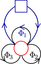
(a) Quiver with one flavor group.

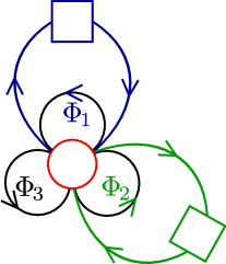
(b) Quiver with two flavor groups.

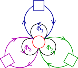
(c) Quiver with three flavor groups.

Figure 3: Quivers for flavored SQED. Circles are gauge groups, squares are flavor groups. Colored arrows indicate bifundamental fields coupled to flavors via a superpotential term.

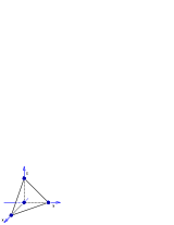
(a) $\mathbb{C}^{4}$

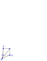
(b) $\mathcal{C}\times\mathbb{C}$

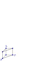
(c) $D_{3}$

Figure 4: Toric diagrams corresponding to some flavors for the $\mathbb{C}^{3}$ quiver.

• In the case $h_{2}=h_{3}=0$, The chiral ring relation is

  $$T\tilde{T}=\Phi_{1}^{h_{1}},$$ (6.5)

  and the geometric branch of the moduli space is $\mathbb{C}^{2}\times\mathbb{C}^{2}/\mathbb{Z}_{h_{1}}$. For $h_{1}=1$ we have $\mathbb{C}^{4}$, see Figure 4(a). This model is related to the dual ABJM model of [11, 16]. We discuss it in a bit more details in Section 6.1.1.

• For $h_{1}=h_{2}=1$, $h_{3}=0$, we have $\mathbb{C}\times\mathcal{C}$ ($\mathcal{C}$ the conifold), see Fig. 4(b). The A-theory for this model is the so-called Phase III of $\mathbb{C}\times\mathcal{C}$ discussed in [16].

• For $h_{1}=2$, $h_{2}=1$, $h_{3}=0$, we have $\mathbb{C}$ times the suspended pinch point (SPP). This was also noticed in [31]. In general, for $h_{1}=a$, $h_{2}=b$, the geometry is $\mathbb{C}\times C(L^{aba})$.

• For $h_{1}=h_{2}=h_{3}=1$, the geometry is $D_{3}$, see Fig. 4(c) . The A-theory for this model is the Phase III of $D_{3}$ discussed in [16].

When some $h_{i}>1$, these geometries have non-isolated singularities. Remark that we have considered the most general toric flavoring of the $\mathbb{C}^{3}$ quiver. The GLSM for the strictly external points is

$$t_{1}$$

(6.6)

This GLSM does not encode various orbifold identifications which might in general arise: for a full description of the geometry one should consider the full GLSM, encoding all the relations in the toric diagram, with $h_{1}+h_{2}+h_{3}+3$ homogeneous coordinates.

6.1.1 Flavoring $\Phi_{1}$: the dual ABJM geometry

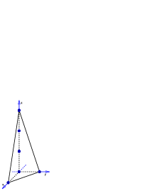
Figure 5: Toric diagrams of $\mathbb{C}^{2}\times\mathbb{C}^{2}/\mathbb{Z}_{h}$, for $h=3$.

Let us discuss a bit more in detail the case $\mathbb{C}^{2}\times\mathbb{C}^{2}/\mathbb{Z}_{h}$. This geometry has the toric diagram shown in Figure 5,

$$a_{0}=(0,0,0),\quad\cdots,\quad a_{h}=(0,0,h),\quad b_{0}=(0,1,0),\quad c_{0}=(1,0,0)$$ (6.7)

There are $h+3$ homogeneous coordinates, and GLSM

$$a_{0}$$

(6.8)

The five affine coordinates are

$$x_{1} =\Phi_{1}=a_{0}a_{1}\dots a_{h-1}a_{h}\;,\;\;\; x_{2} =T=a_{0}^{h}a_{1}^{h-1}\dots a_{h-2}^{2}a_{h-1}\;,$$ (6.9)

$$x_{3} =\tilde{T}=a_{1}a_{2}^{2}\dots a_{h-1}^{h-1}a_{h}^{h}\;, x_{4} =\Phi_{2}=b_{0}\;, x_{5} =\Phi_{3}=c_{0}\;,$$

and of course they satisfy

$$x_{2}x_{3}=x_{1}^{h}.$$ (6.10)

Also, the $Q_{M}$ charges of $(x_{1},\cdots,x_{5})$ are $(0,1,-1,0,0)$, so that $U(1)_{M}$ has fixed points at $x_{2}=x_{3}=0$. Gauging $U(1)_{M}$, we get the type IIA geometry, which is $\mathbb{C}^{3}$ spanned by $(z_{1},z_{2},z_{3})=(x_{1},x_{4},x_{5})$ since the gauge invariant coordinate $x_{2}x_{3}$ can be eliminated by (6.10). The locus of fixed points of $U(1)_{M}$ in the CY₄ descends to the divisor $x_{1}=0$ in $\mathbb{C}^{3}$, where we must have a stack of $h$ D6-branes. This was the argument of section 2, which motivates the field theory we presented.

Note that the same geometry is obtained as the moduli space of the so-called dual ABJM model of [11], at CS level $h$. This model was also studied in [16, 68, 69], and some puzzles were found. At $h=1$, the dual ABJM model corresponds to the A-theory for our flavored theory with a single flavor. For $h$ flavors, our A-theory is a tiling with an $(h+1)$-ple bond. It would be interesting to compare in more details our proposal to the one of [11].

For some specific values of the superpotential couplings, the supersymmetry of our flavored quiver gets enhanced to $\mathcal{N}=4$, since the geometry $\mathbb{C}^{2}\times\mathbb{C}^{2}/\mathbb{Z}_{h}$ is hyper-Kähler. Indeed, our setup is a $\mathcal{N}=2$ version of the setup considered in [64].

6.2 Flavoring the conifold quiver

Consider the quiver of the ABJM theory, equal to the Klebanov-Witten (KW) quiver for D-branes on the conifold $\mathcal{C}$. It has two nodes, four bifundamental fields, $A_{1}$, $A_{2}$, $B_{1}$, $B_{2}$, and superpotential $W=A_{1}B_{1}A_{2}B_{2}-A_{1}B_{2}A_{2}B_{1}$. There are four points in the toric diagram of $\mathbb{C}^{4}/\mathbb{Z}_{k}$, corresponding to the four perfect matchings in the brane tiling of the conifold theory and to the bifundamental fields: because the F-term relations are trivial in the Abelian theory, we can write (with abuse of notation)

$$a_{k} =A_{1}=(0,0,k)\;,\qquad\qquad b_{0} =B_{1}=(0,1,0)\;,$$ (6.11)

$$c_{0} =A_{2}=(1,1,0)\;, d_{0} =B_{2}=(1,0,0)\;.$$

We then consider the toric diagram obtained by adding four columns of points of heights $h_{a}$, $h_{b}$, $h_{c}$, $h_{d}$ above the four base points (any other choice of adding the points above or below, is $SL(4,\mathbb{Z})$ equivalent to this up to a change in $k$):

$$a_{k+i}=(0,0,k+i)\;,\qquad b_{j}=(0,1,j)\;,\qquad c_{l}=(1,1,l)\;,\qquad d_{m}=(1,0,m)\;,$$ (6.12)

where $i=0,\dots,h_{a}$, $j=0,\dots,h_{b}$, $l=0,\dots,h_{c}$, $m=0,\dots,h_{d}$. See Figure 6(b).

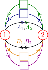
(a) The quiver.

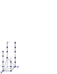
(b) Toric diagram, for $k=2$.

Figure 6: Quiver for a generic flavoring of ABJM, and the corresponding toric diagram, with four columns of heights $h_{a}$, $\cdots$, $h_{d}$.

This toric geometry corresponds to a generic flavoring of the ABJM theory at level $k$, with flavor group $G_{F}=U(h_{a})\times U(h_{b})\times U(h_{c})\times U(h_{d})/U(1)$. The quiver is shown in Figure 6(a), and the superpotential is

$$\begin{split}W&=A_{1}B_{1}A_{2}B_{2}-A_{1}B_{2}A_{2}B_{1}+\\ &+\sum_{i=1}^{h_{a}}p_{1,i}A_{1}q_{1,i}+\sum_{j=1}^{h_{b}}p_{2,j}B_{1}q_{2,j}+\sum_{l=1}^{h_{c}}p_{3,l}A_{2}q_{3,l}+\sum_{r=1}^{h_{d}}p_{4,r}B_{2}q_{4,r}\;.\end{split}$$ (6.13)

Before studying several interesting cases, let us discuss the general solution for the geometric moduli space in this family of models. We have the quantum relation (3.15),

$$T\tilde{T}=A_{1}^{h_{a}}B_{1}^{h_{b}}A_{2}^{h_{c}}B_{2}^{h_{d}}\;,$$ (6.14)

and the CS levels are $(k+f,-k-f)$, with $f=\frac{1}{2}(h_{a}-h_{b}+h_{c}-h_{d})$. The gauge charges of bifundamental fields and monopole operators are (schematically)

$$A_{i}$$

(6.15)

The relation (6.14) can be solved by the perfect matching variables, as

$$A_{1}=\prod_{i=0}^{h_{a}}a_{k+i}\;,\qquad B_{1}=\prod_{j=0}^{h_{b}}b_{j}\;,\qquad A_{2}=\prod_{l=0}^{h_{c}}c_{l}\;,\qquad B_{2}=\prod_{m=0}^{h_{d}}d_{m}$$ (6.16)

and

$$\begin{split}T&=\Big{(}\prod_{i=0}^{h_{a}}a_{k+i}^{h_{a}-i}\Big{)}\Big{(}\prod_{j=0}^{h_{b}}b_{j}^{h_{b}-j}\Big{)}\Big{(}\prod_{l=0}^{h_{c}}c_{l}^{h_{c}-l}\Big{)}\Big{(}\prod_{m=0}^{h_{d}}d_{m}^{h_{d}-m}\Big{)}\\ \tilde{T}&=\Big{(}\prod_{i=0}^{h_{a}}a_{k+i}^{i}\Big{)}\Big{(}\prod_{j=0}^{h_{b}}b_{j}^{j}\Big{)}\Big{(}\prod_{l=0}^{h_{c}}c_{l}^{l}\Big{)}\Big{(}\prod_{m=0}^{h_{d}}d_{m}^{m}\Big{)}\;,\end{split}$$ (6.17)

Notice that each perfect matching variable (6.11) of the ABJM theory is replaced by the product of all GLSM fields associated to the relevant column of points in the toric diagram. Monopole operators are instead products of fields along the four columns, with increasing or decreasing powers as we move vertically. This is to be compared to (B.2). It is easy to show that the $U(1)$ ambiguities of this parametrization reproduce the GLSM associated to the toric diagram (6.12).

6.2.1 Flavoring the field $A_{1}$: the $\mathcal{C}\times\mathbb{C}$ geometry

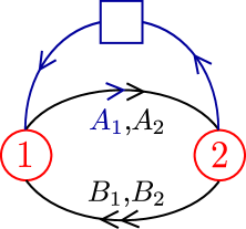
(a) The quiver.

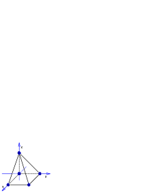
(b) $\mathcal{C}\times\mathbb{C}$

Figure 7: ABJM quiver with one chiral flavor, and its dual geometry.

Let us add a $U(1)$ flavor group to the 3d KW theory ($k=0$), coupled to the bifundamental field $A_{1}$ as in Figure 7(a). The superpotential is $W=A_{1}B_{1}A_{2}B_{2}-A_{1}B_{2}A_{2}B_{1}+pA_{1}q$, and the CS levels are $(\frac{1}{2},-\frac{1}{2})$. The charges of the fields under the gauge and flavor groups are

$$A_{i}$$

1

0

(6.18)

There are seven gauge invariant operators, namely $A_{i}B_{j}$, $TB_{i}$ and $\tilde{T}$. Using the quantum relation $T\tilde{T}=A_{1}$, we can however express $A_{1}B_{i}$ as $\tilde{T}TB_{i}$, so that we actually have only 5 generators of the chiral ring,

$$x_{1}=TB_{1}\;,\quad x_{2}=A_{2}B_{2}\;,\quad x_{3}=TB_{2}\;,\quad x_{4}=A_{2}B_{1}\;,\quad x_{5}=\tilde{T}\;,$$ (6.19)

subject to the relation

$$x_{1}x_{2}-x_{3}x_{4}=0\,.$$ (6.20)

Hence, the moduli space is $\mathcal{C}\times\mathbb{C}$. Indeed, the quantum relation can be solved by $T=a_{0}$, $\tilde{T}=a_{1}$ and $A_{1}=a_{0}a_{1}$. The GLSM is

$$a_{0}$$

(6.21)

where we also specified the $U(1)_{M}$ charges. The toric diagram is shown in Figure 7(b). The locus of fixed points of the $U(1)_{M}$ action descends to the toric divisor $\{a_{0}=0\}$ in the conifold, where the D6-brane sits.

6.2.2 Flavoring the field $A_{1}$: the $C(Y^{2,1}(\mathbb{C}\mathbb{P}^{2}))$ geometry

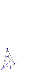
(a) $C(Y^{2,1}(\mathbb{C}\mathbb{P}^{2}))$

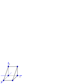
(b) $D_{3}$.

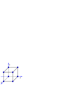
(c) The cubic conifold.

Figure 8: Toric diagrams corresponding to some flavors for the ABJM quiver.

Let us then couple a $U(1)$ flavor group to $A_{1}$ in the ABJM theory at level $k=1$. Now the CS levels are $(\frac{3}{2},-\frac{3}{2})$ and the fields have gauge charges

$$A_{i}$$

2

(6.22)

The quantum relation is solved by $T=a_{1}$, $\tilde{T}=a_{2}$, $A_{1}=a_{1}a_{2}$. The GLSM is

$$a_{1}$$

(6.23)

The corresponding toric diagram is shown in Fig. 8(a), and it corresponds to the cone over $Y^{2,1}(\mathbb{C}\mathbb{P}^{2})$ [70]. This geometry and a related theory (actually the A-theory for our flavored theory) was discussed in [71]. There are nine gauge invariant operators for this quiver, matching the nine affine coordinates of the $C(Y^{2,1}(\mathbb{C}\mathbb{P}^{2}))$ singularity:

$$\begin{array}[]{ccc}\qquad x_{1}=TB_{1}B_{1}=a_{1}b_{0}^{2},&\qquad x_{2}=TB_{2}B_{2}=a_{1}d_{0}^{2},&\qquad x_{3}=\tilde{T}A_{1}=a_{1}a_{2}^{2},\\ \qquad x_{4}=TB_{1}B_{2}=a_{1}b_{0}d_{0},&\qquad x_{5}=A_{1}B_{1}=a_{1}b_{0}a_{2},&\qquad x_{6}=A_{1}B_{2}=a_{1}d_{0}a_{2},\\ \qquad x_{7}=A_{2}B_{1}=b_{0}c_{0},&\qquad x_{8}=A_{2}B_{2}=c_{0}d_{0},&\qquad x_{9}=\tilde{T}A_{2}=c_{0}a_{2}\end{array}$$

The chiral ring relations are:

$$\begin{array}[]{cccc}x_{1}x_{8}=x_{4}x_{7}\;,&x_{2}x_{9}=x_{6}x_{8}\;,&\qquad x_{3}x_{7}=x_{5}x_{9}\;,&\qquad x_{4}x_{9}=x_{5}x_{8}\;,\\ x_{1}x_{9}=x_{5}x_{7}\;,&x_{2}x_{7}=x_{4}x_{8}\;,&\qquad x_{3}x_{8}=x_{6}x_{9}\;,&\qquad x_{4}x_{9}=x_{6}x_{7}\;,\\ x_{1}x_{2}=x_{4}^{2}\;,&x_{1}x_{3}=x_{5}^{2}\;,&\qquad x_{2}x_{3}=x_{6}^{2}\;,\\ x_{1}x_{6}=x_{4}x_{5}\;,&x_{2}x_{5}=x_{4}x_{6}\;,&\qquad x_{3}x_{4}=x_{5}x_{6}\;.\end{array}$$ (6.24)

6.2.3 Flavoring the fields $A_{1}$ and $A_{2}$: the $C(Q^{1,1,1})$ geometry

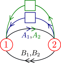
(a) ABJM quiver with two chiral flavor groups.

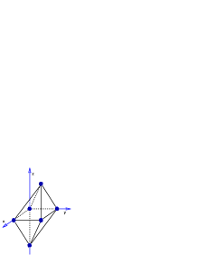
(b) $C(Q^{1,1,1})$.

Figure 9: ABJM quiver with two chiral flavor groups, and a dual geometry.

Consider the conifold quiver with two $U(1)$ flavor groups coupled to $A_{1}$ and $A_{2}$ respectively, as in Fig. 9(a). The superpotential is

$$W=A_{1}B_{1}A_{2}B_{2}-A_{1}B_{2}A_{2}B_{1}+p_{1}A_{1}q_{1}+p_{2}A_{2}q_{2}\;,$$ (6.25)

and we choose vanishing CS levels. In the toric diagram, this corresponds to adding one point below $a_{0}$ and one point above $c_{0}$, see Fig. 9(b). The gauge charges of the fields and monopole operators are

$$A_{i}$$

(6.26)

The monopole operators satisfy the relation

$$T\tilde{T}=A_{1}A_{2}\;.$$ (6.27)

We can solve it by introducing two new perfect matching variables $a_{-1}$ and $c_{1}$:

$$A_{1}=a_{-1}a_{0}, \qquad B_{1}=b_{0}, \qquad T=a_{-1}c_{0},$$ (6.28)

$$A_{2}=c_{0}c_{1}, \qquad B_{2}=d_{0}, \qquad\tilde{T}=a_{0}c_{1}.$$

The associated GLSM is a minimal presentation of the one for the real cone over $Q^{1,1,1}$:

$$a_{0}$$

(6.29)

The gauge invariant operators generating the chiral ring are:

$$\begin{array}[]{ccc}\qquad x_{1}=A_{1}B_{1}=a_{-1}a_{0}b_{0},&\qquad x_{2}=A_{2}B_{2}=c_{0}c_{1}d_{0},&\qquad x_{3}=A_{2}B_{1}=b_{0}c_{0}c_{1},\\ \qquad x_{4}=A_{1}B_{2}=a_{-1}a_{0}d_{0},&\qquad x_{5}=\tilde{T}B_{1}=a_{0}b_{0}c_{1},&\qquad x_{6}=\tilde{T}B_{2}=a_{0}c_{1}d_{0},\\ \qquad x_{7}=TB_{1}=a_{-1}b_{0}c_{0},&\qquad x_{8}=TB_{2}=a_{-1}c_{0}d_{0}.&\end{array}$$

They of course correspond to the affine coordinates on $C(Q^{1,1,1})$, whose algebra is

$$\begin{array}[]{ccc}\qquad x_{1}x_{2}-x_{3}x_{4}=0\;,&\qquad x_{1}x_{2}-x_{5}x_{8}=0\;,&\qquad x_{1}x_{2}-x_{6}x_{7}=0\;,\\ \qquad x_{1}x_{3}-x_{5}x_{7}=0\;,&\qquad x_{1}x_{6}-x_{4}x_{5}=0\;,&\qquad x_{1}x_{8}-x_{4}x_{7}=0\;,\\ \qquad x_{2}x_{4}-x_{6}x_{8}=0\;,&\qquad x_{2}x_{5}-x_{3}x_{6}=0\;,&\qquad x_{2}x_{7}-x_{3}x_{8}=0\;.\end{array}$$ (6.30)

Remark that the affine coordinates have $U(1)_{M}$ charges

$$x_{1}$$

(6.31)

so the $U(1)_{M}$ fixed point locus is at $x_{5}=x_{6}=x_{7}=x_{8}=0$, $x_{1}x_{2}=x_{3}x_{4}=x_{1}x_{3}=x_{2}x_{4}=0$. This locus of fixed points has two branches:

$$1) x_{1}=x_{4}=0\,,\quad x_{5}=x_{6}=x_{7}=x_{8}=0\,,\quad\forall x_{2},\,x_{3} \Longleftrightarrow\quad a_{0}=a_{-1}=0$$ (6.32)

$$2) x_{2}=x_{3}=0\,,\quad x_{5}=x_{6}=x_{7}=x_{8}=0\,,\quad\forall x_{1},\,x_{4} \Longleftrightarrow\quad c_{0}=c_{1}=0\;.$$

It is easy to see that they descend to the toric divisors $\{a_{0}=0\}$ and $\{c_{0}=0\}$ in the conifold $\mathcal{C}$. The D6-branes wrapping these divisors provide us with the chiral flavors in the quiver field theory.

Another quiver for the low energy field theory on M2-branes on $C(Q^{1,1,1})$ was proposed in [12], and further studied in [15]. The quiver of [12], which has two double-bonds, is precisely the A-theory of our chirally flavored conifold theory.

6.2.4 Flavoring the fields $A_{1}$ and $B_{1}$: the $D_{3}$ geometry

Let us now couple a $U(1)$ flavor group to $A_{1}$ and a $U(1)$ flavor group to $B_{1}$, with $\delta W=p_{1}A_{1}q_{1}+\tilde{p}_{1}B_{1}\tilde{q}_{1}$ and vanishing CS levels. In this case there is no induced gauge charge for the monopole operators, because there are as many incoming as outgoing arrows in each gauge group. We have the quantum relation $T\tilde{T}=A_{1}B_{1}$, which is solved by $A_{1}=a_{0}a_{1}$, $B_{1}=b_{0}b_{1}$, $T=a_{0}b_{0}$ and $\tilde{T}=a_{1}b_{1}$. The associated GLSM is

$$a_{0}$$

(6.33)

The toric diagram, shown in Fig. 8(b), is the one of the $D_{3}$ geometry. The generators of the chiral ring are

$$x_{1}=\tilde{T}\;,\quad x_{2}=A_{2}B_{2}\;,\quad x_{3}=T\;,\quad x_{4}=A_{1}B_{2}\;,\quad x_{5}=A_{2}B_{1}\;.$$ (6.34)

As expected, they satisfy the defining equation of the $D_{3}$ singularity:

$$x_{1}x_{2}x_{3}-x_{4}x_{5}=0\;.$$ (6.35)

The locus of fixed points of $U(1)_{M}$ has two branches which descend to the two divisors $\{a_{0}=0\}$ and $\{b_{0}=0\}$ in the conifold.

6.2.5 Flavoring $A_{1}$, $A_{2}$, $B_{1}$, $B_{2}$: the cubic conifold

Consider coupling a $U(1)$ flavor group to each bifundamental field, with vanishing CS levels. The quantum relation is

$$T\tilde{T}=A_{1}B_{1}A_{2}B_{2}\;.$$ (6.36)

One can check that the moduli space is described by the following GLSM:

$$a_{0}$$

(6.37)

The toric diagram is shown in Fig. 8(c), and we will call this geometry the cubic conifold. The gauge invariant operators are

$$\begin{array}[]{ccc}\qquad x_{1}=a_{0}b_{0}c_{0}d_{0}=T,&\qquad x_{2}=a_{1}b_{1}c_{1}d_{1}=\tilde{T},&\qquad x_{3}=a_{0}b_{0}a_{1}b_{1}=A_{1}B_{1},\\ \qquad x_{4}=c_{0}d_{0}c_{1}d_{1}=A_{2}B_{2},&\qquad x_{5}=a_{0}d_{0}a_{1}d_{1}=A_{1}B_{2},&\qquad x_{6}=b_{0}c_{0}b_{1}c_{1}=A_{2}B_{1},\end{array}$$

satisfying the equations

$$x_{1}x_{2}-x_{3}x_{4}=0\;,\qquad\qquad x_{1}x_{2}-x_{5}x_{6}=0\;.$$ (6.38)

This is a complete intersection. The $U(1)_{M}$ charges of $(x_{1},\cdots,x_{6})$ are $(1,-1,0,0,0,0)$. The locus of fixed point is at $x_{1}=x_{2}=0$, $x_{3}x_{4}=x_{5}x_{6}=0$, which has four branches and descend to the four toric divisors of the conifold.

6.3 Flavoring the modified $\mathbb{C}\times\mathbb{C}^{2}/\mathbb{Z}_{2}$ theory

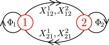
(a) The $A_{1}$ quiver.

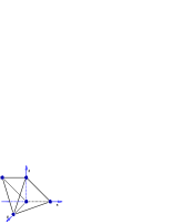
(b) $\mathbb{C}\times\mathcal{C}$.

Figure 10: Quiver of the modified $\mathbb{C}\times\mathbb{C}^{2}/\mathbb{Z}_{2}$ model (CS levels $(1,-1)$), and moduli space.

In this section we add flavors to the so-called modified $\mathbb{C}\times\mathbb{C}^{2}/\mathbb{Z}_{2}$ theory of [8]. The quiver of the unflavored theory, Fig. 10(a), is the one for D-branes at a $\mathbb{C}\times\mathbb{C}^{2}/\mathbb{Z}_{2}$ singularity; we choose the height numbers $n_{ij}$ equal to $1$ for the bifundamental $X_{12}^{1}$ and $0$ otherwise, so that the two gauge groups have CS levels $(1,-1)$. The superpotential is

$$W=\Phi_{1}(X_{12}^{1}X_{21}^{2}-X_{12}^{2}X_{21}^{1})-\Phi_{2}(X_{21}^{2}X_{12}^{1}-X_{21}^{1}X_{12}^{2})\;.$$ (6.39)

From the permanent of the Kasteleyn matrix,

$$\mathrm{Perm}\,K=X_{21}^{1}X_{21}^{2}+X_{12}^{2}X_{21}^{2}\,x+X_{21}^{1}X_{12}^{1}\,x^{-1}z+X_{12}^{1}X_{12}^{2}\,z+\Phi_{1}\Phi_{2}\,y\;,$$ (6.40)

we see that the perfect matchings are

$$\begin{array}[]{cccc}\quad a_{0}&=\{X_{21}^{1},X_{21}^{2}\}=(0,0,0),&\qquad d_{1}&=\{X_{12}^{1},X_{12}^{2}\}=(0,0,1),\\ \quad b_{0}&=\{X_{12}^{2},X_{21}^{2}\}=(1,0,0),&\qquad e_{0}&=\{\Phi_{1},\Phi_{2}\}=(0,1,0),\\ \quad c_{1}&=\{X_{21}^{1},X_{12}^{1}\}=(-1,0,1).&&\end{array}$$ (6.41)

The 3d toric diagram, Fig. 10(b), is the one of $\mathbb{C}\times\mathcal{C}$. The F-term equations imply $X_{12}^{1}X_{21}^{2}=X_{12}^{2}X_{21}^{1}$ and $\Phi_{1}=\Phi_{2}$ along the mesonic branch. They are solved by

$$X_{12}^{1}=c_{1}\,d_{1}\;,\quad X_{12}^{2}=b_{0}\,d_{1}\;,\quad X_{21}^{1}=a_{0}\,c_{1}\;,\quad X_{21}^{2}=a_{0}\,b_{0}\;,\quad\Phi_{1}=\Phi_{2}=e_{0}\;.$$

The face in the 3d toric diagram whose vertices are $\{a_{0},c_{1},d_{1},b_{0}\}$ is vertical, therefore additional objects may appear in the type IIA background. Nevertheless, encouraged by the results of [8] where the geometric moduli space was successfully matched with $\mathbb{C}\times\mathcal{C}$, we will trust the duality and add flavors to this model.

We will study three illustrative examples where two flavor pairs are added to this theory.

6.3.1 $U(2)$ flavor group coupled to $X_{12}^{1}$: levels $(0,0)$

(a) CS levels $(0,0)$.

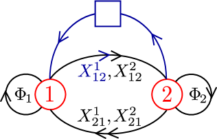
(b) One flavored bifundamental.

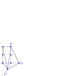
(c) CS levels $(1,-1)$.

Figure 11: The $\mathbb{C}\times\mathbb{C}^{2}/\mathbb{Z}_{2}$ quiver with a $U(2)$ flavor group coupled to $X_{12}^{1}$. Those two toric quivers are obtained by fixing the CS levels as indicated.

We study two cases where we couple a $U(2)$ flavor group to $X_{12}^{1}$, as in Fig. 11(b). Consider first the case where the CS levels vanish. The bifundamental fields and monopole operators of the quiver theory have gauge charges

$$X_{12}$$

(6.42)

The gauge invariant operators in the geometric branch are $\Phi$, $X_{12}X_{21}$, $TX_{21}$, $\tilde{T}X_{21}$.

In the A-theory, this flavoring corresponds to replacing the edge $X_{12}^{1}$ with $n_{X_{12}^{1}}=1$ in the original brane tiling with a triple-bond with $n=-1,0,1$. It amounts to considering a 3d toric diagram with the points $\{a_{0},b_{0},c_{-1},c_{0},c_{1},d_{-1},d_{0},d_{1},e_{0}\}$ as in Fig. 11(a). We solve for the F-term relation and the quantum relation $T\tilde{T}=X^{1}_{12}$ by

$$X_{12}^{1} =c_{-1}\,c_{0}\,c_{1}\,d_{-1}\,d_{0}\,d_{1}\;,\qquad X_{12}^{2} =b_{0}\,d_{-1}\,d_{0}\,d_{1}\;,\qquad$$ (6.43)

$$X_{21}^{1} =a_{0}\,c_{-1}\,c_{0}\,c_{1}\;, X_{21}^{2} =a_{0}\,b_{0}\;, \Phi_{1} =\Phi_{2}=e_{0}\;,$$

$$\tilde{T} =c_{0}\,c_{1}^{2}\,d_{0}\,d_{1}^{2}\;, T =c_{-1}^{2}\,c_{0}\,d_{-1}^{2}\,d_{0}\;.$$

The charges of the homogeneous coordinates of the four-fold and of the quiver theory fields under the associated $U(1)^{5}$ GLSM are

$$a_{0}$$

matching the gauge charges (6.42). The affine coordinates of the fourfold match the gauge invariant operators of the flavored quiver theory:

$$\begin{split}&x_{1}=e_{0}=\Phi_{1}=\Phi_{2}\;,\qquad\qquad\qquad\qquad\quad x_{2}=a_{0}\,b_{0}^{2}\,d_{-1}\,d_{0}\,d_{1}=X_{12}^{2}X_{21}^{2}\;,\\ &x_{3}=a_{0}\,b_{0}\,c_{0}\,c_{1}^{2}\,d_{0}\,d_{1}^{2}=\tilde{T}X_{21}^{2}\;,\qquad\qquad\quad x_{4}=a_{0}\,c_{-1}\,c_{0}^{2}\,c_{1}^{3}\,d_{0}\,d_{1}^{2}=\tilde{T}X_{21}^{1}\;,\\ &x_{5}=a_{0}\,b_{0}\,c_{-1}\,c_{0}\,c_{1}\,d_{-1}\,d_{0}\,d_{1}=X_{12}^{1}X_{21}^{2}=X_{12}^{2}X_{21}^{1}\;,\\ &x_{6}=a_{0}\,c_{-1}^{2}\,c_{0}^{2}\,c_{1}^{2}\,d_{-1}\,d_{0}\,d_{1}=X_{12}^{1}X_{21}^{1}\;,\\ &x_{7}=a_{0}\,b_{0}\,c_{-1}^{2}\,c_{0}\,d_{-1}^{2}\,d_{0}=TX_{21}^{2}\;,\qquad\quad\quad x_{8}=a_{0}\,c_{-1}^{3}\,c_{0}^{2}\,c_{1}\,d_{-1}^{2}\,d_{0}=TX_{21}^{1}\;.\end{split}$$ (6.44)

6.3.2 $U(2)$ flavor group coupled to $X_{12}^{1}$: levels $(1,-1)$

Consider now the case of CS levels $(1,-1)$. The gauge charges are:

$$X_{12}$$

2

2

(6.45)

The gauge invariant operators are $\Phi$, $X_{12}X_{21}$, $T(X_{21})^{2}$, $\tilde{T}$.

In the A-theory, this flavoring corresponds to replacing the edge $X_{12}^{1}$ with $n_{X_{12}^{1}}=1$ in the original brane tiling by a triple-bond with $n=0,1,2$. The GLSM field appearing in the 3d toric diagram, Fig. 11(c), are $\{a_{0},b_{0},c_{0},c_{1},c_{2},d_{0},d_{1},d_{2},e_{0}\}$. We solve for the geometric moduli space by setting

$$X_{12}^{1} =c_{0}\,c_{1}\,c_{2}\,d_{0}\,d_{1}\,d_{2}\;,\qquad X_{12}^{2} =b_{0}\,d_{0}\,d_{1}\,d_{2}\;,\qquad$$ (6.46)

$$X_{21}^{1} =a_{0}\,c_{0}\,c_{1}\,c_{2}\;, X_{21}^{2} =a_{0}\,b_{0}\;, \Phi_{1} =\Phi_{2}=e_{0}\;,$$

$$\tilde{T} =c_{1}\,c_{2}^{2}\,d_{1}\,d_{2}^{2}\;, T =c_{0}^{2}\,c_{1}\,d_{0}^{2}\,d_{1}\;.$$

The charges of the homogeneous coordinates of the fourfold and of the quiver theory fields under the $U(1)^{5}$ GLSM are

$$a_{0}$$

matching the gauge charges (6.45). The affine coordinates of the four-fold match the holomorphic gauge invariants of the flavored quiver theory:

$$\begin{split}&x_{1}=a_{0}\,b_{0}\,c_{0}\,c_{1}\,c_{2}\,d_{0}\,d_{1}\,d_{2}=X_{12}^{1}X_{21}^{2}=X_{12}^{2}X_{21}^{1}\;,\quad x_{2}=e_{0}=\Phi_{1}=\Phi_{2}\;,\\ &x_{3}=a_{0}^{2}\,b_{0}^{2}\,c_{0}^{2}\,c_{1}\,d_{0}^{2}\,d_{1}=T(X_{21}^{2})^{2}\;,\qquad\qquad\quad\quad\;\;\;\;\,x_{4}=a_{0}\,c_{0}^{2}\,c_{1}^{2}\,c_{2}^{2}\,d_{0}\,d_{1}\,d_{2}=X_{12}^{1}X_{21}^{1}\;,\\ &x_{5}=a_{0}^{2}\,b_{0}\,c_{0}^{3}\,c_{1}^{2}\,c_{2}\,d_{0}^{2}\,d_{1}=TX_{21}^{1}X_{21}^{2}\;,\qquad\qquad\quad\;\;\;x_{6}=a_{0}\,b_{0}^{2}\,d_{0}\,d_{1}\,d_{2}=X_{12}^{2}X_{21}^{2}\;,\\ &x_{7}=a_{0}^{2}\,c_{0}^{4}\,c_{1}^{3}\,c_{2}^{2}\,d_{0}^{2}\,d_{1}=T(X_{21}^{1})^{2}\;,\qquad\qquad\qquad\quad\;x_{8}=c_{1}\,c_{2}^{2}\,d_{1}\,d_{2}^{2}=\tilde{T}\;.\end{split}$$

6.3.3 $U(1)^{2}$ flavor groups coupled to $X_{12}^{1}$ and $X_{21}^{1}$: levels $(1,-1)$

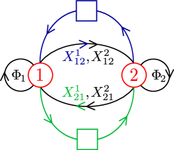
(a) The quiver.

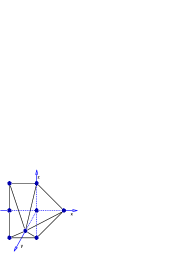
(b) Toric diagram when the CS levels are $(1,-1)$.

Figure 12: Modified $\mathbb{C}\times\mathbb{C}^{2}/\mathbb{Z}_{2}$ model with two flavored bifundamentals, and dual geometry.

Let us study a case where we couple a $U(1)$ flavor group to $X_{12}^{1}$ and a $U(1)$ flavor group to $X_{21}^{1}$, as in Fig. 12(a). The quantum relation reads ${T}\tilde{T}=X_{12}^{1}X_{12}^{2}$. We consider the case with CS levels $(1,-1)$: bifundamentals and monopole operators charges are

$$X_{12}$$

(6.47)

The gauge invariant operators are $\Phi$, $X_{12}X_{21}$, $TX_{21}$, $\tilde{T}X_{12}$.

In the A-theory, this flavoring corresponds to replacing the edge $X_{12}^{1}$ with $n_{X_{12}^{1}}=1$ in the brane tiling by a double-bond with $n=0,1$, and the edge $X_{21}^{1}$ with $n_{X_{21}^{1}}=0$ by another double-bond, with $n=-1,0$. All the other $n_{ij}$ vanish. This gives a 3d toric diagram with points $\{a_{-1},a_{0},b_{0},c_{-1},c_{0},c_{0}^{\prime},c_{1},d_{0},d_{1},e_{0}\}$, Fig. 12(b). This is not a minimal presentation of the toric diagram. In particular, unlike for the other multiplicities, the distinction between $c_{0}$ and $c_{0}^{\prime}$ is not needed to express the bifundamentals and monopole operators in terms of GLSM fields solving the F-term equations. It is possible to replace the two of them by a single field $\tilde{c}_{0}$ (setting $c_{0}\,c_{0}^{\prime}=\tilde{c}_{0}$ in the formulæ below), getting rid of a $U(1)$ in the GLSM. We will do that in the following. Keeping instead all the perfect matching fields of the A-theory may be useful in the study of partial resolutions dual to real mass terms.

We solve for the geometric moduli space by setting

$$X_{12}^{1} =c_{-1}\,\tilde{c}_{0}\,c_{1}\,d_{0}\,d_{1}\;,\qquad X_{12}^{2} =b_{0}\,d_{0}\,d_{1}\;,\qquad$$ (6.48)

$$X_{21}^{1} =a_{-1}\,a_{0}\,c_{-1}\,\tilde{c}_{0}\,c_{1}\;, X_{21}^{2} =a_{-1}\,a_{0}\,b_{0}\;, \Phi_{1} =\Phi_{2}=e_{0}\;,$$

$$\tilde{T} =a_{0}\,\tilde{c}_{0}\,c_{1}^{2}\,d_{1}\;, T =a_{-1}\,c_{-1}^{2}\,\tilde{c}_{0}\,d_{0}\;.\qquad$$

The charges of the homogeneous coordinates of the four-fold and of the quiver theory fields under the resulting $U(1)^{5}$ GLSM are

$$a_{0}$$

matching the gauge charges (6.47). The affine coordinates of the four-fold match the holomorphic gauge invariants of the flavored quiver theory:

$$\begin{split}&x_{1}=e_{0}=\Phi_{1}=\Phi_{2}\;,\qquad\qquad\qquad\qquad\qquad\;x_{2}=a_{-1}\,a_{0}\,b_{0}^{2}\,d_{0}\,d_{1}=X_{12}^{2}X_{21}^{2}\;,\\ &x_{3}=a_{-1}^{2}\,a_{0}\,c_{-1}^{3}\,c_{0}^{2}\,c_{0}^{\prime 2}\,c_{1}\,d_{0}=TX_{21}^{1}\;,\qquad\qquad x_{4}=a_{0}\,c_{-1}\,c_{0}^{2}\,c_{0}^{\prime 2}\,c_{1}^{3}\,d_{0}\,d_{1}^{2}=\tilde{T}X_{12}^{1}\;,\\ &x_{5}=a_{-1}^{2}\,a_{0}\,b_{0}\,c_{-1}^{2}\,c_{0}\,c_{0}^{\prime}\,d_{0}=TX_{21}^{2}\;,\qquad\qquad\,x_{6}=a_{0}\,b_{0}\,c_{0}\,c_{0}^{\prime}\,c_{1}^{2}\,d_{0}\,d_{1}^{2}=\tilde{T}X_{12}^{2}\;,\\ &x_{7}=a_{-1}\,a_{0}\,c_{-1}^{2}\,c_{0}^{2}\,c_{0}^{\prime 2}\,c_{1}^{2}\,d_{0}\,d_{1}=X_{12}^{1}X_{21}^{1}=\tilde{T}T\;,\\ &x_{8}=a_{-1}\,a_{0}\,b_{0}\,c_{-1}\,c_{0}\,c_{0}^{\prime}\,c_{1}\,d_{0}\,d_{1}=X_{12}^{1}X_{21}^{2}=X_{12}^{2}X_{21}^{1}\;.\end{split}$$ (6.49)

The toric diagram of the CY₄ is the same as in the double-flavored $X_{12}^{1}$ model with CS levels $(0,0)$ studied in subsection 6.3.1: thus the geometric branches of the moduli spaces of these two theories are the same, although the manifest flavor symmetries of the quivers are different. Presumably, the M-theory backgrounds will differ in monodromies of the 3-form potential $C_{3}$.

The three double flavored models analyzed here for the modified $\mathbb{C}\times\mathbb{C}^{2}/\mathbb{Z}_{2}$ model lead to D6-branes along the same toric divisor inside the CY₃. However there are different gauge connections on the flavor branes, everywhere flat but at the tip, and gauge fluxes on the 2-cycles at the singularity. In spite of the D6-branes being identically embedded at the level of the complex structure, the type IIA/M-theory backgrounds differ, because the different gauge fluxes at the singularity generate RR fluxes that backreact onto the metric.

6.4 Flavoring the $dP_{0}$ quiver

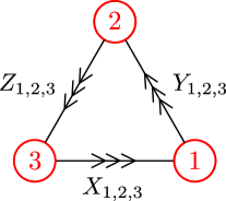
(a) The quiver.

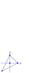
(b) The 2d toric diagram.

Figure 13: The $dP_{0}$ quiver and the 2d toric diagram.

The $dP_{0}$ quiver, Fig. 13(a), is the quiver for D-branes at a $\mathbb{C}^{3}/\mathbb{Z}_{3}$ singularity. It has three nodes and nine bifundamental fields, $X_{i}$, $Y_{i}$, $Z_{i}$, $i=1,2,3$. We choose to parametrize the CS levels by $(k_{1},k_{2},k_{3})=(q-p,q,p-2q)$. The charges under the $U(1)^{3}$ gauge group are

$$X_{i}$$

(6.50)

The superpotential is $W=X_{i}Y_{j}Z_{k}\epsilon^{ijk}$, so the indices $ijk$ are fully symmetric in the chiral ring. From the permanent of the Kasteleyn matrix,

$$\mathrm{Perm}\,K=X_{1}Y_{1}Z_{1}xz^{p}+X_{2}Y_{2}Z_{2}x^{-1}y^{-1}+X_{3}Y_{3}Z_{3}y+X_{1}X_{2}X_{3}z^{p-q}+Y_{1}Y_{2}Y_{3}z^{q}+Z_{1}Z_{2}Z_{3},$$

we read off the perfect matchings and the coordinates of the points in the toric diagram:

$$\begin{array}[]{cc}\quad a_{p}=\{X_{1},Y_{1},Z_{1}\}\,=\,(1,0,p)\;,&\quad e_{p-q}=\{X_{1},X_{2},X_{3}\}\,=\,(0,0,p-q)\;,\\ \quad b_{0}=\{X_{2},Y_{2},Z_{2}\}\,=\,(0,1,0)\;,&\quad f_{q}=\{Y_{1},Y_{2},Y_{3}\}\,=\,(0,0,q)\;,\\ \quad c_{0}=\{X_{3},Y_{3},Z_{3}\}\,=\,(-1,-1,0)\;,&\quad g_{0}=\{Z_{1},Z_{2},Z_{3}\}\,=\,(0,0,0)\;.\end{array}$$ (6.51)

The choice of $SL(4,\mathbb{Z})$ frame is such that for $p,q>0$ we have the geometry $Y^{p,q}(\mathbb{C}\mathbb{P}^{2})$ as presented in [70]. In particular, this family includes the geometry $M^{3,2}=Y^{3,2}(\mathbb{C}\mathbb{P}^{2})$. The perfect matching variables allow to solve the F-term relations as

$$\begin{array}[]{ccc}\qquad X_{1}=a_{p}e_{p-q}\;,&\qquad Y_{1}=a_{p}f_{q}\;,&\qquad Z_{1}=a_{p}g_{0}\;,\\ \qquad X_{2}=b_{0}e_{p-q}\;,&\qquad Y_{2}=b_{0}f_{q}\;,&\qquad Z_{2}=b_{0}g_{0}\;,\\ \qquad X_{3}=c_{0}e_{p-q}\;,&\qquad Y_{3}=c_{0}f_{q}\;,&\qquad Z_{3}=c_{0}g_{0}\;,\end{array}$$ (6.52)

and the redundancies in this parametrization correspond to a non-minimal GLSM for the toric geometry. We couple chiral flavors to bifundamental fields in the $dP_{0}$ quiver, and consider a few simple but interesting examples, flavoring the theory with vanishing CS levels $p=q=0$. The 2d diagram is shown in Fig. 13(b).

6.4.1 $U(1)$ flavor group coupled to $X_{1}$

Let us couple one flavor to the field $X_{1}$ in the quiver with vanishing CS levels, which induces CS levels $(-\frac{1}{2},0,\frac{1}{2})$. The quantum relation is $T\tilde{T}=X_{1}$, and the gauge charges of the fields and monopole operators are:

$$X_{i}$$

1

(6.53)

To find the geometric branch of the moduli space, we solve both the F-terms and the quantum relation by adding two new variables $a_{1}$ and $e_{1}$ to the solution (6.52):

$$\begin{array}[]{cccc}\qquad X_{1}=a_{0}a_{1}e_{0}e_{1}\;,&\qquad Y_{1}=a_{0}a_{1}f_{0}\;,&\qquad Z_{1}=a_{0}a_{1}g_{0}\;,&\qquad T=a_{0}e_{0}\;,\\ \qquad X_{2}=b_{0}e_{0}e_{1}\;,&\qquad Y_{2}=b_{0}f_{0}\;,&\qquad Z_{2}=b_{0}g_{0}\;,&\qquad\tilde{T}=a_{1}e_{1}\;,\\ \qquad X_{3}=c_{0}e_{0}e_{1}\;,&\qquad Y_{3}=c_{0}f_{0}\;,&\qquad Z_{3}=c_{0}g_{0}\;.\end{array}$$ (6.54)

The associated GLSM is

$$a_{0}$$

(6.55)

The three first rows correspond to the gauge group $U(1)^{3}$ of the quiver. This GLSM is a non-minimal presentation of the toric geometry of Fig. 14(a), corresponding to adding two points $a_{1}$ and $e_{1}$ as suggested by the A-theory. We have also specified the $Q_{M}$ charges. Gauging $U(1)_{M}$ leads to the CY₃ $\mathbb{C}^{3}/\mathbb{Z}_{3}$, and the locus of fixed points projects to the non-compact divisor $\{a_{0}=0\}$. Let us check that the gauge invariant operators match the affine coordinates of the toric variety. There are 10 operators of the form $XYZ$, 6 of the form $TYZ$, and $\tilde{T}$, but the quantum relation makes $X_{1}YZ=\tilde{T}TYZ$ redundant, so that we are left with 11 generators of the chiral ring. We can check that they match all the gauge invariant functions of the GLSM:

$$\begin{array}[]{ccc}x_{1}=TY_{1}Z_{1}=a_{0}^{3}e_{0}f_{0}g_{0}a_{1}^{2}\;,&\qquad x_{6}=TY_{2}Z_{2}=a_{0}b_{0}^{2}e_{0}f_{0}g_{0}\;,&\quad x_{11}=\tilde{T}=a_{1}e_{1}\;.\\ x_{2}=X_{2}Y_{2}Z_{2}=b_{0}^{3}e_{0}f_{0}g_{0}e_{1}\;,&\qquad x_{7}=X_{2}Y_{2}Z_{3}=b_{0}^{2}c_{0}e_{0}f_{0}g_{0}e_{1}\;,\\ x_{3}=X_{3}Y_{3}Z_{3}=c_{0}^{3}e_{0}f_{0}g_{0}e_{1}\;,&\qquad x_{8}=TY_{3}Z_{3}=a_{0}c_{0}^{2}e_{0}f_{0}g_{0}\;,\\ x_{4}=TY_{1}Z_{2}=a_{0}^{2}b_{0}e_{0}f_{0}g_{0}a_{1}\;,&\qquad x_{9}=X_{2}Y_{3}Z_{3}=b_{0}c_{0}^{2}e_{0}f_{0}g_{0}e_{1}\;,\\ x_{5}=TY_{1}Z_{3}=a_{0}^{2}c_{0}e_{0}f_{0}g_{0}a_{1}\;,&\qquad x_{10}=TY_{2}Z_{3}=a_{0}b_{0}c_{0}e_{0}f_{0}g_{0}\;,\end{array}$$

6.4.2 $U(1)^{2}$ flavor groups coupled to $X_{1}$ and $Y_{1}$

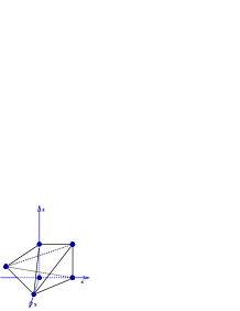
(a)

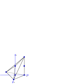
(b)

Figure 14: Toric diagram obtained by flavoring one or two fields in the $dP_{0}$ quiver.

Consider flavoring $X_{1}=ae$ and $Y_{1}=ef$. There are two possible CS levels, but let us consider the case $(0,-\frac{1}{2},\frac{1}{2})$ corresponding to adding four perfect matching variables $a_{1}$, $a_{2}$, $e_{1}$, $f_{1}$. The toric diagram is in Fig. 14(b). The field theory gauge charges are

$$X_{i}$$

0

1 0

(6.56)

The quantum relation is $T\tilde{T}=X_{1}Y_{1}$. There are again 11 gauge invariant operators: $X_{i}Y_{j}Z_{k}$, $TZ_{i}$ and $\tilde{T}$, but the three operators $X_{1}Y_{1}Z_{i}$ are redundant due to the quantum relation. We can solve the moduli space equations by

$$\begin{array}[]{cccc}X_{1}=a_{0}a_{1}a_{2}e_{0}e_{1}\;,&\qquad Y_{1}=a_{0}a_{1}a_{2}f_{0}f_{1}\;,&\qquad Z_{1}=a_{0}a_{1}a_{2}g_{0}\;,&\qquad T=a_{0}^{2}a_{1}e_{0}f_{0}\;,\\ X_{2}=b_{0}e_{0}e_{1}\;,&\qquad Y_{2}=b_{0}f_{0}f_{1}\;,&\qquad Z_{2}=b_{0}g_{0}\;,&\qquad\tilde{T}=a_{1}a_{2}^{2}e_{1}f_{1}\;.\\ X_{3}=c_{0}e_{0}e_{1}\;,&\qquad Y_{3}=c_{0}f_{0}f_{1}\;,&\qquad Z_{3}=c_{0}g_{0}\;,\end{array}$$

and the associated GLSM is

$$a_{0}$$

(6.57)

The map between affine coordinates and gauge invariant operators is

$$\begin{array}[]{cc}\qquad x_{1}=TZ_{1}=a_{0}^{3}a_{1}^{2}a_{2}e_{0}f_{0}g_{0}\;,&\qquad\qquad x_{6}=X_{1}Y_{2}Z_{2}=a_{0}a_{1}a_{2}b_{0}^{2}e_{0}e_{1}f_{0}f_{1}g_{0}\;,\\ \qquad x_{2}=X_{2}Y_{2}Z_{2}=b_{0}^{3}e_{0}e_{1}f_{0}f_{1}g_{0}\;,&\qquad\qquad x_{7}=X_{2}Y_{2}Z_{3}=b_{0}^{2}c_{0}e_{0}e_{1}f_{0}f_{1}g_{0}\;,\\ \qquad x_{3}=X_{3}Y_{3}Z_{3}=c_{0}^{3}e_{0}e_{1}f_{0}f_{1}g_{0}\;,&\qquad\qquad x_{8}=X_{1}Y_{3}Z_{3}=a_{0}a_{1}a_{2}c_{0}^{2}e_{0}e_{1}f_{0}f_{1}g_{0}\;,\\ \qquad x_{4}=TZ_{2}=a_{0}^{2}a_{1}b_{0}e_{0}f_{0}g_{0}\;,&\qquad\qquad x_{9}=X_{2}Y_{3}Z_{3}=b_{0}c_{0}^{2}e_{0}e_{1}f_{0}f_{1}g_{0}\;,\\ \qquad x_{5}=TZ_{3}=a_{0}^{2}a_{1}ce_{0}f_{0}g_{0}\;,&\qquad\qquad x_{10}=X_{1}Y_{2}Z_{3}=a_{0}a_{1}a_{2}b_{0}c_{0}e_{0}e_{1}f_{0}f_{1}g_{0}\;,\\ &\qquad\qquad x_{11}=\tilde{T}=a_{1}a_{2}^{2}e_{1}f_{1}\;.\end{array}$$

6.5 Flavoring the $dP_{1}$ quiver

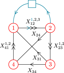
(a) The quiver.

(b) Toric diagram.

Figure 15: The $dP_{1}$ quiver with one flavor. Flavoring $X_{12}^{1}$ has the effect of adding a new point above two external points and one internal point in the toric diagram.

The $dP_{1}$ quiver describes D-branes at the $C(Y^{2,1})$ CY₃ singularity. The quiver has 4 nodes and 10 bifundamental fields, as reviewed in Appendix A. The brane tiling is shown in Fig. 16 and its perfect matchings are given in (A.9). Consider coupling a single flavor to the field $X_{12}^{1}$, as in Figure 15(a). This time the field we flavor corresponds to two external points $b_{0}$ and $c_{0}$, , as well as an internal point $e_{0}$, in the toric diagram of $dP_{1}$. The Chern-Simons levels are $(\frac{1}{2},-\frac{1}{2},0,0)$, which corresponds to adding three points $b_{1}$, $c_{1}$ and $e_{1}$ in the toric diagram, as shown in Figure 15(b).

$$X_{12}^{j}$$

1

(6.58)

The quantum relation is $T\tilde{T}=X_{12}^{1}$. The F-term equations are solved by

$$\begin{array}[]{cccc}X_{12}^{1}=b_{0}b_{1}c_{0}c_{1}e_{0}e_{1}\;,&\qquad X_{41}^{1}=c_{0}c_{1}h_{0}\;,&\qquad X_{23}^{1}=c_{0}c_{1}f_{0}\;,&\qquad X_{34}=b_{0}b_{1}g_{0}\;,\\ X_{12}^{2}=a_{0}b_{0}b_{1}e_{0}e_{1}\;,&\qquad X_{41}^{2}=a_{0}h_{0}\;,&\qquad X_{23}^{2}=a_{0}f_{0}\;,&\qquad T=b_{0}c_{0}e_{0}\;,\\ X_{12}^{3}=d_{0}e_{0}e_{1}\;,&\qquad X_{31}=d_{0}g_{0}h_{0}\;,&\qquad X_{24}=d_{0}f_{0}g_{0}\;,&\qquad\tilde{T}=b_{1}c_{1}e_{1}\;.\end{array}$$

The GLSM is

$$a_{0}$$

(6.59)

The three first lines correspond to the gauge charges under the first three gauge groups. Using the F-term relations together with $T\tilde{T}=X_{12}^{1}$, one can show that there are only 10 independent generators of the chiral ring,

$$\begin{array}[]{cccc}x_{1}=X_{12}^{3}X_{24}X_{41}^{1}\;,&\qquad x_{4}=TX_{24}X_{41}^{2}\;,&\qquad x_{7}=TX_{23}^{1}X_{34}X_{41}^{2}\;,&\quad x_{10}=\tilde{T}\;.\\ x_{2}=X_{12}^{3}X_{24}X_{41}^{2}\;,&\qquad x_{5}=X_{12}^{3}X_{23}^{2}X_{34}X_{41}^{2}\;,&\qquad x_{8}=TX_{23}^{2}X_{34}X_{41}^{2}\;,\\ x_{3}=TX_{24}X_{41}^{1}\;,&\qquad x_{6}=TX_{23}^{1}X_{34}X_{41}^{1}\;,&\qquad x_{9}=X_{12}^{2}X_{23}^{2}X_{34}X_{41}^{2}\;.\end{array}$$

and that they match the 10 affine coordinates of the toric geometry of Figure 15(b).

7 Conclusions

In this paper we studied the chiral ring of CFTs describing the IR fixed point of general 3d $\mathcal{N}=2$ supersymmetric quiver gauge theories with chiral flavors, with or without CS terms, focusing on the toric case. These CFTs are conjectured to be holographically dual to M-theory on $AdS_{4}\times H_{7}$ backgrounds.

We have generalized the stringy derivation of the quiver theories [17] to cases where the M-theory circle degenerates at complex codimension-two loci in the toric $CY_{4}$ cone, leading to flavor D6-branes wrapping toric divisors of the fibered $CY_{3}$ in type IIA string theory. The holomorphic embedding of flavor branes determines the superpotential couplings between the (anti)fundamental flavor superfields and bifundamental matter in the dual theory, whereas the RR $F_{2}$ fluxes contributed by D6-branes shift the CS levels.

Conversely, we have studied the addition of flavors coupled to bifundamental fields in toric 3d Abelian quiver theories. Flavoring is accompanied by shifts of some CS levels in order to balance the parity anomaly. We proved that the geometric branch of the moduli space (the one where flavor fields do not acquire a VEV) of the chirally flavored quiver theories is a toric conical $CY_{4}$, and provided a recipe for deriving the toric diagram, exploiting an auxiliary quiver theory whose brane tiling has multi-bonds instead of flavors. The derivation of the moduli space relies on the existence of a non-trivial holomorphic OPE between BPS diagonal monopole operators, that we conjecture to appear at the quantum level since it is consistent with all global and gauge symmetries of the theory. Applying the reduction of [17] to the $CY_{4}$ branch, we can provide a stringy derivation of the proposed flavored gauge theories, closing the circle.

Firstly, it would be interesting to explore the Higgs branches of the flavored theories. In the presence of intersecting D6-branes, it will be crucial to understand whether new superpotential interactions arising from flavor branes intersections can appear and be marginal at the IR fixed point. The issue may be addressed using orbifold techniques and following the result of partial resolutions, as suggested in [57].

Secondly, it would be nice to understand whether the auxiliary multi-bond brane tilings are dual to the flavored quiver theories we studied. This issue requires the study of the full flavored theory and A-theory moduli spaces. Partial resolutions, interpreted as Higgsings (removal of one edge in a multi-bond) in the A-theory, correspond to explicit breaking of the flavor groups due to real mass terms in the flavored theory. Even though this is reminiscent of mirror symmetry, the P- and A-theory are not geometric dual in the sense of [31]: they correspond to the same M-theory reduction. The stringy derivation naturally leads to the flavored theory. Moreover, adding multi-bonds or flavorings are local operations in the brane tiling/quiver, therefore any duality between the two theories must be a local operation as well. Finally, notice that giving a VEV to a bifundamental field in the flavored theory not only Higgses the gauge groups but also gives mass to all flavors coupled to it. In the brane tiling of the A-theory, all the edges between two vertices are removed.

It would also be interesting to extend our analysis to the full class of $ADE$ singularities in M-theory, which goes beyond the toric case: $D$-type singularities descend to orientifolds in type IIA. One could also consider the addition of a Romans mass to the type IIA gravity duals with D6-branes, contributing a CS term to the diagonal gauge group [24, 72]: this would be particularly interesting for models with no CS terms, since it would provide a manifestly conformal action in the sense of ABJM [1]. To study a large number of D6-branes, a smeared setup [73] could be useful. Finally, one could apply the projection of [26] to identify $\mathcal{N}=1$ dual pairs with flavors.

Appendix A Brane tilings and the Kasteleyn matrix algorithm

An $\mathcal{N}=1$ quiver gauge theory in 3+1 dimensions is specified by a collection of gauge groups, that we will consider all of the same type $SU(N)$, a collection of bifundamental chiral fields $X_{ij}$ in the fundamental of $SU(N)_{i}$ and anti-fundamental of $SU(N)_{j}$, and a superpotential. For a subclass of quiver theories, this information is encoded into a brane tiling: a bipartite graph on the torus $T^{2}$. The graph has white and black nodes in equal number, and non-intersecting edges connecting a white and a black node. Each face represents a gauge group. Each edge represents a chiral superfield, in the fundamental of the face (gauge group) on its right looking towards the white node, and in the anti-fundamental of the face on its left. Each white (black) node represents a single-trace superpotential term, with the fields appearing in clockwise (counter-clockwise) order, and a plus (minus) sign in front. In Figure 16, as an example, we report the superpotential, brane tiling (with fundamental domain) and quiver diagram of the $dP_{1}$ theory, which is dual to D3-branes probing the CY complex cone over the first del Pezzo surface, or real cone over $Y^{2,1}$. As a consequence, the superpotential of a brane tiling theory has specific properties: each field appears linearly in exactly two terms, with opposite signs. Moreover gauge anomalies vanish, and the number of gauge groups plus the number of superpotential terms equals the number of chiral fields.

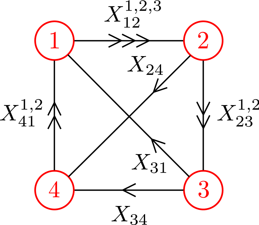
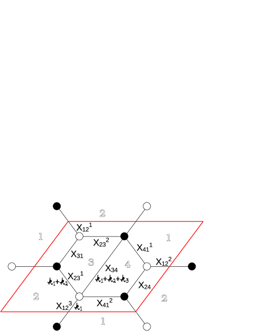
$W=\epsilon^{ab}X_{12}^{a}X_{23}^{b}X_{31}+\epsilon^{ab}X_{41}^{a}X_{12}^{b}X_{24}+\epsilon^{ab}X_{12}^{3}X_{23}^{a}X_{34}X_{41}^{b}$

Figure 16: Quiver diagram, toric diagram, brane tiling (refined by the $n_{ij}$ integers encoding Chern-Simons level) and superpotential of the $dP_{1}$ theory (also called $Y^{2,1}$).

A quiver theory which is a brane tiling theory (under some conditions such that all groups reach an IR conformal fixed point, see e.g. [74]) has a mesonic moduli space which is the symmetric product of $N$ copies of a toric CY₃. An easy way to compute its 2d toric diagram is through the Kasteleyn matrix $K$. Each row of this matrix represents a white node, each column a black node. Each entry is a sum of monomials

$$K_{ab}=\sum_{\gamma\,\in\,\{a\,\rightarrow\,b\}}x^{m_{x}^{(\gamma)}}y^{m_{y}^{(\gamma)}}X_{\gamma}$$ (A.1)

where we sum over the fields $X_{\gamma}$ from the white node $a$ to the black node $b$; then $x,y$ are formal parameters and $m_{x}^{(\gamma)}$, $m_{y}^{(\gamma)}$ are the number of times, with sign, the field $X_{\gamma}$ crosses the $x$ and $y$ boundaries of the fundamental domain. The permanent of $K$ is a sum of terms in $x^{m_{x}}y^{m_{y}}$: each of them represents a point in the 2d toric diagram, with coordinates $(m_{x},m_{y})$. The ambiguity in the choice of fundamental domain translates to $SL(3,\mathbb{Z})$ transformations of the toric diagram. For the $dP_{1}$ example, the Kasteleyn matrix is

$$K=\begin{pmatrix}X_{23}^{2}&X_{31}&X_{12}^{1}\,x^{-1}y\\ X_{34}+X_{12}^{3}\,y^{-1}&X_{23}^{1}&X_{41}^{2}\\ X_{41}^{1}&X_{12}^{2}\,x&X_{24}\end{pmatrix}$$ (A.3)

and its permanent is

$$\operatorname{perm}K=\big{(}X_{12}^{1}X_{12}^{2}X_{12}^{3}+X_{23}^{1}X_{23}^{2}X_{24}+X_{24}X_{31}X_{34}+X_{31}X_{41}^{1}X_{41}^{2}\big{)}\,+\\ +X_{12}^{2}X_{23}^{2}X_{41}^{2}\,x+X_{12}^{3}X_{24}X_{31}\,y^{-1}+X_{12}^{1}X_{12}^{2}X_{34}\,y+X_{12}^{1}X_{23}^{1}X_{41}^{1}\,x^{-1}y\;.$$ (A.4)

The resulting 2d toric diagram (made of 5 points) is in Figure 16.

Each coefficient of a term $x^{m_{x}}y^{m_{y}}$ is in turn a sum of monomials in the fields. Each term is a perfect matching $t_{\rho}$, i.e. a choice of edges in the tiling such that each vertex is touched once and only once. Notice that multiple perfect matchings can lie on the same point in the toric diagram. We write the relations between fields and perfect matchings as:

$$t_{\rho}\,\subset\,\{X_{a}\;|\;a\in R^{-1}(\rho)\}\qquad\quad\leftrightarrow\qquad\quad X_{a}=\prod_{\rho\,\in R(a)}t_{\rho}\;.$$ (A.5)

With a little abuse of notation, $R^{-1}(\rho)$ gives the subset of fields associated to $t_{\rho}$ by $\operatorname{perm}K$, whilst its “inverse” $R(a)$ gives the subset of perfect matchings to which $X_{a}$ is associated. Perfect matchings are useful because they provide a parametrization $X_{a}=\prod_{\rho\,\in R(a)}t_{\rho}$ that automatically solves the F-term equations; they can then be used as fields of a GLSM that reproduces the CY₃ as its moduli space.

An $\mathcal{N}=2$ Chern-Simons quiver gauge theory in 2+1 dimensions is specified by the same data as before, this time considering gauge groups $U(N)_{i}$, plus a collection of CS levels $k_{i}$. Under the condition $\sum_{i}k_{i}=0$, the CS levels can be included in the brane tiling by assigning a number $n_{ij}$ to each chiral field $X_{ij}$:

$$k_{i}=\sum\nolimits_{j}(n_{ij}-n_{ji})\;.$$ (A.6)

This means that each edge contributes $+n_{ij}$ ($-n_{ij}$) to the group on its right (left), looking towards the white node. In Figure 16 we already refined the $dP_{1}$ brane tiling with the integers $n_{ij}$.

A Chern-Simons quiver theory which is a brane tiling has a toric CY₄ geometric moduli space. Its 3d toric diagram can be computed with a refined version of the Kasteleyn matrix algorithm explained above. Each entry $K_{ab}$ is a sum of monomials

$$K_{ab}=\sum_{\gamma\,\in\,\{a\,\rightarrow\,b\}}x^{m_{x}^{(\gamma)}}y^{m_{y}^{(\gamma)}}z^{n^{(\gamma)}}X_{\gamma}$$ (A.7)

where the new formal parameter $z$ is weighted by the number $n_{ij}$ associated with $X_{ij}$. As before, $\operatorname{perm}K$ is a sum of terms $x^{m_{x}}y^{m_{y}}z^{m_{z}}$: each of them represents a point of the 3d toric diagram, of coordinates $(m_{x},m_{y},m_{z})$. The ambiguity in the choice of fundamental domain and of the numbers $n_{ij}$ translates to $SL(4,\mathbb{Z})$ transformations of the toric diagram. For the $dP_{1}$ example, the permanent is

$$\begin{split}\operatorname{perm}K&=X_{31}X_{41}^{1}X_{41}^{2}+X_{12}^{2}X_{23}^{2}X_{41}^{2}\,x+X_{12}^{1}X_{12}^{2}X_{41}^{1}\,x^{-1}y\,+\\ &\quad+X_{12}^{1}X_{12}^{2}X_{12}^{3}\,z^{k_{1}}+X_{12}^{3}X_{24}X_{31}\,y^{-1}z^{k_{1}}+X_{23}^{1}X_{23}^{2}X_{24}\,z^{k_{1}+k_{2}}\,+\\ &\quad+X_{24}X_{31}X_{34}\,z^{k_{1}+k_{2}+k_{3}}+X_{12}^{1}X_{12}^{2}X_{34}\,yz^{k_{1}+k_{2}+k_{3}}\;.\end{split}$$ (A.8)

Notice that setting $z=1$ we reproduce the same algorithm as before. Thus the projection of the 3d toric diagram of the 2+1 dimensional theory on the plane $z=0$ is the 2d toric diagram of the 3+1 dimensional theory.

A.1 Perfect matchings and toric divisors

Each field $X_{ij}$ appears in at least one strictly external perfect matching; when it appears in more than one, the perfect matchings are consecutive along the perimeter of the 2d toric diagram. For fields appearing in a single strictly external perfect matching, the dibaryon is dual to a D3-brane wrapping the radial section of the toric divisor. For fields appearing in more than one perfect matching, the dibaryon is dual to a union of pairwise intersecting D3-branes.

In the $dP_{1}$ example, the perfect matchings and the corresponding points in the toric diagram are

$$a_{0} =\{X_{12}^{2},X_{23}^{2},X_{41}^{2}\}\,=\,(1,0,0)\;, e_{0} =\{X_{12}^{1},X_{12}^{2},X_{12}^{3}\}\,=\,(0,0,0)\;,$$ (A.9)

$$b_{0} =\{X_{12}^{1},X_{12}^{2},X_{34}\}\,=\,(0,1,0)\;, f_{0} =\{X_{23}^{1},X_{23}^{2},X_{24}\}\,=\,(0,0,0)\;,$$

$$c_{0} =\{X_{12}^{1},X_{23}^{1},X_{41}^{1}\}\,=\,(-1,1,0)\;, g_{0} =\{X_{24},X_{31},X_{34}\}\,=\,(0,0,0)\;,$$

$$d_{0} =\{X_{12}^{3},X_{24},X_{31}\}\,=\,(0,-1,0)\;,\qquad h_{0} =\{X_{31},X_{41}^{1},X_{41}^{2}\}\,=\,(0,0,0)\;.$$

The F-term relations of the theory are solved by

$$X_{12}^{1} =b_{0}c_{0}e_{0}\;, X_{41}^{1} =c_{0}h_{0}\;, X_{23}^{1} =c_{0}f_{0}\;, X_{34} =b_{0}g_{0}\;,$$ (A.10)

$$X_{12}^{2} =a_{0}b_{0}e_{0}\;, X_{41}^{2} =a_{0}h_{0}\;, X_{23}^{2} =a_{0}f_{0}\;,$$

$$X_{12}^{3} =d_{0}e_{0}\;, X_{31} =d_{0}g_{0}h_{0}\;, X_{24} =d_{0}f_{0}g_{0}\;.$$

Therefore, some fields represent an irreducible toric divisor: $\{a_{0}=0\}\leftrightarrow\{X_{23}^{2},X_{41}^{2}\}$, $\{b_{0}=0\}\leftrightarrow\{X_{34}\}$, $\{c_{0}=0\}\leftrightarrow\{X_{23}^{1},X_{41}^{1}\}$, $\{d_{0}=0\}\leftrightarrow\{X_{12}^{3},X_{24},X_{31}\}$; other fields represent a collection of pairwise intersecting toric divisors: $\{a_{0}b_{0}=0\}\leftrightarrow\{X_{12}^{2}\}$, $\{b_{0}c_{0}=0\}\leftrightarrow\{X_{12}^{1}\}$.

Appendix B Moduli space of flavored quivers and the A-theory

In this appendix we prove that the geometric moduli space of the A-theory is the same as $\mathcal{M}_{\mathrm{flav}}$ in (4.20).

Consider a single bifundamental $X_{\alpha}\equiv X_{ij}$ flavored by $h_{\alpha}$ quarks $(p_{\alpha},q_{\alpha})$ in the flavored theory. In the A-theory $X_{ij}$ has been substituted by $h_{\alpha}+1$ bifundamentals $C_{i1}$, $C_{12}$, …, $C_{h_{\alpha}j}$, $h_{\alpha}$ new gauge groups $U(1)^{(l)}_{1}$ with $l=1,\dots,h_{\alpha}$ have been added, and the other two gauge groups involved have CS levels $k_{i}-\gamma_{\alpha}$ and $k_{j}+\gamma_{\alpha}-h_{\alpha}$, with $0\leq\gamma_{\alpha}\leq h_{\alpha}$, in terms of the levels $k_{i}$ and $k_{j}$ before flavoring. As we showed in Section 4.1, the geometric moduli space of the A-theory is the Kähler quotient

$$\mathcal{M}_{\mathrm{A-theory}}=\{X_{a},R,\tilde{R}\;|\;dW_{A}=0,\;R\tilde{R}=1\}//U(1)^{\tilde{G}}\;,$$ (B.1)

where $R,\tilde{R}$ are the monopoles in the A-theory, $W_{A}$ its superpotential and $\tilde{G}=G+h_{\alpha}$ is the total number of gauge groups.

The only fields charged under the $h_{\alpha}$ new groups $U(1)^{(l)}_{1}$ are $C_{i1},C_{12},\dots,C_{h_{\alpha}j}$, $R$ and $\tilde{R}$. Their charges, including $U(1)_{k_{i}-\gamma_{\alpha}}$ and $U(1)_{k_{j}+\gamma_{\alpha}-h_{\alpha}}$, are:

$$\begin{array}[]{c|ccccccc}&C_{i1}&C_{12}&\dots&C_{h_{\alpha}-1,h_{\alpha}}&C_{h_{\alpha}j}&R&\tilde{R}\\ \hline\cr\rule[-5.16663pt]{0.0pt}{16.79158pt}U(1)_{k_{i}-\gamma_{\alpha}}&1&0&\dots&0&0&k_{i}-\gamma_{\alpha}&-k_{i}+\gamma_{\alpha}\\ \rule[-5.16663pt]{0.0pt}{16.79158pt}U(1)^{(1)}_{1}&-1&1&&0&0&1&-1\\ \rule[-5.16663pt]{0.0pt}{16.79158pt}U(1)^{(2)}_{1}&0&-1&&0&0&1&-1\\ \vdots&\vdots&\vdots&&\vdots&\vdots&\vdots&\vdots\\ U(1)^{(h_{\alpha}-1)}_{1}&0&0&&1&0&1&-1\\ U(1)^{(h_{\alpha})}_{1}&0&0&&-1&1&1&-1\\ U(1)_{k_{j}+\gamma_{\alpha}-h_{\alpha}}&0&0&\dots&0&-1&\;\;k_{j}+\gamma_{\alpha}-h_{\alpha}&-k_{j}-\gamma_{\alpha}+h_{\alpha}\end{array}$$

Let us perform the Kähler quotient by the complexified gauge group $\prod_{l=1}^{h_{\alpha}}U(1)^{(l)}_{1}$ only: it is done by introducing gauge invariants and relations between them. The independent gauge invariants are:

$$T \equiv R\,(C_{i1})^{h_{\alpha}}(C_{12})^{h_{\alpha}-1}\dots(C_{h_{\alpha}-1,h_{\alpha}})^{1}\qquad\qquad R\tilde{R} =1$$ (B.2)

$$\tilde{T} \equiv\tilde{R}\,(C_{12})^{1}(C_{23})^{2}\dots(C_{h_{\alpha}j})^{h_{\alpha}} X_{ij} \equiv C_{i1}C_{12}\dots C_{h_{\alpha}j}\;,$$

where we dubbed one of them as the old field $X_{ij}$. The only relation is

$$T\tilde{T}=(X_{ij})^{h_{\alpha}}\;.$$ (B.3)

We see that, after quotienting, the new monopole operators are $T$, $\tilde{T}$ and obey a “quantum” F-term relation. The charges of $X_{ij}$, $T$, $\tilde{T}$ under the remaining two groups are:

$$\begin{array}[]{c|ccc}&X_{ij}&T&\tilde{T}\\ \hline\cr\rule[-5.16663pt]{0.0pt}{16.79158pt}U(1)_{k_{i}-\gamma_{\alpha}}&1&\;\;k_{i}-\gamma_{\alpha}+h_{\alpha}&-k_{i}+\gamma_{\alpha}\\ \rule[-5.16663pt]{0.0pt}{16.79158pt}U(1)_{k_{j}+\gamma_{\alpha}-h_{\alpha}}&-1&k_{j}+\gamma_{\alpha}-h_{\alpha}&-k_{j}-\gamma_{\alpha}\end{array}$$

We want to compare these charges with those in the flavored theory. When the flavored theory is being flavored by $h_{\alpha}$ quarks, its CS levels have to be shifted by $\delta k_{l}=\big{(}\frac{h_{\alpha}}{2}-\gamma_{\alpha}\big{)}\,g_{l}[X_{ij}]$ (3.4), where $\gamma_{\alpha}$ is a choice of theory. Plugging into (3.13) we get:

$$g_{l}[T]=k_{l}+(h_{\alpha}-\gamma_{\alpha})\,g_{l}[X_{ij}]\qquad\qquad g_{l}[\tilde{T}]=-k_{l}+\gamma_{\alpha}\,g_{l}[X_{ij}]\;.$$ (B.4)

This precisely agrees with the table above if we identify the choice of $0\leq\gamma_{\alpha}\leq h_{\alpha}$ between the flavored and A-theory. So the quotient by $\prod_{l=1}^{h_{\alpha}}U(1)^{(l)}_{1}$ gives the A-theory monopoles the same quantum charges as in the flavored theory.

Let us now consider the classical F-term relations. In the A-theory, the F-terms are of two sorts: differentiating $W_{A}$ by a field which is not $C_{i1},\dots,C_{h_{\alpha}j}$ we get the same equation as in the flavored theory, but with $X_{ij}\to C_{i1}\dots C_{h_{\alpha}j}$; differentiating $W_{A}$ by one of $C_{i1},\dots,C_{h_{\alpha}j}$ we get the same equation as in the flavored theory, but multiplied by the other $C$ fields:

$$\big{(}\prod C\big{)}\,(\text{flavored theory relation})=0\;.$$ (B.5)

As long as no more than one of the $C$ fields vanishes, we exactly reproduce the same F-terms as in the flavored theory. When more than one $C$ field vanishes, all equations become trivial and the A-theory could develop a branch which is not contained in the geometric moduli space of the flavored theory. However, the geometric moduli space of the A-theory (which is the CY₄) is the one where the F-terms are solved by the parametrization $X_{a}=\prod_{\rho\,\in R(a)}t_{\rho}$ (4.16), thus if the flavored theory relations are satisfied at $C\neq 0$, they are satisfied also at $C=0$.

We have thus shown that:

$$\begin{split}\mathcal{M}_{\mathrm{A-theory}}&=\{X_{a}^{A}\;|\;dW_{A}=0\}//U(1)^{\tilde{G}-2}=\\ &=\{X_{a}^{A},R,\tilde{R}\;|\;dW_{A}=0,\;R\tilde{R}=1\}//U(1)^{\tilde{G}}=\\ &=\{X_{a}^{F},T,\tilde{T}\;|\;dW_{F}=0,\;T\tilde{T}=\prod X_{\alpha}^{h_{\alpha}}\}//U(1)^{G}=\mathcal{M}_{\mathrm{flav}}\;.\end{split}$$ (B.6)

The argument is straightforwardly generalized to the case that we flavor multiple fields $X_{\alpha}$, each with its own $h_{\alpha}$ quarks. This concludes the proof.

Let us conclude with a remark. Suppose that the theory before flavoring has some global Abelian symmetry, under which $X_{ij}$ has charge $Q$. Then also the A-theory has such a symmetry, if we assign charges $Q/(h_{\alpha}+1)$ to $C_{i1},\dots,C_{h_{\alpha}j}$. It is easy to compute that, after modding out by $\prod_{l}U(1)^{(l)}_{1}$, both $T$ and $\tilde{T}$ have charge $h_{\alpha}Q/2$. This reproduces the quantum formulæ (3.12) and (3.14).

References

- [1] O. Aharony, O. Bergman, D. L. Jafferis, and J. Maldacena, “N=6 superconformal Chern-Simons-matter theories, M2-branes and their gravity duals,” JHEP 10 (2008) 091, arXiv:0806.1218 [hep-th].
- [2] M. Benna, I. Klebanov, T. Klose, and M. Smedback, “Superconformal Chern-Simons Theories and AdS4/CFT3 Correspondence,” JHEP 09 (2008) 072, arXiv:0806.1519 [hep-th].
- [3] Y. Imamura and K. Kimura, “On the moduli space of elliptic Maxwell-Chern-Simons theories,” Prog. Theor. Phys. 120 (2008) 509–523, arXiv:0806.3727 [hep-th].
- [4] K. Hosomichi, K.-M. Lee, S. Lee, S. Lee, and J. Park, “N=5,6 Superconformal Chern-Simons Theories and M2-branes on Orbifolds,” JHEP 09 (2008) 002, arXiv:0806.4977 [hep-th].
- [5] O. Aharony, O. Bergman, and D. L. Jafferis, “Fractional M2-branes,” JHEP 11 (2008) 043, arXiv:0807.4924 [hep-th].
- [6] D. L. Jafferis and A. Tomasiello, “A simple class of N=3 gauge/gravity duals,” JHEP 10 (2008) 101, arXiv:0808.0864 [hep-th].
- [7] D. Martelli and J. Sparks, “Moduli spaces of Chern-Simons quiver gauge theories and AdS(4)/CFT(3),” Phys. Rev. D78 (2008) 126005, arXiv:0808.0912 [hep-th].
- [8] A. Hanany and A. Zaffaroni, “Tilings, Chern-Simons Theories and M2 Branes,” JHEP 10 (2008) 111, arXiv:0808.1244 [hep-th].
- [9] K. Ueda and M. Yamazaki, “Toric Calabi-Yau four-folds dual to Chern-Simons-matter theories,” JHEP 12 (2008) 045, arXiv:0808.3768 [hep-th].
- [10] Y. Imamura and K. Kimura, “Quiver Chern-Simons theories and crystals,” JHEP 10 (2008) 114, arXiv:0808.4155 [hep-th].
- [11] A. Hanany, D. Vegh, and A. Zaffaroni, “Brane Tilings and M2 Branes,” JHEP 03 (2009) 012, arXiv:0809.1440 [hep-th].
- [12] S. Franco, A. Hanany, J. Park, and D. Rodriguez-Gomez, “Towards M2-brane Theories for Generic Toric Singularities,” JHEP 12 (2008) 110, arXiv:0809.3237 [hep-th].
- [13] A. Hanany and Y.-H. He, “M2-Branes and Quiver Chern-Simons: A Taxonomic Study,” arXiv:0811.4044 [hep-th].
- [14] A. Amariti, D. Forcella, L. Girardello, and A. Mariotti, “3D Seiberg-like Dualities and M2 Branes,” arXiv:0903.3222 [hep-th].
- [15] S. Franco, I. R. Klebanov, and D. Rodriguez-Gomez, “M2-branes on Orbifolds of the Cone over ,” JHEP 08 (2009) 033, arXiv:0903.3231 [hep-th].
- [16] J. Davey, A. Hanany, N. Mekareeya, and G. Torri, “Phases of M2-brane Theories,” JHEP 06 (2009) 025, arXiv:0903.3234 [hep-th].
- [17] M. Aganagic, “A Stringy Origin of M2 Brane Chern-Simons Theories,” arXiv:0905.3415 [hep-th].
- [18] J. Davey, A. Hanany, N. Mekareeya, and G. Torri, “Higgsing M2-brane Theories,” JHEP 11 (2009) 028, arXiv:0908.4033 [hep-th].
- [19] D. Martelli and J. Sparks, “AdS4/CFT3 duals from M2-branes at hypersurface singularities and their deformations,” arXiv:0909.2036 [hep-th].
- [20] J. Davey, A. Hanany, and J. Pasukonis, “On the Classification of Brane Tilings,” arXiv:0909.2868 [hep-th].
- [21] J. Hewlett and Y.-H. He, “Probing the Space of Toric Quiver Theories,” arXiv:0909.2879 [hep-th].
- [22] M. Taki, “M2-branes Theories without 3+1 Dimensional Parents via Un- Higgsing,” arXiv:0910.0370 [hep-th].
- [23] H. Ooguri and C.-S. Park, “Superconformal Chern-Simons Theories and the Squashed Seven Sphere,” JHEP 11 (2008) 082, arXiv:0808.0500 [hep-th].
- [24] D. Gaiotto and A. Tomasiello, “The gauge dual of Romans mass,” arXiv:0901.0969 [hep-th].
- [25] N. Bobev, N. Halmagyi, K. Pilch, and N. P. Warner, “Holographic, N=1 Supersymmetric RG Flows on M2 Branes,” JHEP 09 (2009) 043, arXiv:0901.2736 [hep-th].
- [26] D. Forcella and A. Zaffaroni, “N=1 Chern-Simons theories, orientifolds and Spin(7) cones,” arXiv:0911.2595 [hep-th].
- [27] D. Gaiotto and D. L. Jafferis, “Notes on adding D6 branes wrapping RP3 in AdS4 x CP3,” arXiv:0903.2175 [hep-th].
- [28] S. Hohenegger and I. Kirsch, “A note on the holography of Chern-Simons matter theories with flavour,” JHEP 04 (2009) 129, arXiv:0903.1730 [hep-th].
- [29] Y. Hikida, W. Li, and T. Takayanagi, “ABJM with Flavors and FQHE,” JHEP 07 (2009) 065, arXiv:0903.2194 [hep-th].
- [30] M. Fujita and T.-S. Tai, “Eschenburg space as gravity dual of flavored N=4 Chern- Simons-matter theory,” JHEP 09 (2009) 062, arXiv:0906.0253 [hep-th].
- [31] K. Jensen and A. Karch, “ABJM Mirrors and a Duality of Dualities,” JHEP 09 (2009) 004, arXiv:0906.3013 [hep-th].
- [32] M. Ammon, J. Erdmenger, R. Meyer, A. O’Bannon, and T. Wrase, “Adding Flavor to AdS4/CFT3,” arXiv:0909.3845 [hep-th].
- [33] D. L. Jafferis, I. R. Klebanov, and S. S. Pufu. Work in progress.
- [34] G. ’t Hooft, “On the Phase Transition Towards Permanent Quark Confinement,” Nucl. Phys. B138 (1978) 1.
- [35] A. M. Polyakov, “Quark Confinement and Topology of Gauge Groups,” Nucl. Phys. B120 (1977) 429–458.
- [36] G. W. Moore and N. Seiberg, “Taming the Conformal Zoo,” Phys. Lett. B220 (1989) 422.
- [37] V. Borokhov, A. Kapustin, and X.-k. Wu, “Topological disorder operators in three-dimensional conformal field theory,” JHEP 11 (2002) 049, arXiv:hep-th/0206054.
- [38] V. Borokhov, A. Kapustin, and X.-k. Wu, “Monopole operators and mirror symmetry in three dimensions,” JHEP 12 (2002) 044, arXiv:hep-th/0207074.
- [39] V. Borokhov, “Monopole operators in three-dimensional N = 4 SYM and mirror symmetry,” JHEP 03 (2004) 008, arXiv:hep-th/0310254.
- [40] N. Itzhaki, “Anyons, ’t Hooft loops and a generalized connection in three dimensions,” Phys. Rev. D67 (2003) 065008, arXiv:hep-th/0211140.
- [41] M. K. Benna, I. R. Klebanov, and T. Klose, “Charges of Monopole Operators in Chern-Simons Yang-Mills Theory,” arXiv:0906.3008 [hep-th].
- [42] D. L. Jafferis, “M2-branes, CS theories and AdS4/CFT3,”. Talk given at Strings 2009, Roma June 22-26, 2009, http://strings2009.roma2.infn.it/talks/Jafferis_Strings09.pdf.
- [43] D. L. Jafferis, “Quantum corrections to N=2 Chern-Simons theories with flavor and their AdS4 duals,” arXiv:0911.4324 [hep-th].
- [44] S. Franco, A. Hanany, D. Martelli, J. Sparks, D. Vegh, and B. Wecht, “Gauge theories from toric geometry and brane tilings,” JHEP 01 (2006) 128, arXiv:hep-th/0505211.
- [45] K. D. Kennaway, “Brane Tilings,” Int. J. Mod. Phys. A22 (2007) 2977–3038, arXiv:0706.1660 [hep-th].
- [46] M. Yamazaki, “Brane Tilings and Their Applications,” Fortsch. Phys. 56 (2008) 555–686, arXiv:0803.4474 [hep-th].
- [47] C. Closset, “Toric geometry and local Calabi-Yau varieties: An introduction to toric geometry (for physicists),” arXiv:0901.3695 [hep-th].
- [48] A. Hanany and D. Vegh, “Quivers, tilings, branes and rhombi,” JHEP 10 (2007) 029, arXiv:hep-th/0511063.
- [49] B. Feng, Y.-H. He, K. D. Kennaway, and C. Vafa, “Dimer models from mirror symmetry and quivering amoebae,” Adv. Theor. Math. Phys. 12 (2008) 3, arXiv:hep-th/0511287.
- [50] A. Hanany and A. Iqbal, “Quiver theories from D6-branes via mirror symmetry,” JHEP 04 (2002) 009, arXiv:hep-th/0108137.
- [51] D. Berenstein, C. P. Herzog, and I. R. Klebanov, “Baryon spectra and AdS/CFT correspondence,” JHEP 06 (2002) 047, arXiv:hep-th/0202150.
- [52] A. Butti, D. Forcella, and A. Zaffaroni, “Counting BPS baryonic operators in CFTs with Sasaki- Einstein duals,” JHEP 06 (2007) 069, arXiv:hep-th/0611229.
- [53] P. W. Kasteleyn, “Graph theory and crystal physics,” Graph theory and theoretical physics 43–110. Academic Press, London, 1967.
- [54] A. Hanany and K. D. Kennaway, “Dimer models and toric diagrams,” arXiv:hep-th/0503149.
- [55] S. Franco, A. Hanany, K. D. Kennaway, D. Vegh, and B. Wecht, “Brane Dimers and Quiver Gauge Theories,” JHEP 01 (2006) 096, arXiv:hep-th/0504110.
- [56] P. Ouyang, “Holomorphic D7-branes and flavored gauge theories,” Nucl. Phys. B699 (2004) 207–225, arXiv:hep-th/0311084.
- [57] S. Franco and A. M. . Uranga, “Dynamical SUSY breaking at meta-stable minima from D- branes at obstructed geometries,” JHEP 06 (2006) 031, arXiv:hep-th/0604136.
- [58] F. Benini, F. Canoura, S. Cremonesi, C. Nunez, and A. V. Ramallo, “Unquenched flavors in the Klebanov-Witten model,” JHEP 02 (2007) 090, arXiv:hep-th/0612118.
- [59] F. Benini, F. Canoura, S. Cremonesi, C. Nunez, and A. V. Ramallo, “Backreacting Flavors in the Klebanov-Strassler Background,” JHEP 09 (2007) 109, arXiv:0706.1238 [hep-th].
- [60] F. Benini, “A chiral cascade via backreacting D7-branes with flux,” JHEP 10 (2008) 051, arXiv:0710.0374 [hep-th].
- [61] A. J. Niemi and G. W. Semenoff, “Axial Anomaly Induced Fermion Fractionization and Effective Gauge Theory Actions in Odd Dimensional Space- Times,” Phys. Rev. Lett. 51 (1983) 2077.
- [62] A. N. Redlich, “Gauge Noninvariance and Parity Nonconservation of Three-Dimensional Fermions,” Phys. Rev. Lett. 52 (1984) 18.
- [63] A. N. Redlich, “Parity Violation and Gauge Noninvariance of the Effective Gauge Field Action in Three-Dimensions,” Phys. Rev. D29 (1984) 2366–2374.
- [64] S. A. Cherkis and A. Hashimoto, “Supergravity solution of intersecting branes and AdS/CFT with flavor,” JHEP 11 (2002) 036, arXiv:hep-th/0210105.
- [65] M. S. Bianchi, S. Penati, and M. Siani, “Infrared stability of ABJ-like theories,” arXiv:0910.5200 [hep-th].
- [66] J. de Boer, K. Hori, and Y. Oz, “Dynamics of N = 2 supersymmetric gauge theories in three dimensions,” Nucl. Phys. B500 (1997) 163–191, arXiv:hep-th/9703100.
- [67] O. Aharony, A. Hanany, K. A. Intriligator, N. Seiberg, and M. J. Strassler, “Aspects of N = 2 supersymmetric gauge theories in three dimensions,” Nucl. Phys. B499 (1997) 67–99, arXiv:hep-th/9703110.
- [68] J. Choi, S. Lee, and J. Song, “Superconformal Indices for Orbifold Chern-Simons Theories,” JHEP 03 (2009) 099, arXiv:0811.2855 [hep-th].
- [69] D. Rodriguez-Gomez, “M5 spikes and operators in the HVZ membrane theory,” arXiv:0911.0008 [hep-th].
- [70] D. Martelli and J. Sparks, “Notes on toric Sasaki-Einstein seven-manifolds and ,” JHEP 11 (2008) 016, arXiv:0808.0904 [hep-th].
- [71] N. Benishti, Y.-H. He, and J. Sparks, “(Un)Higgsing the M2-brane,” arXiv:0909.4557 [hep-th].
- [72] D. Gaiotto and A. Tomasiello, “Perturbing gauge/gravity duals by a Romans mass,” arXiv:0904.3959 [hep-th].
- [73] B. S. Acharya, F. Benini, and R. Valandro, “Fixing moduli in exact type IIA flux vacua,” JHEP 02 (2007) 018, arXiv:hep-th/0607223.
- [74] D. R. Gulotta, “Properly ordered dimers, -charges, and an efficient inverse algorithm,” JHEP 10 (2008) 014, arXiv:0807.3012 [hep-th].